A nc-AFM simulator with Phase Locked Loop-controlled frequency detection and excitation

Abstract

A simulation of an atomic force microscope operating in the constant amplitude dynamic mode is described. The implementation mimics the electronics of a real setup which includes a digital Phase Locked Loop (PLL). The PLL is not only used as a very sensitive frequency detector, but also to generate the time-dependent phase-shifted signal which drives the cantilever. The optimum adjustments of individual functional blocks and their joint performance in typical experiments are determined in details. Prior to testing the complete setup, the performances of the numerical PLL and of the amplitude controller were ascertained to be satisfactory compared to those of the real components. Attention is also focussed on the issue of apparent dissipation, that is of spurious variations in the driving amplitude caused by the non-linear interaction occurring between the tip and the surface and by the finite response times of the various controllers. To do so, an estimate of the minimum dissipated energy which is detectable by the instrument upon operating conditions is given. This allows to discuss the relevance of apparent dissipation which can be conditionally generated with the simulator in comparison to values reported experimentally. The analysis emphasizes that apparent dissipation can contribute to the measured dissipation up to $15\%$ of the intrinsic dissipated energy of the cantilever, but can be made negligible when properly adjusting the controllers, the PLL gains and the scan speed. It is inferred that the experimental values of dissipation reported cannot only originate in apparent dissipation, which favors the hypothesis of “physical” channels of dissipation.

I Introduction

Since almost a decade, non-contact atomic force microscopy (nc-AFM) has proven capable of yielding images showing contrasts down to atomic scale on metals, semiconductors, as well as insulating ionic crystals, with or without metallic or adsorbate overlayers morita02a ; garcia02a ; giessibl03a . Like other scanning force methods, the technique relies on a micro-fabricated tip grown at the end of a cantilever. However, unlike the widely used contact or the tapping modes, the cantilever deflection is neither static nor driven at constant frequency, but is driven at a frequency $\widetilde{f_{0}}=\widetilde{\omega_{0}}/2\pi$ equal to its fundamental bending resonance frequency, slightly shifted by the tip-sample interaction. A sufficiently large oscillation amplitude prevents snap into contact. A quality factor exceeding $10^{4}$, readily achieved in UHV, together with frequency detection by demodulation provide unprecedented force sensitivity albrecht91a ; duerig92a . A phase-locked loop (PLL) is typically used for that purpose. Since $\widetilde{f_{0}}$ varies with the tip-surface distance, it deviates from $f_{0}$, the fundamental bending eigenfrequency of the free cantilever. Upon approaching the surface, the tip is first attracted, in particular by Van der Waals forces, which decrease $\widetilde{f_{0}}$. The negative frequency shift, $\Delta f=\widetilde{f_{0}}-f_{0}$, varies rapidly with the minimum tip-distance $d$, usually as $d^{-n}$ with $n\geq 1.5$, and then as $\exp(-d/\lambda)$ a few angströms above the surface, owing to short-range chemical and/or steric forces guggisberg00a . When $\Delta f$ is used for distance control, contrasts down to the atomic scale can be achieved. Another specific feature of the nc-AFM technique is that the oscillation amplitude $A$ is kept constant while approaching or scanning the surface at constant $\Delta f$.

Controlling the phase of the excitation so as to maintain it on resonance and to make the frequency matching a preset $\widetilde{f_{0}}$-value, as well as the driving amplitude so as to keep the tip oscillation amplitude constant, respectively, requires dedicated electronic components. Amplitude control is usually achieved using a proportional integral controller (PIC), hereafter referred to as APIC, whereas phase and frequency control can be performed in two ways. In both cases the AC deflection signal of the cantilever is filtered, then phase-shifted and multiplied by the APIC output and by a suitable gain. The most common method consists in using a band-pass filtered deflection signal gauthier02a ; couturier03a . This is referred to as the self-excitation mode. The second method, extensively analyzed hereafter, consists in using the PLL to generate the time-dependent phase of the excitation signal. The PLL output is driven by the AC deflection signal and phase-locked to it, provided that the PLL settings are properly adjusted. Then, the PLL continuously tracks the oscillator frequency $\widetilde{f_{0}}$ with high precision. Moreover, the phase lag introduced by the PLL itself can be compensated. For reasons of clarity, this mode will be referred to as the PLL-excitation mode. The choice of the PLL as the excitation source has initially been motivated to take benefit of the noise reduction due to PLLs BEST . A further advantage is that the noise reduction does not only optimize the detection of the frequency shift, but also the excitation signal. In both modes, the phase shifter is adjusted so as the phase lag $\varphi$ between the excitation and the tip oscillation equals $-\pi/2$ rad throughout an experiment. If all adjustments and controls were perfect, the oscillator would then always remain on resonance.

The nc-AFM technique therefore requires the simultaneous operation of three controllers : PLL, APIC and distance controller, which keeps constant a given $\Delta f$ while scanning the surface. Since the tip-surface interaction makes the dynamic of the oscillator non-linear, the combined action of those three controllers becomes complex. They can conditionally interplay gauthier02a ; couturier03a and therefore influence the dynamics of the system. Consider for instance the time the PLL spends to track $\widetilde{f_{0}}$ is long compared to the time constant of the APIC. Then, the cantilever is no longer maintained at $\widetilde{f_{0}}$, but at a frequency slightly higher or lower. Consequently, the oscillation amplitude drops note_virtual11 and the APIC increases the excitation to correct the amplitude reduction. Such an apparent loss of energy, which can as well be interpreted as a damping increase of the cantilever, does not result of a dissipative process occurring between the tip and the surface, but is the consequence of the bad tracking of $\widetilde{f_{0}}$. So-called apparent dissipation (or apparent damping) remains under discussions in the nc-AFM community, which hinders the quantitative interpretation of the experimental proofs of dissipative phenomena on the atomic scale over a wide variety of samples gotsmann99a ; loppacher00a ; loppacher00b ; bennewitz00a ; gotsmann01a ; hoffmann01b ; giessibl02b ; hoffmann03a ; pfeiffer04a ; hembacher05a . Thus, addressing the problem of apparent dissipation turns out to be mandatory but requires to understand the complex interplay between controllers as well as to analyze the system time constants. Although several models of physical dissipation, connected or not to the conservative tip-surface interaction have been proposed gauthier99a ; sasaki00a ; gauthier00a ; duerig00b ; kantorovich01b ; boisgard02a ; boisgard02b ; trevethan04a ; trevethan04b ; kantorovich04a and reviewed note_virtual08 , the question of apparent dissipation in the self-excitation scheme has been addressed by two groups gauthier02a ; couturier02a ; couturier03a . M. Gauthier et al. [gauthier02a, ] emphasize the interplay between the controllers and the conservative tip-sample interaction which, although weak, can significantly affect the damping. They put in evidence resonance effects which can conditionally occur in damping images upon scan speed and APIC gains. G. Couturier et al. couturier03a address a similar problem numerically and analytically. They show that the self-excited oscillator can be conditionally stable within a narrow domain of $K_{p}$ and $K_{i}$ gains of the APIC, but that consequent damping variations can as well be generated upon conservative force steps which change the borders of the stability domain. The results mentioned above are valid for the self-excitation mode, but the question of apparent dissipation remains open regarding the PLL-excitation mode. However recently, J. Polesel-Maris and S. Gauthier [polesel05, ] have proposed a virtual dynamic AFM based on the PLL-excitation scheme. Their work is targeted at images calculations including realistic force fields obtained from molecular dynamics calculations note_virtual12 . Their conclusions stress the contribution of the scanning speed and of the experimental noise to images distortion but do not address the potential contribution of the PLL upon operating conditions.

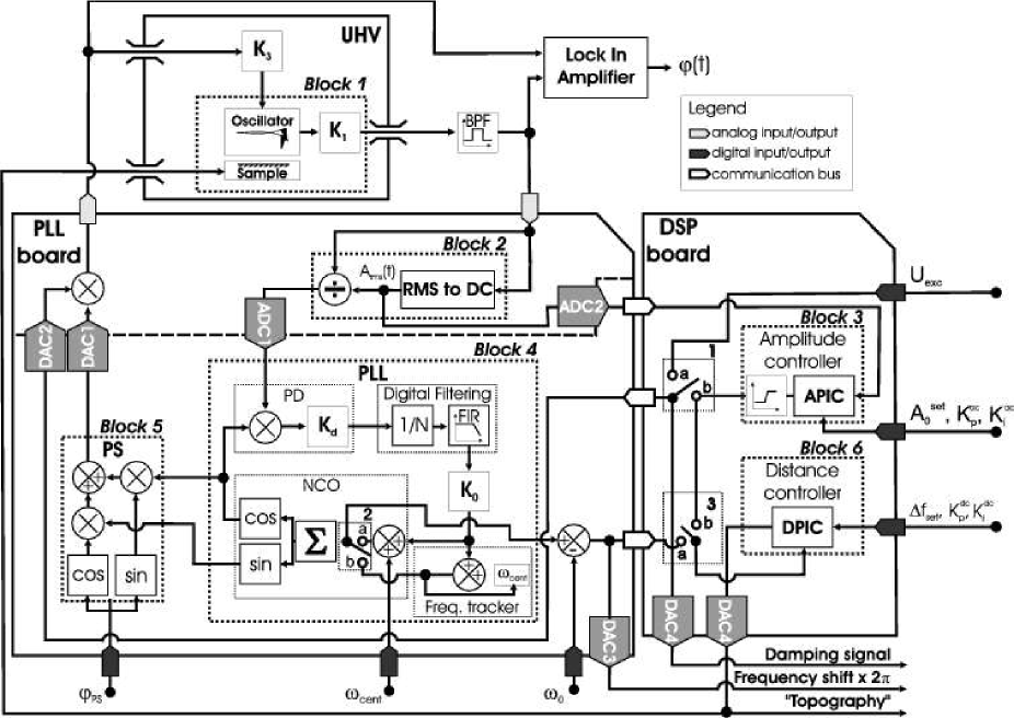
Figure 1: Scheme of the simulator operating in nc-AFM, based on the design of the electronics of the real apparatus.

The goal of the present work is two-fold : 1- providing a detailed description of the PLL-excitation based electronics of a home-built AFM used in our laboratory; 2- assessing the contribution of the various controllers to the dissipation signal and in particular the contribution of the PLL. The paper is organized as follows. In section II, an overview of the chart of the microscope and of the attached electronics (cf. fig.1), is given in terms of blocks, namely ; oscillator and optical detection (block 1), RMS-to-DC converter (block 2), amplitude controller (block 3), PLL (block 4), phase shifter (block 5) and tip-surface distance controller (block 6). In section III, the detailed description of the numerical scheme used to perform the calculations is given on the base of coupled integro-differential equations ruling each block. Section IV provides an estimate of the minimum detectable dissipation by the instrument with the goal to assess the relevance, compared to experimental results, of the apparent dissipation which can be conditionally generated numerically. Section V reports the results. In the first part, the simulation is validated by comparing a numerical $\Delta f$ vs. distance curve to the analytic expression of the $\Delta f$ due to Morse and Van der Waals interactions which does not take into account the finite response of the various controllers. Then the dynamic properties of the numerical PLL and APIC upon gains are compared to those of the real components. Section V.3 gives some examples on how apparent dissipation can be produced upon working conditions of the PLL. Section V.4 finally shows scan lines computed while varying PLL gains, scan speed and APIC gains. A discussion and a conclusion end the article.

II Overview

II.1 Description

The electronics consists of analog and digital ($12$ bits) circuits which are described by six interconnected main blocks operating at various sampling frequencies ($f_{s}$). The highest sampling frequency among the digital blocks is the PLL one, $f_{s_{1}}=20$ MHz. The PLL electronics has initially been developped by Ch.Loppacher [loppacher98a, ].

Block $1$ represents the detected oscillating tip motion coupled to the sample surface. In the simulation, the block is described by an equivalent analog circuit. More generally, all the analog parts of the electronics are described in the simulation using a larger sampling frequency compared to $f_{s_{1}}$, namely $f_{s_{2}}=400$ MHz. This is motivated by the ultra-high vacuum environment within which the microscope is placed, thus resulting in a high quality factor of the cantilever, typically $Q=30000$ at room temperature. Besides, nc-AFM cantilevers have typical fundamental eigenfrequencies $f_{0}\simeq 150$ kHz. The chosen sampling frequency should therefore insure a proper integration of the differential equations with an error weak enough. The signal of the oscillating cantilever motion goes into a band pass filter which cuts-off its low and high frequencies components. The bandwidth of the filter is typically $60$ kHz, centered on the resonance frequency of the cantilever. Despite the filter has been implemented in the simulation, no noise has been considered, so far. The signal is then sent to other blocks depicting the interconnected parts of two boards, namely an analog/digital one, the “PLL board”, and a fully digital one which integrates a Digital Signal Processor (DSP), the “DSP board”. The boards share data via a “communication bus” operating at $f_{s_{3}}=10$ kHz, the lowest frequency of the digital electronics.

Block $2$ stands for the lone analog part of the PLL board ($f_{s}=f_{s_{2}}$). It consists of a RMS-to-DC converter. The block output is the rms value of the oscillations amplitude, $A_{\text{rms}}(t)$. $A_{\text{rms}}(t)$ is provided to block 3, one of the two PICs implemented on the DSP ($f_{s}=f_{s_{3}}$). When operating in the nc-AFM mode, the block output is the DC value of the driving amplitude which maintains constant the reference value of the oscillations amplitude, $A_{0}^{\text{set}}$. This is why it is referred to as the amplitude controller, APIC. For technical reasons due to the chips, the signal is saturated between $0$ and $10$ V.

The dashed line in fig.1 depicts the border between analog and digital circuits in the PLL board. The digital PLL, block $4$ ($f_{s}=f_{s_{1}}$), consists of three sub-blocks : a Phase Detector (PD), a Numerical Controlled Oscillator (NCO) and a filtering stage consisting of a decimation filter and a Finite Impulse Response (FIR) low pass filter in series. The PLL receives the signal of the oscillation divided by $A_{\text{rms}}(t)$ plus an external parameter : the “center frequency”, $f_{\text{cent}}=\omega_{\text{cent}}/2\pi$. $f_{\text{cent}}$ specifies the frequency to which the input signal has to be compared to for the demodulation frequency stage. This point is particularly addressed in section III.4. The NCO generates the digital $\sin$ and $\cos$ waveforms of the time-dependent phase, $\varphi_{\text{nco}}(t)+\varphi_{\text{pll}}$(t), ideally identical to the one of the input signal. $\varphi_{\text{pll}}(t)$ is correlated to the error which is potentially produced while the frequency demodulation, upon operating conditions. The $\sin$ and $\cos$ waveforms are then sent to a digital phase shifter, block $5$ ($f_{s}=f_{s_{1}}$) which shifts the incoming phase $\varphi_{\text{nco}}(t)+\varphi_{\text{pll}}(t)$ by a constant amount, $\varphi_{\text{ps}}$, set by the user. Since the cantilever is usually driven at $\widetilde{f_{0}}$, $\varphi_{\text{ps}}$ is adjusted to make that condition fulfilled note_virtual13 , namely :

$$\varphi_{\text{nco}}(t)+\varphi_{\text{pll}}(t)+\varphi_{\text{ps}}=\widetilde{\omega_{0}}t,$$ (1)

Indeed, the PLL produces the phase locked to the input, that is $\varphi_{\text{nco}}(t)+\varphi_{\text{pll}}(t)\simeq\widetilde{\omega_{0}}t-\pi/2$. If it optimally operates, $\varphi_{\text{pll}}(t)\simeq 0$. $\varphi_{\text{ps}}$ has therefore to be set equal to $+\pi/2$ to maintain the excitation at the resonance frequency prior to starting the experiments. Consequently, $\varphi=-\pi/2$ rad. The block output, $\sin\left[\varphi_{\text{nco}}(t)+\varphi_{\text{pll}}(t)+\varphi_{\text{ps}}\right]$, is converted into an analog signal and then multiplied by the APIC output, thus generating the full AC excitation applied to the piezoelectric actuator to drive the cantilever.

Block $6$ is the second PIC of the DSP ($f_{s}=f_{s_{3}}$). It controls the tip-surface distance to maintain constant either a given value of the frequency shift, or a given value of the driving amplitude while performing a scan line (switch $3$ set to location “a” or “b”, respectively in fig.1). The output is the so-called “topography” signal. The block is referred to as the distance controller, DPIC.

Finally, a digital lock-in amplifier detects the phase lag, $\varphi$, between the excitation signal provided to the oscillator and the oscillating cantilever motion.

II.2 Time considerations

Analog and digital data are properly transformed by Analog-to-Digital and Digital-to-Analog Converters (ADC and DAC, respectively). In the electronics, ADC1 is an AD$9042$ (cf. fig.1) with a nominal sampling rate of $41\times 10^{6}$ samples per second NOTE07 . This ensures the analog signal is sampled quick enough and properly operated by the PLL at $f_{s_{1}}$. This ADC is therefore not described in the simulation. ADC$2$ (ADS $7805$) has a nominal frequency of $100$ kHz [NOTE07, ]. The signal is transmitted to the communication bus, the bandwidth of which is ten times smaller. Its role is therefore as well supposed to be negligible. The code is implemented assuming that the RMS-to-DC output signal is provided to the communication bus operating at $f_{s_{3}}$. DAC1 (AD $668$) is a $12$ bits ultrahigh speed converter. It receives the digital waveform coming from the PS. Indeed, it must be fast enough to provide a proper analog signal to hold the excitation. Its nominal reference bandwidth is $15$ MHz [NOTE07, ]. To make the code implementation easier, the DAC has not been implemented neither. Thus, it is assumed that the PS signal directly provides the signal at $f_{s_{1}}$ to perform the analog multiplication, itself processed at $f_{s_{3}}$ due to the APIC output. The others DACs have all nominal bandwidths much larger than the communication bus one and are also assumed to play negligible roles.

III Numerical scheme

III.1 Block 1: oscillator and optical detection

The block mimics the photodiodes acquiring the signal of the motion of the oscillating cantilever. The equation describing its behavior is given by the differential equation of the harmonic oscillator :

$$\ddot{z}(t)+\frac{\omega_{0}}{Q}\dot{z}(t)+\omega_{0}^{2}z(t)=\omega_{0}^{2}\Xi_{\text{exc}}(t)+\frac{\omega_{0}^{2}F_{\text{int}}(t)}{k_{c}}$$ (2)

$\omega_{0}=2\pi f_{0}$, $Q$, $k_{c}$ stand for the angular resonance frequency, quality factor and cantilever stiffness of the free oscillator, respectively. $z(t)$, $\Xi_{\text{exc}}(t)$ and $F_{\text{int}}(t)$ are the instantaneous location of the tip, excitation signal driving the cantilever and the interaction force acting between the tip and the surface, respectively. The equation is solved with a modified Verlet algorithm, so-called leapfrog algorithm Rapaport95a , using a time step $\Delta t_{s_{2}}=1/f_{s_{2}}=5$ ns. In the followings, the time will be denoted by its discrete notation : $t\rightarrow t_{i}=i\times\Delta t_{s_{2}}$.
The instantaneous value of the driving amplitude $\Xi_{\text{exc}}(t_{i})$ (units : m) can be written as :

$$\Xi_{\text{exc}}(t_{i})=K_{3}A_{\text{exc}}(t_{i})z_{\text{ps}}(t_{i})$$ (3)

$K_{3}$ (units : m.V^-1) represents the linear transfer function of the piezoelectric actuator driving the cantilever. $A_{\text{exc}}(t_{i})$ (units : V) is the APIC output (cf. section III.3). It is proportional to the damping signal according to :

$$K_{3}A_{\text{exc}}(t_{i})=\frac{\Gamma(t_{i})A_{0}}{\omega_{0}},$$ (4)

$\Gamma(t_{i})$ and $A_{0}$ (units : s^-1 and m, respectively) being the damping signal and oscillations amplitude of the cantilever when driven at $f_{0}$, respectively. When the cantilever is externally driven and if no interaction occurs, $A_{\text{exc}}(t_{i})$ can be written as a function of $A_{0}$ and of the quality factor of the cantilever :

$$K_{3}A_{\text{exc,0}}=\frac{A_{0}}{Q}$$ (5)

Then the damping of the free cantilever equals :

$$\Gamma_{0}=\frac{\omega_{0}}{Q}$$ (6)

In nc-AFM, the dissipation is commonly expressed in terms of dissipated energy per oscillation cycle, $E_{d_{0}}$. For a cantilever with a high quality factor oscillating with an amplitude $A_{0}$ :

$$E_{d_{0}}(A_{0})=\frac{\pi k_{c}A_{0}^{2}}{Q}=\frac{\pi k_{c}A^{2}\Gamma_{0}}{\omega_{0}}$$ (7)

In UHV and at room temperature, $Q=30000$. Besides, nc-AFM commercial cantilevers have typical stiffnesses note_virtual03 $k_{c}\approx 40$ N.m^-1. Considering $A_{0}=10$ nm, the intrinsic dissipated energy per cycle of the cantilever is then $E_{d_{0}}\simeq 2.6$ eV/cycle.

In equation 3, $z_{\text{ps}}(t_{i})$ is the AC part of the excitation signal (cf. section III.5). It is provided by the PS when the PLL is engaged. When the steady state is reached, e.g. $t_{i}\gg t_{\text{steady}}\simeq 2Q/f_{0}$, the block output is :

$$K_{1}z(t_{i})=K_{1}A(t_{i})\sin\left[\omega t_{i}+\varphi(t_{i})\right]$$ (8)

$K_{1}$ (V.m^-1) depicts the transfer function of the photodiodes which is assumed to be linear within the bandwidth ($3$ MHz in the real setup). If the damping is kept constant, the amplitude and the phase, $A(t_{i})$ and $\varphi(t_{i})$ respectively, are supposed to be constant as well. This is no longer true once the various controllers are engaged, therefore their time dependence is explicitly preserved.

In equation 2, the interaction force $F_{\text{int}}(r)=-\partial_{r}V_{\text{int}}(r)$ is derived from a conservative potential consisting of two components : a long-range part, depicted by a Van der Waals term defined between a sphere and a half-plane and a short-range part, prevailing at closer distances, depicted by a Morse potential :

$$V_{\text{int}}(r)=-\frac{HR}{6r}-U_{0}\left[2e^{-\frac{r-r_{c}}{\lambda}}-e^{-\frac{2\left(r-r_{c}\right)}{\lambda}}\right]$$ (9)

$H$ and $R$ are the Hamaker constant of the tip-vacuum-surface interface and tip’s radius, respectively. $U_{0}$, $r_{c}$ and $\lambda$ are the depth, equilibrium position and range of the Morse potential. The instantaneous tip-surface separation is $r(t_{i})=D(t_{i})-z(t_{i})$, where $D(t_{i})$ is the distance between the surface location and the cantilever position at rest. So far, neither elastic deformation of the sample and tip, nor dissipative interaction have been considered.

The signal $K_{1}z(t_{i})$ then gets into the band pass filter (BPF), the central frequency of which, $f_{c}=\omega_{c}/2\pi$, equals the resonance frequency of the cantilever, $f_{0}$, with a bandwidth $B_{W}\simeq 60$ kHz. The output, $z_{\text{bpf}}(t_{i})$ (units : V), is ruled by :

$$\ddot{z}_{\text{bpf}}(t)+2\pi B_{W}\dot{z}_{\text{bpf}}(t)+\omega_{c}^{2}z_{\text{bpf}}(t)=2\pi B_{W}K_{1}\dot{z}(t)$$ (10)

$z_{\text{bpf}}(t_{i})$ is then provided to the RMS-to-DC converter of the PLL board.

III.2 Block 2: RMS-to-DC converter

The converter is the only analog part of the PLL board. The related differential equation is integrated at $f_{s_{2}}$. The chip (AD734) computes the square root of the squared value of the incoming signal, preliminary filtered by a first-order low pass filter, the cut-off frequency of which is $f_{co}=400$ Hz. The output is the amplitude (DC value) of the oscillation, $A_{\text{rms}}(t_{i})$ (units : V) :

$$A_{\text{rms}}(t_{i})=\sqrt{V_{s}(t_{i})},$$ (11)

$V_{s}(t_{i})$ being the output of the first-order low pass filter :

$$\tau_{\text{rms}}\dot{V}_{s}(t)+V_{s}(t)=z_{\text{bpf}}^{2}(t_{i}),$$ (12)

with $\tau_{\text{rms}}=1/(2\pi f_{co})\simeq 400$ $\mu$s.

$z_{\text{bpf}}(t_{i})$ is then divided by $A_{\text{rms}}(t_{i})$ in order to normalize the amplitude of the waveform. The signal thus normalized is sent to the ADC1 to be operated by the digital PLL.

III.3 Block 3: amplitude controller

The block represents a digital PI controller implemented in the DSP board. The controller receives the RMS-to-DC output signal via the communication bus. Since the bus operates at $f_{s_{3}}=10$ kHz, the time step used to solve the related differential equation is $\Delta t_{s_{3}}~{}=~{}1/f_{s_{3}}~{}=~{}100$ $\mu$s. Besides $A_{\text{rms}}$, the controller receives three external parameters : the proportional and integral gains, $K_{p}^{\text{ac}}$ and $K_{i}^{\text{ac}}$ respectively (units : dimensionless and s^-1, respectively), and the reference amplitude expected to be kept constant as soon as the controller is engaged (switch $1$ set to location “b” in fig.1), $A_{0}^{\text{set}}$ (units : V). The block output is the DC value of the excitation, previously referred to as $A_{\text{exc}}(t_{i})$ (cf. equ.3) :

$$A_{\text{exc}}(t_{i})= K_{p}^{\text{ac}}\left[A_{0}^{\text{set}}-A_{\text{rms}}(t_{i})\right]$$

$$+\sum_{k=0}^{i}{K_{i}^{\text{ac}}\left[A_{0}^{\text{set}}-A_{\text{rms}}(t_{k})\right]\Delta t_{s_{3}}}$$ (13)

Engaging the APIC makes the nc-AFM mode effective. This requires the PLL-excitation mode (block 4, cf. section III.4) to be already engaged. If operating at $\widetilde{f_{0}}$, then $A_{\text{rms}}/K_{1}$ equals the resonance amplitude, $A_{0}$. $A_{\text{exc}}$ is then minimal.

III.4 Block 4: PLL

Before starting this section, note that some of the elements detailed hereafter are adapted from the book by R.Best [BEST, ]. The digital PLL consists of three sub-units : a Phase Detector, a decimation filter and a FIR low pass filter in series and a NCO. The block operates at $f_{s_{1}}~{}=~{}20$ MHz, with the related time step $\Delta t_{s_{1}}=1/f_{s_{1}}=50$ ns. In the electronics, various FIR low pass filters have been implemented upon the desired sensitivity in the frequency detection, among which a $19^{\text{th}}$ order filter with a 3 kHz cut-off frequency and a $45^{\text{th}}$ order filter with a 500 Hz cut-off frequency. Both of them can be used in the simulation.

III.4.1 Phase detector

The PD is analogous to a multiplier regarding the two input signals : the BPF output divided by $A_{\text{rms}}$ and the $\cos$ waveform coming out of the NCO (cf. fig.1). Their product is multiplied by a further gain, $K_{d}$ (units : V) converting the dimensionless signal into volts to be operated by the FIR low pass filter. The instantaneous block output is referred to as $K_{d}z_{e}(t_{i})$ :

$$K_{d}z_{e}(t_{i})=K_{d}\frac{z_{\text{bpf}}(t_{i})}{A_{\text{rms}}(t_{i})}\cos\left(\varphi_{\text{nco}}(t_{i})\right)$$ (14)

III.4.2 Filtering stage

Assume that $\widetilde{\omega_{0}}(t_{i})$ and $\omega_{\text{nco}}(t_{i})$ are the instantaneous angular frequencies of the cantilever and of the signal generated by the NCO, respectively. $K_{d}z_{e}(t_{i})$ consists of a high frequency component : $\widetilde{\omega_{0}}(t_{i})+\omega_{\text{nco}}(t_{i})$ and a low frequency one : $\delta\omega(t_{i})=\widetilde{\omega_{0}}(t_{i})-\omega_{\text{nco}}(t_{i})$. The FIR low pass filter cuts off the high frequency component and produces $u_{f}(t_{i})~{}\propto~{}\sin\left\{\delta\omega(t_{i})t_{i}\right\}~{}\propto~{}\left[\delta\omega(t_{i})\right]\times t_{i}$, which can be referred to as an error signal of the PLL. Indeed, when the PLL optimally operates, $\omega_{\text{nco}}(t_{i})$ almost perfectly matches $\widetilde{\omega_{0}}(t_{i})$. The instantaneous value $u_{f}(t_{i})$ can therefore be interpreted as a correction term in the PLL cycle.

Before being operated by the FIR low pass filter, the signal is processed by the decimation filter. The filter averages $K_{d}z_{e}(t_{i})$ over $N_{ds}$ PLL cycles upon the FIR low pass filter cut-off frequency. For instance, $N_{ds}=400$ for the 3 kHz low pass filter. The updating rate of the FIR low pass filter is therefore $f_{s_{1}}/N_{ds}=50$ kHz. The digital data are averaged over those $N_{ds}$ cycles. The average value is fed at the first entry of a buffer $B$ consisting of $N_{\text{fir}}$ entries. The entries of the buffer are then all shifted by one into the buffer. At a given moment in time, $t_{i}$, $u_{f}(t_{i})$ is given by the following algorithm :

$$\left\{\begin{array}[]{ll}&B_{k}=\frac{\sum_{j=k-N_{ds}}^{N_{ds}}K_{d}z_{e}(t_{j})}{N_{ds}}\\ &\text{shift of the buffer entries}\\ &u_{f}(t_{i})=\sum_{k=i-N_{\text{fir}}}^{i}c_{k}\times B(t_{k})\end{array}\right.$$ (15)

$N_{\text{fir}}$ is the order of the FIR low pass filter ($N_{\text{fir}}\ll N_{ds}$) and $c_{k}$ is the k^th coefficient of the FIR low pass filter. Once the buffer is transmitted, it is initialized and filled again. Finally, $u_{f}(t_{i})$ is multiplied by a further gain, $K_{0}$, which depicts the linear conversion of the signal from volts to rad.s^-1 (units: rad.V^-1.s^-1) and provided to the NCO.

III.4.3 Numerical Controlled Oscillator

We first assume that the frequency tracker of the PLL is disengaged (switch $2$ set to location “a” in fig.1). Its role is carefully addressed in section III.4.5. The NCO adds the instantaneous angular frequency $K_{0}u_{f}(t_{i})$ to an external input, the center angular frequency of the PLL, $\omega_{\text{cent}}$. $\omega_{\text{cent}}$ is fixed equal to the angular resonance frequency of the free cantilever $\omega_{0}$, prior to starting the experiments. The signal is then integrated, which produces the related phase, $\varphi_{\text{nco}}(t_{i})$, locked to the one of the cantilever :

$$\varphi_{\text{nco}}(t_{i})=\sum_{k=\text{pll}}^{i}\left[\omega_{\text{cent}}+K_{0}u_{f}(t_{k})\right]\Delta t_{s_{1}},$$ (16)

$t_{\text{pll}}$ being the moment when the PLL is engaged. Obviously, the PLL has to be engaged once the oscillator has reached its steady state and before the APIC.

III.4.4 Frequency demodulation

When the tip is located far from the surface, $\widetilde{\omega_{0}}=\omega_{0}$. Once approached close enough from it, $\widetilde{\omega_{0}}$ starts decreasing. Meanwhile, the NCO produces $\omega_{\text{nco}}(t_{i})=\omega_{\text{cent}}+K_{0}u_{f}(t_{i})$, as mentioned above. When the frequency tracker is disengaged, $\omega_{\text{cent}}$ is kept constant and matches the resonance frequency of the free cantilever, $\omega_{\text{cent}}=\omega_{0}$. Therefore $K_{0}u_{f}(t_{i})$ is nothing but the instantaneous frequency shift (actually $2\pi\times\Delta f$) of the tip interacting with the surface. In other words :

$$\omega_{\text{cent}}+K_{0}u_{f}(t_{i})-\omega_{0}=2\pi\Delta f(t_{i})$$ (17)

$K_{0}$ is a key parameter of the PLL. It sets its capability to get locked to the input signal and in turn it sets its stability. R.Best defines $K_{0}$ from the locking range $\Delta\omega_{l}$ of the PLL, e.g. the frequency gap with respect to the center frequency the PLL can detect remaining locked BEST . On the hardware level, the control signal $u_{f}(t)$ is limited to a range which is smaller than the supply voltages, usually $\pm 5$V. Assuming $u_{f_{\text{m}}}$ and $u_{f_{\text{M}}}$ be the minimum and maximum values allowed for $u_{f}$, Best defines $K_{0}$ as :

$$K_{0}=\frac{3\Delta\omega_{l}}{u_{f_{\text{M}}}-u_{f_{\text{m}}}}$$ (18)

Therefore $K_{0}$ is related to the maximum frequency shift detectable per volt within the detection range of the low pass filter. Practically, the value of $K_{0}$ is not accessible a priori. It’s easier to set the locking range $\Delta\omega_{l}$. For an oscillation at $f_{0}=150$ kHz, frequency shifts of about a few hundreds of hertz are typically expectednote_virtual16 . We can therefore choose the 3 kHz FIR low pass filter to insure a proper detection of $\Delta f$, which sets the locking range to $\Delta\omega_{l}=2\pi\times 6000$ rad.s^-1. The maximal value of $K_{0}$ expected is then $\simeq 11000$ rad.V^-1.s^-1, which is an excellent estimate as detailed in section V.

III.4.5 Frequency tracker

The frequency tracker is a specific feature of our digital PLL. When engaged (switch $2$ set to location “b” in fig.1), the center frequency is continuously updated by the FIR low pass filter output :

$$\omega_{\text{cent}}(t_{i})=\omega_{\text{cent}}(t_{i-1})+K_{0}u_{f}(t_{i})$$ (19)

The updating frequency is 2.5 kHz. The frequency tracker has been implemented in order to compensate the fact that the frequency demodulation was performed via the lone proportional gain $K_{0}$. Thus, as mentioned before, $K_{0}u_{f}(t_{i})$ can be interpreted as the error signal produced in the frequency detection compared to $\omega_{\text{cent}}$. Consequently, this error is also integrated by the NCO, which leads to an additional phase lag added to $\varphi_{\text{nco}}$ at each PLL cycle and previously referred to as $\varphi_{\text{pll}}$. $\varphi_{\text{pll}}$ per PLL cycle can approximately be estimated to :

$$\Delta\varphi_{\text{pll}}=\varphi_{\text{pll}}(t_{i+1})-\varphi_{\text{pll}}(t_{i})\approx K_{0}u_{f}(t_{i})\times\Delta t_{s_{1}}$$ (20)

$\varphi_{\text{pll}}$ would be zero if no frequency shift occurred, which is the case in most of the applications using PLLs. But while approaching, $\Delta f$ decreases continuously, therefore so does $\varphi_{\text{pll}}$. On the contrary, when the frequency tracker is engaged, $\omega_{\text{cent}}$ is continuously updated. The error in the frequency detection drops to zero. More exactly, it is equal to the difference between two consecutive values of $\omega_{\text{cent}}$ : $\epsilon\simeq\omega_{\text{cent}}(t_{i})-\omega_{\text{cent}}(t_{i-1})$, but is necessarily small and so is $\varphi_{\text{pll}}$.

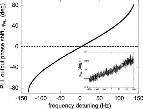
Figure 2: Phase shift between a $150$ kHz sinusoidal waveform sent to the real PLL and the PLL output waveform ($f_{\text{cent}}=150$ kHz) when tuning the input frequency from $-150$ to $+150$ Hz upon the frequency tracker is engaged or not. The 3kHz FIR low pass filter has been used. When the tracker is disengaged, the phase lag can reach $\pm 80$ degrees (continuous black line, amplitude of the input waveform : $A_{w}=110$ mV peak-to-peak). When it is engaged, the phase lag drops to almost zero (dotted black line and inset, similar input waveform). When the input frequency accurately matches the center frequency, the shift is zero (modulo an error corresponding to a few fractions of degrees as shown in the inset).

To assess how sensitive to frequency changes the phase is, the following experiment is carried out. A $150$ kHz sinusoidal waveform is generated by means of a function generator and sent to the real PLL. The frequency is then slowly detuned from $-150$ Hz up to $+150$ Hz. The phase lag between input and output waveforms, $\varphi_{\text{pll}}$, is recorded with a lock-in amplifier (Perkin Elmer 7280) and reported as a function of the detuning. The PLL center frequency is fixed to $f_{\text{cent}}=150$ kHz. The experiment is repeated the frequency tracker being engaged and disengaged. Two amplitudes of the PLL input waveform are used. In this experiment, the input waveform stands for the oscillatory motion of the cantilever and the tuning for the shift occurring when the tip is approached towards the surface upon attractive or repulsive forces. The results are reported in fig.2. When the tracker is disengaged, the maximum detuning corresponds to a phase lag of $\pm 80$ degrees, which means that the cantilever would then be driven off resonance severely. On the opposite, when engaged, the phase lag reduces (inset) to $\pm 0.05$ degree.

This feature has no consequence when the PLL is only used as a frequency demodulator like in the self-excitation mode. On the opposite in the PLL-excitation scheme, this point is crucial since the PLL is produces the excitation signal. Therefore particular attention has to be paid on the way it is produced. If it is abnormally phase shifted, then the oscillation amplitude drops and consequently apparent dissipation is generated, as shown in section V.

III.5 Block 5: phase shifter

The PS receives the $\sin$ and $\cos$ waveforms generated by the NCO. A further input to the block is the phase lag, $\varphi_{\text{ps}}$, fixed prior to starting the experiments to make the cantilever oscillating at $f_{0}$. The PS digitally computes :

$$z_{\text{ps}}(t_{i}) =\sin\left[\varphi_{\text{nco}}(t_{i})+\varphi_{\text{pll}}\right]\times\cos\left(\varphi_{\text{ps}}\right)$$

$$\text{~{}~{}~{}~{}~{}~{}~{}~{}~{}~{}~{}~{}~{}~{}~{}~{}~{}~{}~{}}+\cos\left[\varphi_{\text{nco}}(t_{i})+\varphi_{\text{pll}}\right]\times\sin\left(\varphi_{\text{ps}}\right)$$

$$=\sin\left[\varphi_{\text{nco}}(t_{i})+\varphi_{\text{pll}}+\varphi_{\text{ps}}\right]$$ (21)

When the system is being operated in the PLL-excitation mode, $z_{\text{ps}}(t)$ is converted into an analog signal by the DAC1 and multiplied by the APIC output.

III.6 Block 6: distance controller

The distance controller is the second digital PI controller implemented in the DSP operating at $f_{s_{3}}$. The block gets the setpoint value of the signal ($\Delta f$ or damping) onto which the control of the tip-sample distance is performed and the proportional and integral gains, $K_{p}^{\text{dc}}$ and $K_{i}^{\text{dc}}$, respectively. Here, let’s assume that the reference signal is the frequency shift, as depicted in fig.1. We have arbitrarily chosen not to describe the transfer function of the z-piezo drive. Therefore $K_{p}^{\text{dc}}$ and $K_{i}^{\text{dc}}$ have natural units (nm.Hz^-1 and nm.Hz^-1.s^-1, respectively). The controller is described by :

$$D(t_{i})= D(t_{\text{dc}})+K_{p}^{\text{dc}}\left[\Delta f_{\text{set}}-\Delta f(t_{i})\right]$$

$$+ \sum_{k>\text{dc}}^{i}{K_{i}^{\text{dc}}\left[\Delta f_{\text{set}}-\Delta f(t_{k})\right]\Delta t_{s_{3}}},$$ (22)

$D(t_{\text{dc}})$ being the tip-surface distance when the DPIC is engaged.

III.7 Lock-in amplifier

The description of the lock-in amplifier implemented in the simulation does not depict the detailed operational mode of the real lock-in which is used to monitor the phase shift of the oscillator (Perkin Elmer 7280). Its purpose is to provide an easy way to estimate the phase shift between the excitation and the oscillation. The calculation of the phase is performed at $2.5$ kHz. The buffer used to extract the phase therefore consists of $n_{\text{lock-in}}=f_{s_{1}}/2.5\text{~{}kHz}=8000$ samples. The numerical code used to describe it is :

$$\tan(\varphi(t_{i}))=$$

$$\frac{\sum_{k=i-n_{\text{lock-in}}}^{i}z_{\text{bpf}}(t_{k})\times\sin[\varphi_{\text{nco}}(t_{k})+\varphi_{\text{pll}}+\varphi_{\text{ps}}]}{\sum_{k=i-n_{\text{lock-in}}}^{i}z_{\text{bpf}}(t_{k})\times\cos[\varphi_{\text{nco}}(t_{k})+\varphi_{\text{pll}}+\varphi_{\text{ps}}]}$$ (23)

III.8 Code implementation

The numerical code has been implemented with LabView${}^{\text{TM}}$ $6.1$, supplied by National Instruments${}^{\text{TM}}$. It consists of a user interface where all the parameters are tunable at run-time, like during a real experiment. The couple of integro-differential equations 2, 3, 10, 11, 12, III.3, 14, 15, 16, III.5 and III.6 are integrated at their respective sampling frequencies. The monitored signals are the oscillation amplitude $A_{\text{rms}}$ (equ.11), the frequency shift $\Delta f$ (equ.17), the phase $\varphi$ (equ.III.7) and the relative damping $\Gamma/\Gamma_{0}-1$=$QK_{3}A_{exc}/A_{0}-1$, deduced from the APIC output (equ.4). The connection to the dissipated energy per cycle $E_{d}$ is given by equation 7, that is $\Gamma/\Gamma_{0}-1=E_{d}/E_{d_{0}}-1$.

IV Apparent dissipation vs. minimum dissipation

Addressing the question of apparent dissipation requires to estimate the minimum dissipation which is detectable by the instrument upon operating conditions. Beyond the specificities of the PLL- or self-excitation modes, important parameters like quality factor $Q$, temperature and bandwidth of the measurement must be considered.

We here focus on the minimum dissipated energy, $\delta E_{d}$, due to thermal fluctuations of the cantilever when it oscillates close to a surface. Thermal driving forces are connected to the energy dissipation by the $Q$ factor of the cantilever. The thermal kicks introduce fluctuations of amplitude and phase and therefore fluctuations of the energy dissipation. This is true for a free cantilever, but the contribution of the thermal noise is expected to be even more pronounced when the tip is close to the surface. Then, the fluctuations of the interaction force $\delta F_{\text{int}}$ have a strong influence on the nonlinear dynamics of the cantilever, in particular when the tip is at distances involving short-range forces where the nonlinearity is more pronounced.

The instrumental noise (cf. Ch.2 in refs.[morita02a, ] and [polesel05, ]), essentially due to electronic components, is not considered and we further assume that the electronic blocks (RMS-to-DC, PI controllers, PLL) operate perfectly. Doing so, $\delta E_{d}$ is under-estimated but the framework of this section is to provide a ground value to be compared to the values obtained with the simulation.

IV.1 Connection between $\delta E_{d}$ and $\delta F_{\text{int}}$

The fluctuation of the dissipated energy per cycle can be connected to the fluctuation of damping $\delta\Gamma$, via equ.7 :

$$\delta E_{d}=\pi k_{c}A_{0}^{2}\frac{\delta\Gamma}{\omega_{0}}$$ (24)

Besides, because $A_{\text{exc}}=A_{0}/Q=A_{0}\Gamma_{0}/\omega_{0}=F_{\text{exc}}/k_{c}$ on resonance and because the tip-sample interaction force $F_{\text{int}}$ can be treated, to first order note_virtual17 , on the same level as $F_{\text{exc}}$, a fluctuation of $F_{\text{int}}$ should produce, a fluctuation of damping :

$$\frac{\delta\Gamma}{\omega_{0}}=\frac{\delta A_{\text{exc}}}{A_{0}}=\frac{\delta F_{\text{int}}}{k_{c}A_{0}},$$ (25)

Consequently :

$$\delta E_{d}=\pi A_{0}\delta F_{\text{int}}$$ (26)

IV.2 Estimate of $\delta F_{\text{int}}$

For large oscillation amplitudes (that is larger than the minimum tip-surface distance, a few angströms), $F_{\text{int}}$ is connected to the so-called normalized frequency shift giessibl97a , $\gamma\equiv\Delta fk_{c}A_{0}^{3/2}/f_{0}$, via the equation ke99a (cf. also Ch.16 in ref.[morita02a, ]) :

$$\gamma(r)\simeq 0.43\sqrt{V_{\text{int}}(r)F_{\text{int}}(r)},$$ (27)

where $V_{\text{int}}(r)$ and $F_{\text{int}}(r)$ are the interaction potential and force, respectively, between the tip and the sample at a location $r$. The fluctuation in the relative frequency shift $\delta\Delta f/f_{0}=\delta f/f_{0}$, that is the cantilever frequency noise, due to a fluctuation of $F_{\text{int}}$ is then given by :

$$\frac{\delta f}{f_{0}}\simeq\frac{0.43}{2k_{c}A_{0}^{3/2}}\sqrt{\frac{V_{\text{int}}(r)}{F_{\text{int}}(r)}}\delta F_{\text{int}}$$ (28)

IV.3 Estimate of $\delta f/f_{0}$

Y. Martin et al. [martin87a, ], T.R. Albrecht et al. [albrecht91a, ], H. Dürig et al. [duerig97a, ] and F.J. Giessibl (Ch.2 in ref.[morita02a, ]) have calculated the thermal limit of the frequency noise in frequency-modulation technique over a measurement bandwidth $B$. It is given by :

$$\frac{\delta f}{f_{0}}=\sqrt{\frac{2k_{B}TB}{\pi^{3}k_{c}A_{0}^{2}f_{0}Q}}$$ (29)

Therefore, the dissipated energy due to thermal fluctuations of the cantilever close to the surface can be estimated to :

$$\delta E_{d}\simeq 4.6\sqrt{\frac{2k_{B}TBk_{c}A_{0}^{3}F_{\text{int}}(r)}{\pi f_{0}QV_{\text{int}}(r)}}$$ (30)

The measurement bandwidth $B$ can be estimated out of the following considerations. As mentioned by F.J. Giessibl (cf. Ch.2 in ref.[morita02a, ]), $B$ is a function of the scan speed $v_{s}$ and the distance $a_{0}$ between the features which need to be resolved :

$$B=\frac{v_{s}}{a_{0}}$$ (31)

For UHV investigations, $a_{0}$ is of about one atomic lattice constant, that is a few angströms. At room temperature, due to thermal drift, atomic scale images are usually recorded at scan speeds of about 6 lines (3 forwards plus 3 backwards) per second. Let’s consider for instance a moderate resolution of $6$ pixels per atomic period. Then, a line consisting of $256$ pixels should be acquired with a bandwidth $B=6\times 256/6=256$ Hz.

Table 1 gives some estimates of the relative dissipated energy due to thermal fluctuations of the cantilever $\delta E_{d}/E_{d_{0}}$ close to the surface in the short-range or pure Van der Waals regimes at various temperatures and for various quality factors. In UHV at room temperature, our experimental conditions, the minimum dissipated energy which is detectable corresponds to $5\%$ of the intrinsic dissipated energy of the free cantilever. This corresponds to about 150 meV/cycle with typical conditions for UHV investigations carried out at room temperature (cf. equ.7 and discussion below). Besides, as mentioned before, this value is underestimated. A straightforward consequence is that the strength of apparent dissipation should overcome this limit to be relevant. With a moderate quality factor in the Van der Waals regime like in high vacuum for instance, the limit drops by almost a factor 3 ($1.8\%$). Thus, apparent dissipation effects might occur more easily under these conditions note_virtual14 . At low temperatures, in the short-range regime the ratio is $2.67\%$. However, this value is likely still too high because then, the thermal drift being drastically reduced, the measurement bandwidth can be lowered and apparent dissipation more likely to be measured.

$Q$	Interaction	$E_{d_{0}}$	$\delta E_{d}$	$\delta E_{d}/E_{d_{0}}$
	regime	(eV/cycle)	(eV/cycle)
$5000$ ($298^{\circ}$K)	VdW + short-range	7.69	0.177	$2.3\%$
	VdW only	7.69	0.141	$1.8\%$
$30000$ ($298^{\circ}$K)	VdW + short-range	1.28	$7.25\times 10^{-2}$	$5.7\%$
	VdW only	1.28	$5.78\times 10^{-2}$	$4.5\%$
$500000$ ($4^{\circ}$K)	VdW + short-range	0.077	$2.06\times 10^{-3}$	$2.7\%$
	VdW only	0.077	$1.64\times 10^{-3}$	$2.1\%$

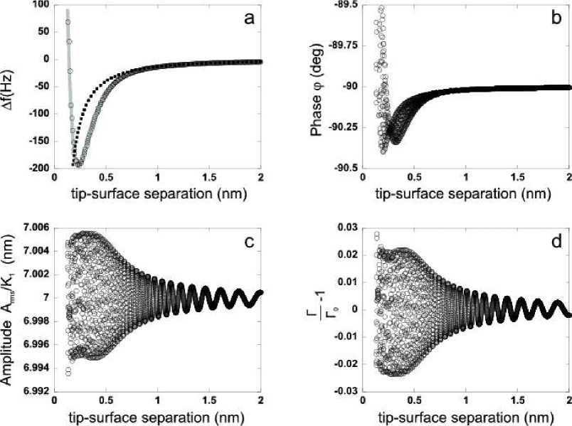
Figure 3: Numerical approach curves. The parameters are $A_{0}^{\text{set}}=7$ nm, $f_{0}=150$ kHz, $k_{c}=30$ N.m^-1, $Q=30000$, therefore $\Gamma_{0}=31.4$ s^-1 and $E_{d_{0}}=0.96$ eV/cycle, $K_{1}=0.1$ V.nm^-1, $K_{3}=1/K_{1}$ nm.V^-1, $K_{d}=1$ V, $K_{0}=5000$ rad.V^-1.s^-1, $K_{p}^{\text{ac}}=10^{-3}$, $K_{i}^{\text{ac}}=10^{-4}$ s^-1, approach speed $2$ nm.s^-1. The parameters of the interaction potential have been taken from ref.[47] : $H=1.865\times 10^{-19}$ J, $R=5$ nm, $U_{0}=3.641\times 10^{-19}$ J, $\lambda=1.2~{}\AA$, and $r_{c}=2.357~{}\AA$. Except in (a), the signals are monitored at $10$ kHz. (a)- Comparison between the $\Delta f$ computed numerically (open circles) and the analytic expression of $\Delta f$ (thick grey line) due to Van der Waals and Morse interactions (equ.46). The two curves match accurately along the attractive and repulsive parts of the interaction potential. For clarity reasons, 10 times less samples are displayed compared to plots shown in (b), (c) and (d). The dotted line depicts the analytic $\Delta f$ due to a pure Van der Waals potential, thus showing where the short- and long-range interaction regimes are discernable. (b)- Phase lag, $\varphi$. The frequency tracker being engaged, the phase remains constant and equal to $-90$ degrees within deviations limited to $0.3\%$, thus maintaining the cantilever driven on resonance. (c)- Amplitude $A_{\text{rms}}(t)/K_{1}$. Since no phase variation occur, the amplitude remains constant as well throughout the approach. (d)- Relative damping.

Table 1: Dissipated energy of the free cantilever $E_{d_{0}}$ (equ.7) and dissipated energy due to thermal fluctuations of the cantilever close to the surface $\delta E_{d}$ (equ.30) for various quality factors and temperatures when Van der Waals plus short-range (equ.9) or pure Van der Waals forces (similar equation, with $U_{0}=0$) are considered. The cantilever parameters are $A_{0}=7$ nm, $f_{0}=150$ kHz, $k_{c}=40$ N.m^-1 and $B=260$ Hz. The parameters of the interaction potential have been taken from ref.[perez98a, ] : $H=1.865\times 10^{-19}$ J, $R=5$ nm, $U_{0}=3.641\times 10^{-19}$ J, $\lambda=1.2~{}\AA$, and $r_{c}=2.357~{}\AA$. $\delta E_{d}$ has been estimated at a distance $r$ for which the two interaction regimes are clearly distinct (cf. fig.3(a)), $r=5$ $\AA$.

V Results

V.1 Validation of the numerical setup

Frequency shift vs. distance curves obtained from the simulation have first been compared to the analytic expression of $\Delta f$ due to Van der Waals and Morse potentials (cf. appendix, section A). The results are shown in fig.3(a). The parameters chosen to perform the simulation are consistent with typical parameters used during experiments performed in UHV. The parameters of the interaction potential have been taken from ref.[perez98a, ]. They are representative of the interaction between a silicon tip and a silicon(111) facet. An excellent agreement is observed between numerical and analytic curves along the attractive and repulsive parts of the interaction potential, thus validating the numerical scheme. The parameters used to perform the calculation are given in the caption. Let’s also notice that the frequency tracker was engaged. In figs. 3(b), (c) and (d), the variations of $\varphi$, $A_{\text{rms}}$ and relative damping, respectively are reported vs. the tip-surface separation. Phase and amplitude remain almost constant while approaching, within, however, deviations limited to $0.3\%$ compared to $-90$ degrees and $A_{0}^{\text{set}}=7$ nm, respectively. In the repulsive part of the potential, steep phase changes occur, but the amplitude does not dramatically drops, at least up to $\Delta f=+100$ Hz. Consequently, the relative damping remains constant.

V.2 Numerical vs. real setups

V.2.1 PLL dynamics

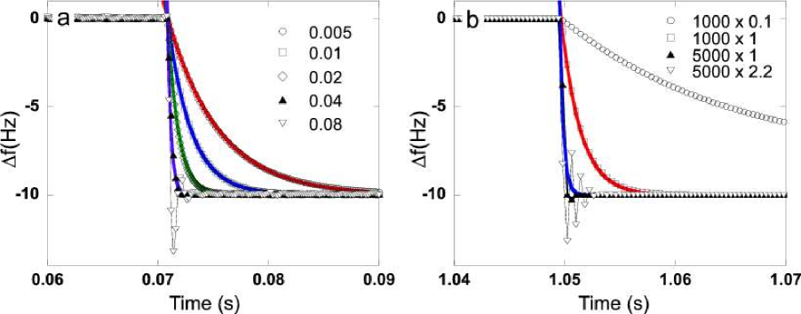
Figure 4: (Color online) Step response of the real (a) and of the simulated (b) PLLs to a center frequency step of $+10$ Hz at $f_{\text{cent}}=150$ kHz, resulting in a $\Delta f$ of $-10$ Hz. For this experiment, no interaction between the tip and the surface occurs. The various curves represent the experiments carried out for various values of the related gains of the PLLs denoted by the symbols. The PLL output is recorded at $10$ kHz. The curves are fitted with a decaying exponential (thick continuous lines) out of which the PLL “locking time” is extracted. They are displayed over similar relative ranges.

The dynamic behaviors of real and simulated PLLs have then been compared. The experiment consists in locking the PLL onto a $150$ kHz sinusoidal waveform according to the same procedure than in section III.4.5. The $3$ kHz FIR low pass filter is used. At a certain moment, a frequency step of $+10$ Hz is applied to the center frequency, resulting in a shift of $-10$ Hz ($\omega_{0}+2\pi\Delta f=\omega_{\text{cent}}$). The step response is recorded for various values of the so-called loop gain (real PLL) and various values of $K_{0}K_{d}$ (simulation). The variations of $\Delta f$ vs. time are fitted with simple decaying exponential functions, the characteristic time of which stands for the locking time of the PLL. The results are reported in figs.4(a) and (b). A rather long locking time is noticed for low values of the gains whereas the PLLs lock faster when the gains become larger. For the latter case, the PLLs can operate up to the limit of the locking range as shown by the oscillations.

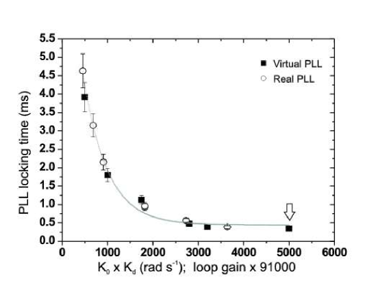
Figure 5: Locking time of the simulated (filled squares) and real (empty circles) PLL vs. $K_{0}K_{d}$ and loop gain$\times 91000$. The locking times are obtained from the related step response curves (figs.4(b) and (a), respectively). The error bars depict the uncertainty on the fitted value of the locking time ($\pm 10\%$). The arrow indicates the value of the loop gain used experimentally which corresponds to an optimum behavior of the PLL and a related locking time of about 0.35 ms. The curve is given as guide eyes.

The locking time deduced from each fit is plotted as a function of the gains of both PLLs. In order to make the curves comparable, the loop gain must be rescaled by an arbitrary constant which depends on the electronics. The best agreement between the curves was achieved with $91\times 10^{3}$ (cf. fig.5). A single master curve of the PLL dynamics can thus be extracted. The rather good agreement between the two curves provides evidence that the simulation reasonably describes the real component, at least within the locking range. For values of the gains up to $K_{0}K_{d}=6000$ rad.s^-1, the PLL is stable and able to track frequency changes within the locking range around $150$ kHz. Above 6000 rad.s^-1, the PLL introduces overshoot in the output waveform while attempting to lock the input signal. For higher gains, the PLL is not able to properly track the input signal, even though its frequency is within the locking range. The border is reached for $K_{0}>10^{4}$ rad.V^-1.s^-1, in good agreement with the value expected from R.Best’s criterion (cf. discussion in section III.4.4). The arrow in fig.5 indicates the usual loop gain value which is chosen to perform the experiments using the $3$ kHz low pass filter, corresponding to $K_{0}K_{d}=5000$ rad.s^-1. The related locking time of the PLL is then $\simeq 0.35$ ms. For those values of gains, the locking range is about $\pm 400$ Hz.

V.2.2 APIC dynamics

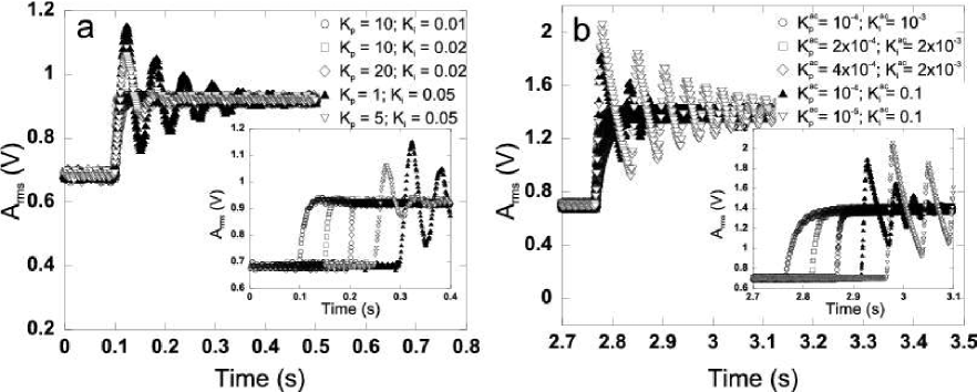
Figure 6: Step response of the real (a) and of the simulated (b) APIC to a $A_{0}^{\text{set}}$ step. To perform the experiments, the related PLLs are engaged (frequency trackers as well). The $3$ kHz FIR low pass filter has been used. No interaction between the tip and the surface occurs. The cantilever properties are $f_{0}=157514.6$ Hz and $Q=36000$. To perform the calculation, since the cantilever stiffness was not accurately known, we have arbitrarily chosen $k_{c}=30$ N.m^-1, in reasonable agreement with manufacturer’s datasheet. The other numerical parameters are similar to those given in fig.3. The curves depict the experiments carried out for various values of $K_{p}^{\text{ac}}$ and $K_{i}^{\text{ac}}$ gains. Three behaviors are observed : overcritically damped responses without overshoot, critically damped responses with a slight overshoot and undercritically damped responses with an oscillating behavior. The insets show them for couple of curves which have been arbitrarily shifted along the time axis, but note that the relative ranges are similar.

In order to extract a typical time constant of the component, similar experiments have been carried out with the APICs. The cantilever remaining far from the surface, a step is applied to the setpoint amplitude $A_{0}^{\text{set}}$ resulting in an abrupt change in $A_{\text{rms}}$ upon gains. The results are reported in fig.6(a, real setup) and (b, simulated setup). The curves exhibit over- (no overshoot at all) under- (oscillating behavior) or critically damped (single overshoot) behaviors upon chosen gains. So as to extract the APIC response time, we focus at curves which exhibit a single time constant, that is curves for which a weak overcritically or a critically damped response is observed (cf. insets in figs.6(a) and (b)). This is motivated by the controller response which is then the fastest, while preserving an overall stable behavior. The changes in $A_{\text{rms}}$ are fitted with decaying exponentials functions and the related characteristic time is extracted. The variation of the so-called response time of the controller ($t_{\text{resp}}$) vs. gains is reported in fig.7. The restriction to curves exhibiting a single time constant is similar to restricting the analysis to a single gain of the controller note_virtual18 . Thus, a single master curve which describes the dynamics of both APICs can be extracted as well. In fig.7, the $K_{p}$ gain of the real controller has been rescaled to make it matching $K_{p}^{\text{ac}}$ (the best rescaling factor is 1/40000). $t_{\text{resp}}$ decreases as $K_{p}^{\text{ac}}$ increases (being given a single $K_{i}^{\text{ac}}$ per $K_{p}^{\text{ac}}$). However, the controller is limited to an optimum $t_{\text{resp}}$ of about $2$ ms as shown by the plateau reached for $K_{p}^{\text{ac}}\simeq 10^{-3}$ [note_virtual01, ] (arrow in fig.7).

So far, the origin of the saturation remains unclear. Nevertheless, a brief analysis of the response function of the controller to a step wherein the contribution of the RMS-to-DC converter is neglected (cf. appendix, section B) emphasizes that the dynamic behavior can reasonably be predicted (triangles in fig.7) up to $2$ ms. The best agreement between the experimental results and the model is found when considering the weak overcritically damped regime, namely :

$$t_{\text{resp}}\simeq\frac{1}{c+\sqrt{c^{2}-\frac{\omega_{0}}{2}K_{1}K_{3}K_{i}^{\text{ac}}}},$$ (32)

with :

$$c=\frac{\omega_{0}}{4}\left(\frac{1}{Q}+K_{1}K_{3}K_{p}^{\text{ac}}\right)$$ (33)

The origin of the saturation might thus be attributed to the contribution of the RMS-to-DC converter.

As expected, the shortest APIC response time is approximately $6$ times longer than the optimal PLL locking time, $\simeq 0.35$ ms. Thus the PLL should track frequency changes much faster than amplitude changes. Therefore, with PLL gains insuring a locking time much shorter than the APIC one, the two blocks can be considered as operating separately. Then, no amplitude changes which would be the consequence of a bad tracking of the resonance frequency can occur.

It might be objected that the experiments and the analysis, despite consistent, have been performed without considering the tip-sample interaction. Regarding the PLL, the way the dynamics is affected when the tip is close to the surface has not yet been investigated. But regarding the amplitude controller, Couturier et al. [couturier03a, ] have reported a theoretical analysis of the controller stability upon the gains and the strength of the non-linear interaction in the self-excitation scheme. The analysis stresses that the stability domain of the controller shrinks when the contribution of the non-linear interaction (pure Van der Waals) increases. Thus, a couple ($K_{p}^{\text{ac}}$;$K_{i}^{\text{ac}}$) initially inside the stability domain might correspond to an unstable behavior of the controller close to the surface, thus introducing apparent dissipation couturier03a . Nevertheless, considering their parameters with a tip-surface distance ranging from infinity down to $0.8$ $\AA$ (corresponding to $\Delta f\lesssim-250$ Hz), that is very close to the surface for operating in nc-AFM note_virtual07 , the stability domain weakly shrinks note_virtual06 . A similar analysis for the PLL-excitation scheme is still lacking and should be performed for quantitative comparison and discussion. But comparing their analysis to the tip-surface distances and frequency shifts which are being used in this work, we believe that the contribution of the non-linear interaction to the APIC dynamics remains weak and thus would not change drastically its coupling to the PLL. This point is strengthened by the results given in the following section (V.3.1).

V.3 Apparent dissipation

V.3.1 Contribution of the PLL gains

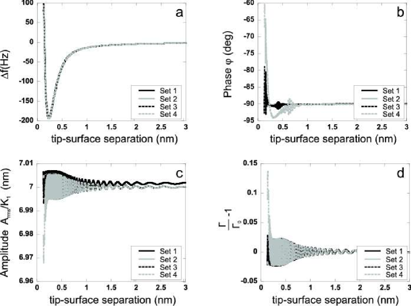
Figure 8: Approach vs. distance curves for various sets ($1$ to $4$) of $K_{0}K_{d}$ of the Pll gains, namely : $11000$ (continuous black line), $5000$ (continuous grey line), $1000$ (dotted black line) and $100$ rad.s^-1 (dotted grey line), corresponding to locking times of 0.2, 0.35, 1.8 and $>4$ ms, respectively. (a)- $\Delta f$, the curves are all matching each other. (b)- Phase lag $\varphi$, (c)- amplitude $A_{\text{rms}}(t)/K_{1}$ and (d)- relative damping. Except $K_{0}K_{d}$, the parameters are similar to those given in fig.3, in particular $K_{p}^{\text{ac}}=10^{-3}$ and $K_{i}^{\text{ac}}=10^{-4}$ s^-1 corresponding to $t_{\text{resp}}\simeq 2$ ms. When the PLL locking time is larger than $t_{\text{resp}}$ (set $4$, $K_{0}K_{d}=100$), the resonance is not properly locked, which induces a phase shift. Consequently, the amplitude decreases and the damping increases.

Section V.2.1 has proved that the PLL gains were controlling the PLL locking time. Within the locking range, the higher $K_{0}K_{d}$, the faster the PLL. The test performed here is to compute approach curves for various values of $K_{0}K_{d}$. Except $K_{0}K_{d}$, the parameters are similar to those given in fig.3. In particular, $Q=30000$, $K_{p}^{\text{ac}}=10^{-3}$ and $K_{i}^{\text{ac}}=10^{-4}$ s^-1, corresponding to $t_{\text{resp}}=2$ ms. $4$ sets of $K_{0}K_{d}$ have been used, namely : $11000$, $5000$, $1000$ and $100$ rad.s^-1, corresponding to locking times of $\simeq 0.2$ ms, $0.35$ ms, $1.8$ ms and $>4$ ms, respectively. Note that the two later values are almost similar or larger, respectively, than $t_{\text{resp}}$. The $3$ kHz FIR low pass filter has been used and the frequency tracker has been engaged. The results are reported in fig.8.

With the four sets of data, no effect on the frequency shift is observed. For $K_{0}K_{d}=11000$ and $5000$ rad.s^-1, changes in phase, amplitude and damping are noticeably similar. The phase and the amplitude remain constant and subsequently, no damping occurs. On the opposite, for $K_{0}K_{d}=1000$ and $100$ rad.s^-1, that is for a PLL locking time of about or larger than the APIC one, the changes are more pronounced. With $K_{0}K_{d}=1000$ rad.s^-1 (set 3), the phase strongly varies along the repulsive part of the interaction, from $-93$ to $-79$ degrees. Consequently, the amplitude starts dropping and the damping increases. This trend is more pronounced with $K_{0}K_{d}=100$ rad.s^-1, for which the phase in the repulsive regime reaches $-60$ degrees, requiring the APIC to produce $\simeq 14\%$ more excitation. According to the discussion put forward in section IV, such an effect is expected to be detected if it would occur.

Therefore, if the PLL does not lock the incoming signal fast enough, that is for locking times of about or larger than $1$ ms, corresponding approximately to $t_{\text{resp}}/2$, an undesirable phase shifted signal is produced, resulting in an amplitude decrease and producing significant apparent dissipation.

It’s peculiar to notice that, when the cantilever is driven out of resonance as shown with the phase changes with $K_{0}K_{d}=100$ rad.s^-1, no abnormal frequency shift occurs. As a matter of fact, close to the resonance, the phase changes of the free cantilever scale as, to first order : $\varphi\overset{u\rightarrow 1}{=}\pi/2-2Q(u-1)$, where $u=f/f_{0}$. Considering $f_{0}=150$ kHz and $\delta\varphi=\pm 30$ degrees, then $\delta f=f_{0}\delta\varphi/2Q=\pm 1.3$ Hz, which is not visible in fig.8(a). Similar effects have been reported by H.Hölscher et al. [hoelscher01a, ]. This effect should be more (less) pronounced with low (high) $Q$ values ($\pm 8$ Hz or $\pm 0.08$ Hz with $Q=5000$ or $500000$, respectively) and the apparent dissipation higher (lower).

V.3.2 Contribution of the frequency tracker

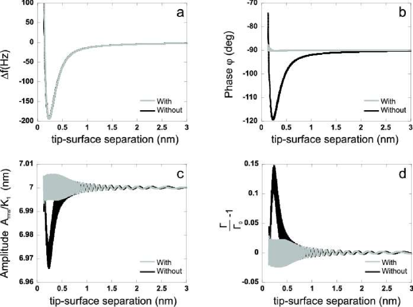
Figure 9: Approach vs. distance curves upon the frequency tracker of the PLL is engaged or not (grey or black lines, respectively).(a)- Frequency shift $\Delta f$, (b)- phase lag $\varphi$, (c)- amplitude $A_{\text{rms}}(t)/K_{1}$ and (d)- relative damping. The parameters are similar to those given in the caption of fig.3. When not engaged, the phase continuously drifts during the approach due to the increase of the attractive interaction meaning that the oscillator is not driven on resonance. Subsequently, the amplitude drops and the APIC strives to keep it constant by increasing the excitation. $15\%$ more excitation is thus produced, that is above thermal noise (cf. section IV).

As mentioned in paragraph III.4.5, the frequency tracker updates $\omega_{\text{cent}}$ with the goal to prevent the phase due to the frequency shift, $\varphi_{\text{pll}}$, be added to the NCO output. Figure 9 reports two approach curves computed upon the frequency tracker is engaged or not. When it is disengaged, the phase continuously decreases along the attractive part of the interaction potential, as expected from equ.20. At a tip-sample separation corresponding to the minimum of the interaction potential, $r=2.35$ $\AA$, the phase reaches $-120$ degrees, meaning that the oscillator is then seriously driven out of resonance. Following the phase change, the amplitude continuously decreases and the damping strives to compensate the amplitude reduction, thus reaching $15\%$ of the intrinsic damping of the free oscillator. Here again, such an effect should be measurable. When the tip is further approached towards the surface, the repulsive regime makes the frequency shift increasing and so does $\varphi_{\text{pll}}$. The amplitude increases back to reach $A_{0}^{\text{set}}$ and the damping is obviously reduced. An amplitude growth is not expected in the repulsive region of the interaction potential, but it is the consequence of the bad tracking of the resonance frequency. On the other hand, when the tracker is engaged, as already mentioned, the phase remains constant and no apparent dissipation occurs.

V.4 Scan lines

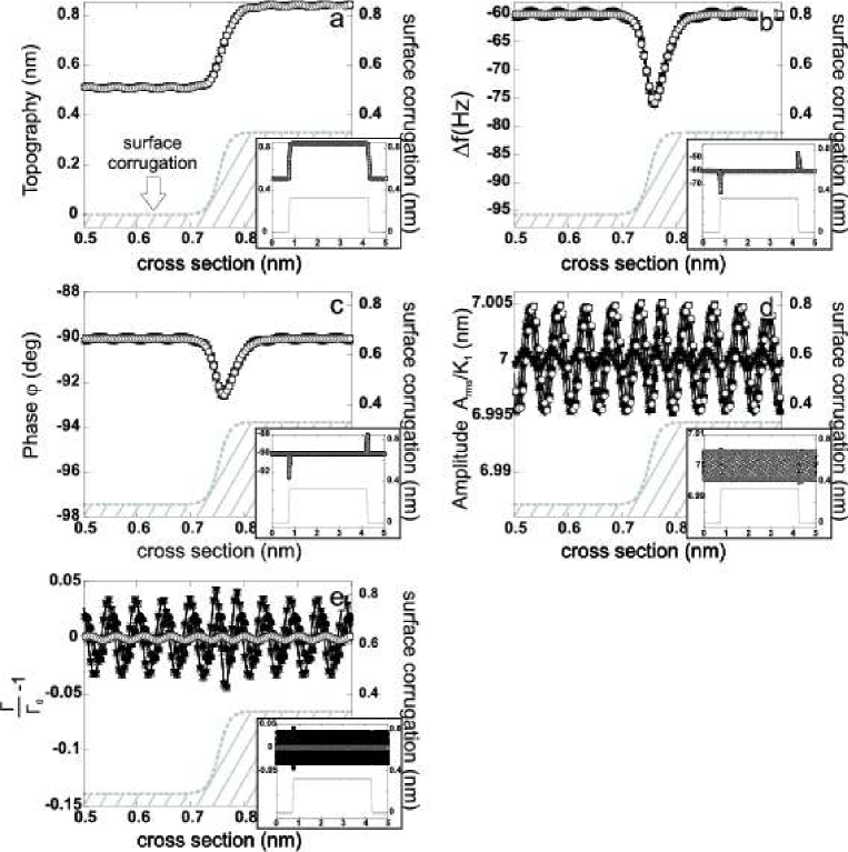
Figure 12: Calculated cross-section of a surface with two opposite steps for various sets of the APIC gains, namely $(K_{p}^{\text{ac}}=10^{-2};K_{i}^{\text{ac}}=10^{-3}$ s${}^{-1})=\circ$, $(10^{-3};10^{-3})=\diamond$, $(10^{-2};10^{-2})=\times$, $(10^{-3};10^{-2})=+$, $(10^{-2};10^{-4})=\vartriangle$, $(10^{-3};10^{-4})=\bullet$, $(10^{-4};10^{-4})=\blacksquare$, $(10^{-4};10^{-3})=\blacklozenge$, $(10^{-3};10^{-5})=\blacktriangle$, $(10^{-2};10^{-5})=\blacktriangledown$ and $(10^{-4};10^{-5})=\odot$. The scan lines have been initiated upon the same conditions than in fig.10 with $K_{0}K_{d}=5000$ rad.s^-1. The lateral scan speed is $5$ nm.s^-1 and the section consists of 1024 samples. The gains of the distance controller are similar to those given in fig.10. (a)- Topography. (b)- Frequency shift. (c)- Phase lag $\varphi$. (d)- Amplitude $A_{\text{rms}}/K_{1}$ and (e)- relative damping. The APIC gains have a negligible effect on the topography. A weak apparent damping ($3\%\Gamma_{0}$, that is not experimentally relevant) is revealed at the step if the APIC is slow, corresponding to $t_{\text{resp}}=20$ ms.

In addition to the analysis of the time constant of the various blocks, it is important to focus at variables changes when the tip is scanned along a surface. Two types of surfaces have been investigated : 1- a sinusoidally corrugated surface with a spatial wavelength of $6.6~{}\AA$ and a corrugation of $\pm 0.1$ nm, consistently with the lattice constant of KBr, a sample regularly used in the group, and 2- a surface with two opposite steps with a step height of $3.3~{}\AA$. The steps are built out of $\arctan$ functions and spread out laterally over $5~{}\AA$. The upper terrace spreads out over $3$ nm (cf. insets in fig.12).

The results shown here have all been obtained by $\Delta f$ regulation. The scan lines have been initiated from the approach curve shown in fig.3 with $\Delta f_{\text{set}}=-60$ Hz, corresponding to an initial tip-surface separation of about $5~{}\AA$, that is in the short-range regime (cf. fig.3(a)). The gains of the distance controller have been chosen in order to insure a critically damped response of the controller to a step of $-1$ Hz when $\Delta f_{\text{set}}$ is reached, namely $K_{p}^{\text{dc}}=2\times 10^{-3}$ nm.Hz^-1 and $K_{i}^{\text{dc}}=2$ nm.Hz^-1.s^-1. For all of the following curves, the frequency tracker has been engaged. Three sets of parameters have been varied : the PLL gains, the scan speed and the APIC gains.

V.4.1 Contribution of the PLL gains

Paragraph V.2.1 has proven how $K_{0}$ and $K_{d}$ gains were controlling the PLL locking time. Figure 10 shows scan lines computed for three values of $K_{0}K_{d}$, namely : $100$, $1000$ and $5000$ rad.s^-1, corresponding to locking times $>4$, $1.8$ and $0.35$ ms, respectively. The unchanged parameters are : scan speed $=7$ nm.s^-1, $K_{p}^{\text{ac}}=10^{-3}$ and $K_{i}^{\text{ac}}=10^{-4}$ s^-1. The latter gains correspond to $t_{\text{resp}}\simeq 2$ ms (arrow in fig.7). Each signal, namely topography, $\Delta f$, $\varphi$, $A_{\text{rms}}$ and relative damping, consists of 256 samples. The topography signal follows accurately the surface corrugation. No contribution due to the gains is revealed. $\Delta f$ is modulated around $\Delta f_{\text{set}}=-60$ Hz, with an amplitude ranging from $\pm 2$ to $\pm 3$ Hz upon $K_{0}K_{d}$. The accuracy of the distance control is then of about $97\%$. Note also that the nonlinear interaction makes the modulation asymmetric around $\Delta f_{\text{set}}$ and the maxima are mismatched compared to the maxima of the surface. However, the mismatch does not depend on $K_{0}K_{d}$. If the PLL is slow, a rather important phase lag is observed, ranging from $-65$ to $-110$ degrees, resulting in small amplitude changes. Here also, the asymmetry around $-90$ degrees is manifest and it’s interesting, despite expected, to notice the doubling in the periodicity of the amplitude fluctuation. The related relative apparent damping fluctuates accordingly, reaching about $12\%\Gamma_{0}$, which should be experimentally detectable.

V.4.2 Contribution of the scan speed

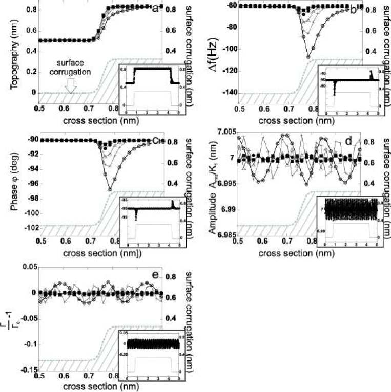
Figure 11: Calculated cross-section of a surface with two opposite steps for various scanning speeds, namely 1 ($\blacksquare$), 2 ($\bullet$), 5 ($\vartriangle$), 10 ($+$) and 20 nm.s^-1 ($\circ$). For clarity reasons, the right hand side step region has been magnified. The insets show the whole section. The scan lines have been initiated upon the same conditions than in fig.10 with $K_{0}K_{d}=5000$ rad.s^-1, $K_{p}^{\text{ac}}=10^{-3}$ and $K_{i}^{ac}=10^{-4}$ s^-1. The high speeds require to reduce the number of samples per line to 256. The gains of the distance controller are similar to those given in fig.10. (a)- Topography. (b)- Frequency shift. (c)- Phase lag $\varphi$. (d)- Amplitude $A_{\text{rms}}/K_{1}$ and (e)- relative damping. At high scan speeds, the topography is slightly distorted, but the overall damping remains weak and below the thermal noise (cf. section IV).

Five scan speeds ranging from $1$ to $20$ nm.s^-1 have been used, accordingly to typical experimental values for such a scan size. The unchanged parameters are : $K_{0}K_{d}=5000$ rad.s^-1, $K_{p}^{\text{ac}}=10^{-3}$ and $K_{i}^{\text{ac}}=10^{-4}$ s^-1. The surface with opposite steps has been used and each signal consists of 256 samples. The results are given in fig.11. At high speed, the topography channel starts being distorted as a consequence of a bad distance regulation as shown by the large $\Delta f$ variations. The phase varies accordingly, but within a narrower domain. Therefore neither relevant variations of amplitude nor of relative damping ($\pm 2\%$ only) are revealed.

V.4.3 Contribution of the APIC gains

Similar experiments have been carried out by varying the APIC gains. Thirteen sets of $K_{p}^{\text{ac}}$ and $K_{i}^{\text{ac}}$ values have been used over 2 orders of magnitude for each gain. The unchanged parameters are : scan speed $=5$ nm.s^-1 and $K_{0}K_{d}=5000$ rad.s^-1. The surface with opposite steps has been used. For those curves, each signal consists of 1024 samples. The sets of gains have been chosen such that the response time of the controller is varied from $2$ to $20$ ms, according to fig.7. The results are reported in fig.12. Here again, the topography signal accurately follows the corrugation. In particular, no unwanted overshoot is observed at the step edge despite $\Delta f$ varies significantly. A small phase variation is observed at the step edge. For the latter three channels, no dependence is observed upon the gains such that the curves match each other. The small phase variation induces a tiny amplitude change, barely visible in the inset of fig.12(d), but the overall fluctuations are weak, which corresponds to relative damping fluctuations of $\pm 3\%$ (worse case, $t_{\text{resp}}\approx 20$ ms). Following discussion of section IV, this value is below the threshold limit of thermal noise, at least for experiments carried out in UHV and at room temperature. Upon gains, a small spatial shift is observed in the amplitude or in the relative damping signals up to a maximum value of $0.1$ $\AA$.

VI Discussion

The above analysis stresses five important results :

• The PLL dynamics plays a major role in the occurrence of relevant apparent damping if the locking time is about or larger than 1 ms, that is only twice faster than the APIC optimum response time. By “relevant damping”, we mean, on the base of the discussion given in section IV, a damping which would be detectable experimentally upon operating conditions (cf. table 1).

• The frequency tracker, the aim of which is to update the PLL center frequency to make it matching the actual resonance frequency, plays also a major role in the occurrence of apparent damping. It has to be mandatorily engaged when performing approach-curves, otherwise unwanted additional phase shift due to the PLL occurs and the cantilever is then driven off resonance.

• The PLL optimal locking time is about $0.35$ ms that is 6 times shorter than the shortest APIC response time of the free cantilever. Therefore the resonance condition is expected to be always properly maintained. Consequently, when the PLL operates properly, no amplitude changes due to a bad tracking of the resonance frequency are expected to occur. If they would, this should rather be the consequence of the APIC and/or the DPIC dynamics.

• The APIC response time seems to be limited to $t_{\text{resp}}\simeq 2$ ms due to the RMS-to-DC converter. There is a priori no fundamental restriction to the APIC response time, as shown by fig.7. However, it must be stressed that if the APIC is made faster, the PLL should be made faster accordingly.

• A weak contribution of the APIC to apparent dissipation is observed. Although spatial shift and apparent dissipation can conditionally be generated, the overall strength of the effect remains weak and should hardly be measurable for UHV investigations at room temperature.

In order to compare our results to other works, the contribution of the noise (equ.30) to the dissipation has been estimated with the parameters given by Gauthier et al. [gauthier02a, ]. The maximum of relative apparent damping they report is about $5\%$ (cf. fig.4 in the above reference, curve $\sharp$6), corresponding to a scanning speed of about $90~{}\AA$.s^-1. The spatial wavelength of their surface model being $8\AA$, the bandwidth of the corresponding measurement is $B\simeq 11$ Hz (cf. equ.31). The non-linear interaction is depicted by a Rydberg function with $U_{0}=4\times 10^{-11}$ J, $\lambda=0.599~{}\AA$ and $r_{c}=3~{}\AA$. With $A_{0}=1.5$ nm, $f_{0}=159154$ Hz, $k_{c}=26$ N.m^-1, $Q=24000$ ($E_{d_{0}}=4.8\times 10^{-2}$ eV/cycle), we get $\delta E_{d}/E_{d_{0}}\simeq 2.3\%$ at a distance note_virtual09 $s=4~{}\AA$. Therefore, due to the use of a low amplitude note_virtual15 , the strength of the effect would not be balanced by the noise and could be detectable experimentally. On the opposite, considering smaller scan speeds, the maximum of apparent dissipation decreases down to $2\%$. Such effects become then unlikely to be observed experimentally.

Finally, let’s note that the contribution of the third controller, the DPIC, has not been assessed in this work. Nevertheless, as mentioned by H. Hug and A. Baratoff [note_virtual08, ], in order to minimize feedback errors and resulting image distortions, the time constant of the distance controller must be shorter than the speed in the fast scanning direction / lateral extent of the smallest feature to be resolved and necessarily (much) larger than other time constants (RMS-to-DC, APIC, PLL). If those conditions are satisfied, then its contribution to the overall stability of the setup should be weak. This is what is readily seen in figs.10, 12 and, to a certain extend in fig.11, with reasonable speeds. This is also confirmed by Couturier et al. who have recently found out that the distance controller had no effect on the stability diagram in the self-excitation scheme and that only the amplitude controller played a role note_virtual05 ; couturier05a .

To summarize, this analysis has emphasized that a maximum of about $15\%$ of apparent dissipation, mainly due to the PLL and not to the APIC, could be generated (cf. fig.10). The contribution of the APIC, within the range of gains used, is systematically smaller. We finally infer that, with our setup (UHV and room temperature) and under typical experimental conditions (scanning speed, PLL and APIC gains…) corresponding to $E_{d_{0}}\simeq 2$ eV/cycle, apparent dissipation in the range of a few eV per cycle, as frequently reported in the literature, is unlikely to occur. A striking example is provided by R. Hoffmann et al. [hoffmann03a, ] who put in evidence a dissipation of 3 eV/cycle on a NiO(001) sample, despite operating at 4 K [note_virtual10, ]. This strongly suggests the interpretation of the experimental damping images in terms of “physical” dissipation.

VII Conclusion

The realization and successful testing of a modular nc-AFM simulator implemented with LabView${}^{\text{TM}}$ is reported. The design is based on a real electronics which includes a digital PLL, the output of which is used to detect the frequency shift but also to generate the time dependent phase of the excitation signal. Good agreement is obtained between the locking behavior of the real PLL and the PLL from the simulator. The optimum locking time of the PLL is found to be about 0.35 ms. The behavior of the amplitude controller is also found to correctly describe the real setup with an optimum response of 2 ms. The analysis of the time constants of the former two components provides evidence that the electronics tracks properly the cantilever dynamics if the PLL runs more than twice faster than the amplitude controller. When the system is operated with properly chosen parameters, frequency shift vs. distance curves successfully compare to an analytic expression which ignores the finite response of the electronics. No phase deviation resulting in apparent dissipation occur if the center frequency of the PLL tracks the resonance frequency shifted by the tip-sample interaction. An estimate of the minimum dissipation expected to be detected experimentally gives some insights on the relevance of apparent dissipation which can conditionally be generated numerically. This provides a framework to discuss the overall contribution of apparent dissipation during experiments. Computations of scan lines show that when the system is operated with experimentally relevant parameters, the contribution of the proportional and integral gains of the amplitude controller and the scan speed (up to $20$ nm.s^-1) do not lead to significant apparent dissipation. To give orders of magnitude, the worse situation (frequency tracker disengaged) leads to a maximum of $15\%$ more dissipation than the intrinsic dissipation of the free cantilever. This is below the values which are experimentally reported. This strongly suggests that nc-AFM damping images mainly reflect physical channels of dissipation and not electronics artifacts.

Besides Ref.couturier05a , two publications dealing with the implementation and/or performance of “virtual force microscopes” have appeared recently. These simulation codes are analogous to ours but differ in detail. Kokavecz et al.kokavecz06a proposed and tested a numerical scheme designed to produce response times of the whole simulated setup, as well as of separate blocks (amplitude, phase and distance controllers) as short as 0.1 ms. Trevethan et al.trevethan06a used the scheme described in Ref. polesel05 to compute fingerprint-like responses in the frequency shift, the minimum tip-sample distance and the damping signal caused by an atomic-scale configuration change at the surface of the sample. This change was first predicted from atomistic simulations and then induced upon approach under distance control down to a judiciously chosen frequency setpoint. A manual describing the combined atomistic simulationkantorovich04a and virtual force microscope codes is now available onlinenote_virtual19 .

Appendices

VII.1 The analytical method

The analytical method gives analytical, tractable expressions of the frequency shift versus distance upon the force expression. Couple of years ago, F.J. Giessibl and M.Guggisberg have proposed approached expressions for the frequency induced by a Morse potential [42, 6]. Here a complete expression is provided. The following calculation is based on a variational method extensively detailed in former articles [58]. We start from equation 2 and postulate a solution of the differential equation where the amplitude and the phase are not constant, but are allowed to vary slowly within time, that is over durations much longer than the oscillating period, namely :

$$z(t)=A(t)\cos\left[\omega t+\varphi(t)\right]$$ (34)

Equation 2 is then equivalent to :

$$\left\{\begin{array}[]{ll}\alpha\cos\left(\varphi(t)\right)-\beta\sin\left(\varphi(t)\right)=\gamma\\ \beta\cos\left(\varphi(t)\right)+\alpha\sin\left(\varphi(t)\right)=0\end{array}\right.$$ (35)

with :

$$\left\{\begin{array}[]{lll}\alpha=\ddot{A}(t)+\frac{\omega_{0}}{Q}\dot{A}(t)+\left\{\omega_{0}^{2}-\left[\omega+\dot{\varphi}(t)\right]^{2}\right\}A(t)+\frac{2}{m}\tilde{F_{c}}\\ \beta=A(t)\ddot{\varphi}(t)+\left[2\dot{A}(t)+\frac{\omega_{0}}{Q}A(t)\right]\left[\omega+\dot{\varphi}(t)\right]+\frac{2}{m}\tilde{F_{d}}\\ \gamma=\omega_{0}^{2}K_{3}A_{exc}\end{array}\right.$$ (36)

$\tilde{F_{c}}$ and $\tilde{F_{d}}$ are the first Fourier components of the conservative and dissipative forces experienced by the tip over one oscillation period $T$, respectively :

$$\tilde{F_{c}}=\frac{1}{T}\partial_{A}\left\{\int_{0}^{T}{V_{\text{int}}(t)dt}\right\}$$ (37)

$$\tilde{F_{d}}=\frac{1}{TA}\partial_{\varphi}\left\{\int_{0}^{T}{V_{d}(t)dt}\right\}$$ (38)

Setting $\dot{A}(t)=\ddot{A}(t)=\dot{\varphi}(t)=\ddot{\varphi}(t)=0$ yields to the steady equations of the oscillator in amplitude and phase out of which the relevant variables, namely $\Delta f=f-f_{0}$ and driving amplitude, related to the damping, can be extracted :

$$\tilde{F_{c}}=k_{c}A\left(\frac{\Delta f}{f_{0}}-\frac{f+2f_{0}Q\frac{\tilde{F_{d}}}{k_{c}A}}{2f_{0}Q\tan(\varphi)}\right)$$ (39)

$$\tilde{F_{d}}=\frac{k_{c}Af}{2f_{0}}\left(\frac{K_{3}A_{\text{exc}}}{A\left(1+\frac{\Delta f}{f_{0}}\right)\left(1+1/\tan(\varphi)\right)}-\frac{1}{Q}\right)$$ (40)

Equation 39 illustrates that, if the phase is properly maintained at $-\pi/2$ rad, the frequency shift is essentially due to the conservative interaction, whatever the dissipative contribution. Besides, equ.39 gives the well known expression of the frequency shift due to the conservative contribution [59] :

$$\frac{\Delta f}{f_{0}}=\frac{\tilde{F_{c}}}{k_{c}A}$$ (41)

The expression of $\tilde{F_{c}}$ related to the Morse potential given in equ.9 can be integrated analytically :

$$S_{\text{int}}^{\text{Morse}}=\int_{0}^{\frac{2\pi}{\omega}}V_{\text{int}}^{\text{Morse}}(t)dt=-\frac{2\pi U_{0}}{\omega}\left(2\Upsilon_{0,1/\lambda}-\Upsilon_{0,2/\lambda}\right),$$ (42)

where :

$$\Upsilon_{\alpha,\beta}=e^{-\beta(D-r_{c})}\times\text{BesselI}(\alpha,\beta A)$$ (43)

$\text{BesselI}(\alpha,\beta A)$ is the modified Bessel function of first kind for the parameters $\alpha$ and $\beta A$. As shown by equ.37, the method not only requires to estimate the action related to $S_{\text{int}}^{\text{Morse}}$, but also its derivative with respect to the amplitude $A$ :

$$\partial_{A}S_{\text{int}}^{\text{Morse}}=-\frac{4\pi U_{0}}{\omega\lambda}\left(\Upsilon_{1,1/\lambda}-\Upsilon_{1,2/\lambda}\right)$$ (44)

Regarding the Van der Waals contribution, it was demonstrated [58] :

$$\partial_{A}S_{\text{int}}^{\text{VdW}}=-\frac{\pi HRA}{3\omega\left(D^{2}-A^{2}\right)^{3/2}}$$ (45)

The frequency shift due to both contributions can finally be deduced :

$$\frac{\Delta f}{f_{0}}=-\frac{1}{k_{c}A}\left[\frac{HRA}{6\left(D^{2}-A^{2}\right)^{3/2}}+\frac{2U_{0}}{\lambda}\left(\Upsilon_{1,1/\lambda}-\Upsilon_{1,2/\lambda}\right)\right]$$ (46)

VII.2 APIC response time

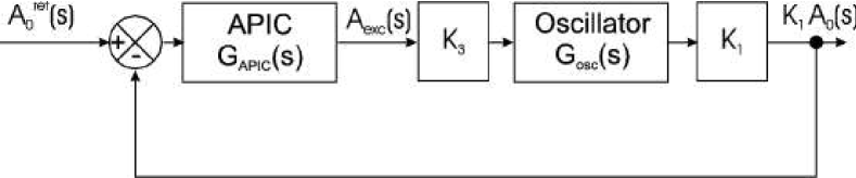
Figure 13: Simplified scheme of the closed loop for the characterization of the response time of the APIC.

The problem consists in analyzing the dynamics of the oscillator the amplitude of which is controlled by a proportional-integral controller. For that purpose, all the components are assumed to be linear. No interaction occurs between the oscillator and the surface. The contributions of the RMS-to-DC and of the band pass filter are neglected. The system under investigation is given in figure 13.

VII.2.1 Transfer function of the closed loop

We start from the set of equations 35 wherein the phase is assumed to be constant and fixed to $\varphi(t)\rightarrow\varphi=-\pi/2$. This assumption is argued by the PLL behavior which maintains the phase almost constant, even when the interaction occurs (cf. fig. 3(b)). The assumption implies : $\omega=\omega_{0}$, $\dot{\varphi}(t)=\ddot{\varphi}(t)=0$ and obviously, we only focus at changes occurring in the resonance amplitude $A(t)=A_{0}(t)$. The set of equations 35 is then equivalent to :

$$\left\{\begin{array}[]{ll}\beta=\gamma\\ \alpha=0\end{array}\right.$$ (47)

Keeping $\beta=\gamma$ yields to :

$$\dot{A}_{0}(t)=\frac{\omega_{0}}{2}\left\{K_{3}A_{exc}-\frac{A_{0}(t)}{Q}\right\}$$ (48)

The transfer function of the block standing for the oscillator can thus be written :

$$G_{osc}(s)=\frac{K_{1}A_{0}(s)}{A_{exc}(s)}=K_{1}K_{3}\frac{b}{s+a}$$ (49)

where :

$$\left\{\begin{array}[]{ll}b=\frac{\omega_{0}}{2}\\ a=\frac{\omega_{0}}{2Q}\end{array}\right.$$ (50)

The transfer function of the APIC being $G_{APIC}(s)=K_{p}^{\text{ac}}+K_{i}^{\text{ac}}/s$, the transfer function of the closed loop $G_{cl}(s)=K_{1}A_{0}(s)/A_{0}^{ref}(s)$ can now be calculated :

$$G_{cl}(s)=\frac{b\tilde{K}_{p}^{\text{ac}}s+b\tilde{K}_{i}^{\text{ac}}}{s^{2}+(a+b\tilde{K}_{p}^{\text{ac}})s+b\tilde{K}_{i}^{\text{ac}}},$$ (51)

with :

$$\left\{\begin{array}[]{ll}\tilde{K}_{p}^{\text{ac}}=K_{1}K_{3}K_{p}^{\text{ac}}\\ \tilde{K}_{i}^{\text{ac}}=K_{1}K_{3}K_{i}^{\text{ac}}\end{array}\right.$$ (52)

The proportional and integral gains are scaled by the transfer functions of the piezoelectric actuator and of the photodiodes, $K_{3}$ and $K_{1}$, respectively.

VII.2.2 Analogy

Equation 51 has two poles :

$$s_{1,2}=-c\pm\sqrt{c^{2}-b\tilde{K}_{i}^{\text{ac}}},$$ (53)

where $c$ is the parameter given in equation 33, which can also be written :

$$c=\frac{a+b\tilde{K}_{p}^{\text{ac}}}{2}$$ (54)

Equation 51 is thus almost analog to a standard $2^{nd}$ order system, the canonical form of which can be written :

$$G(s)=\frac{\omega_{n}^{2}}{s^{2}+2\zeta\omega_{n}s+\omega_{n}^{2}},$$ (55)

where $\omega_{n}$ and $\zeta$ are the characteristic frequency and damping factor of the system, respectively. Thus :

$$\zeta=\frac{c}{\sqrt{b\tilde{K}_{i}^{\text{ac}}}}$$ (56)

Now, it’s well known that the position of $\zeta$ with respect to 1 defines the overall behavior of the system :

$$\left\{\begin{array}[]{lll}\text{Undercritically damped regime }\Rightarrow\zeta<1\Leftrightarrow c<\sqrt{b\tilde{K}_{i}^{\text{ac}}}\\ \text{Critically damped regime }\Rightarrow\zeta=1\Leftrightarrow c=\sqrt{b\tilde{K}_{i}^{\text{ac}}}\\ \text{Overcritically damped regime }\Rightarrow\zeta>1\Leftrightarrow c>\sqrt{b\tilde{K}_{i}^{\text{ac}}}\end{array}\right.$$ (57)

VII.2.3 Analysis to a step response

To assess how fast the controller reacts, we investigate the response of the controller to a step in amplitude upon it is in the over-, under- or critically damped regime. Let’s assume a step of amplitude $A_{s}$, the corresponding transfer function is $G_{s}(s)=A_{s}/s$ and the transfer function of the closed loop system to which the step is applied is therefore $G_{cls}(s)=G_{s}(s)\times G_{cl}(s)$, that is :

$$G_{cls}(s)=\frac{A_{s}b\tilde{K}_{p}^{\text{ac}}}{\left(s+c\right)^{2}-c^{2}+b\tilde{K}_{i}^{\text{ac}}}+\frac{A_{s}b\tilde{K}_{i}^{\text{ac}}}{\left(s+c\right)^{2}-c^{2}+b\tilde{K}_{i}^{\text{ac}}}\times\frac{1}{s}$$ (58)

The time-dependent solutions $g_{cls}(t)=\mathcal{L}^{-1}\{G_{cls}(s)\}$ are :

• Overcritically damped regime : $c>\sqrt{b\tilde{K}_{i}^{\text{ac}}}$
  

  $$g_{cls}(t)=A_{s}\left\{1+\varsigma_{-}e^{-(c+\xi)t}-\varsigma_{+}e^{-(c-\xi)t}\right\}$$ (59)

  with $\varsigma_{\pm}=(c\pm\xi-b\tilde{K}_{p}^{\text{ac}})/2\xi$ and $\xi=\sqrt{c^{2}-b\tilde{K}_{i}^{\text{ac}}}$.

• Critically damped regime : $c=\sqrt{b\tilde{K}_{i}^{\text{ac}}}$

  $$g_{cls}(t)=A_{s}\left\{1-e^{-ct}+\left[b\tilde{K}_{p}^{\text{ac}}-c\right]te^{-ct}\right\}$$ (60)

• Undercritically damped regime : $c<\sqrt{b\tilde{K}_{i}^{\text{ac}}}$

  $$g_{cls}(t)=A_{s}\left\{1-e^{-ct}\times\left[\cos\left(\xi^{\prime}t\right)+\frac{c-b\tilde{K}_{p}^{\text{ac}}}{\xi^{\prime}}\sin\left(\xi^{\prime}t\right)\right]\right\}$$ (61)

  with $\xi^{\prime}=\sqrt{b\tilde{K}_{i}^{\text{ac}}-c^{2}}$.

VII.2.4 Summary

The transition from the over to the under critically damped regime is thus controlled by the parameter $c$, that is the proportional gain, and occurs when the condition $c=\sqrt{b\tilde{K}_{i}^{\text{ac}}}$ is fulfilled. In the critically damped regime, the relationship between the two gains is :

$$\tilde{K}_{i}^{\text{ac}}=\frac{\omega_{0}}{8}\left(\frac{1}{Q}+\tilde{K}_{p}^{\text{ac}}\right)^{2}$$ (62)

The time constant of the system can be extracted upon the regime and the time scale that are considered. For short time scales, the response time of the controller is typically $1/c$ in the critically damped regime and $t_{\text{resp}}=1/(c+\sqrt{c^{2}-b\tilde{K}_{i}^{ac}})$ in the overcritically damped regime (cf. equ.59), which is given in equation 32. Figure 7 shows that the response times of the real system and of the simulated machine reasonably match $t_{\text{resp}}$ while the RMS-to-DC converter has a negligible influence on the system dynamics.

Figures

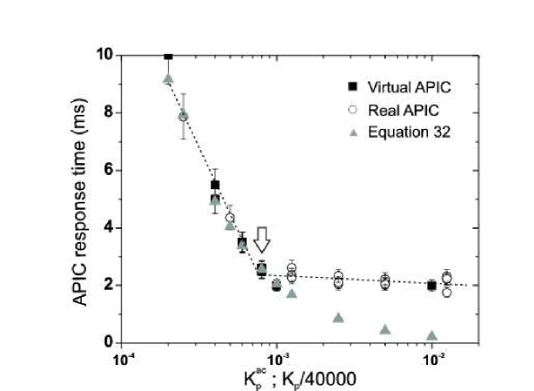
Figure 7: Response time of the APIC vs. $K_{p}^{\text{ac}}$ of the simulated setup and the rescaled $K_{p}$ gain of the real controller. The best agreement between the curves is obtained with $K_{p}/40000$. The two curves match with a reasonable agreement and exhibit two domains : first the response time decreases when increasing $K_{p}^{\text{ac}}$ and then a saturation is reached corresponding to $t_{\text{resp}}\simeq 2$ ms. The dotted line is given as guide eyes. Such an analysis can be performed assuming that the step response is governed by a single time constant, thus restricting the analysis to curves which exhibit an almost critically damped behavior (cf. text). The triangles depict the trace of the function $t_{\text{resp}}$ (equ. 32) with $f_{0}=157514.6$ Hz, $Q=36000$, $K_{1}=0.1$ V.nm^-1 and $K_{3}=1/K_{1}$ nm.V^-1. The arrow denotes the value of the gain used to perform the scan lines (cf. section V). Beyond $K_{p}^{\text{ac}}=10^{-3}$, a noticeable discrepancy between the theoretical model and the experiments is observed which might be due to the contribution of the RMS-to-DC converter.

Figure 10: Calculated cross-section of a sinusoidally corrugated surface for various PLL gains, namely $K_{0}K_{d}=100$ rad.s^-1 (continuous black line), $1000$ rad.s^-1 (continuous grey line) and $5000$ rad.s^-1 (dotted black line). The scan lines have been initiated from the approach curve shown on fig.3 by $\Delta f$ regulation using $\Delta f_{\text{set}}=-60$ Hz. The lateral scan speed is $7$ nm.s^-1 and the section consists of 256 samples. $K_{p}^{\text{dc}}=2\times 10^{-3}$ nm.Hz^-1 and $K_{i}^{\text{dc}}=2$ nm.Hz^-1.s^-1, corresponding to a critically damped response of the controller to a frequency step of $-1$ Hz. (a)- Topography. (b)- Frequency shift. (c)- Phase lag $\varphi$. (d)- Amplitude $A_{\text{rms}}/K_{1}$ and (e)- relative damping. No noticeable effect is revealed on the topography. The apparent dissipation remains below the thermal noise (cf. section IV), except if the PLL is slow ($K_{0}K_{d}=100$ rad.s^-1, $12\%$).