The dynamics of transition to turbulence in plane Couette flow

Abstract

In plane Couette flow, the incompressible fluid between two plane parallel walls is driven by the motion of those walls. The laminar solution, in which the streamwise velocity varies linearly in the wall-normal direction, is known to be linearly stable at all Reynolds numbers ($Re$). Yet, in both experiments and computations, turbulence is observed for $Re\gtrsim 360$.

In this article, we show that for certain threshold perturbations of the laminar flow, the flow approaches either steady or traveling wave solutions. These solutions exhibit some aspects of turbulence but are not fully turbulent even at $Re=4000$. However, these solutions are linearly unstable and flows that evolve along their unstable directions become fully turbulent. The solution approached by a threshold perturbation could depend upon the nature of the perturbation. Surprisingly, the positive eigenvalue that corresponds to one family of solutions decreases in magnitude with increasing $Re$, with the rate of decrease given by $Re^{\alpha}$ with $\alpha\approx-0.46$.

1 Introduction

1.1 Transition to turbulence

The classical problem of transition to turbulence in fluids has not been fully solved in spite of attempts spread over more than a century. Transition to turbulence manifests itself in a simple and compelling way in experiments. For instance, in the pipe flow experiment of Reynolds (see [1]), a dye injected at the mouth of the pipe extended in “a beautiful straight line through the tube” at low velocities or low Reynolds numbers ($Re$). The line would shift about at higher velocities, and at yet higher velocities the color band would mix up with the surrounding fluid all at once at some point down the tube.

A wealth of evidence shows that the incompressible Navier-Stokes equation gives a good description of fluid turbulence. Therefore one ought to be able to understand the transition to turbulence using solutions of the Navier-Stokes equation. However, the nature of the solutions of the Navier-Stokes equation is poorly understood. Thus the problem of transition to turbulence is fascinating both physically and mathematically.

The focus of this paper is on plane Couette flow. In plane Couette flow, the fluid is driven by two plane parallel walls. If the fluid is driven hard enough, the flow becomes turbulent. Such wall driven turbulence occurs in many practical situations such as near the surface of moving vehicles and is technologically important.

The two parallel walls are assumed to be at $y=\pm 1$. The walls move in the $x$ or streamwise direction with velocities equal to $\pm 1$. The $z$ direction is called the spanwise direction. The Reynolds number is a dimensionless constant obtained as $Re=UL/\nu$, where $U$ is half the difference of the wall velocities, $L$ is half the separation between the walls, and $\nu$ is the viscosity of the fluid. The velocity of the fluid is denoted by ${\bf u}=(u,v,w)$, where $u,v,w$ are the streamwise, wall-normal, and spanwise components.

For the laminar solution, $v=w=0$ and $u=y$. The laminar solution is linearly stable for all $Re$. As shown by Kreiss et al.​​ [7], perturbations to the laminar solution that are bounded in amplitude by $O(Re^{-21/4})$ decay back to the laminar solution. However, in experiments and in computations, turbulent spots are observed around $Re=360$ [2]. The transition to turbulence in such experiments must surely be because of the finite amplitude of the disturbances. By a threshold disturbance, we refer to a disturbance that would lead to transition if it were slightly amplified but which would relaminarize if slightly attenuated. The concept of the threshold for transition to turbulence was introduced by Trefethen and others [16]. The amplitude of the threshold disturbance depends upon the type of the disturbance. It is believed to scale with $Re$ at a rate given by $Re^{\alpha}$ for some $\alpha<=-1$.

Figure 1: Schematic sketch of the dynamical picture of transition to turbulence that is developed in this paper. The solid oval stands for the laminar solution, and the empty oval stands for a steady or traveling wave solution.

Our main purpose is to explain how certain finite amplitude disturbances of the laminar solution lead to turbulence. The dynamical picture that will be developed in this paper is illustrated in Figure 1. Historically, the laminar solution itself has been the focus of attempts to understand mechanisms for transition. Our focus however will be on a different solution that is represented as an empty oval in Figure 1.

Solutions that could correspond to the empty oval in Figure 1 will be called lower-branch solutions [11, 19]. A solution at a certain value of $Re$ can be continued by increasing a carefully chosen parameter. When this parameter is increased, $Re$ first decreases and begins to increase after a bifurcation point and we end up with an “upper branch solution” at the original value of $Re$. The fact that a continuation procedure can lead to an upper-branch solution appears to have no significance for the dynamics at a fixed value of $Re$, however

Depending upon the type of disturbance, the lower-branch solution could either be a steady solution or a traveling wave. Those solutions are not laminar in nature. Neither are they fully turbulent even at high $Re$. Unlike the laminar solution, these solutions are linearly unstable. The lower-branch solutions remain at an $O(1)$ distance from the laminar solution, while the threshold amplitudes decrease with $Re$ as indicated already. Therefore the threshold disturbances are too tiny to perturb the laminar solution directly onto a lower-branch solution. We will show, however, that some threshold disturbances perturb the laminar solution to a point on the stable manifold of a lower-branch solution (point $P$ in Figure 1). A slightly larger disturbance brings the flow close to the lower-branch solution, after which the flow follows a branch of its unstable manifold and becomes fully turbulent.

For certain types of disturbances, the perturbed laminar solution does not approach a lower branch solution. Thus the dynamical picture of Figure 1 is not valid for those disturbances. Instead it flows towards an edge state [15]. We give a brief discussion of the nature of the edge states in Section 4.

1.2 Connections to earlier research

The dynamical picture presented in Figure 1 is related directly and indirectly to much earlier research. Basic results from hydrodynamic stability show that some eigenmodes that correspond to the least stable eigenvalue of the linearization around the laminar solution do not depend upon the spanwise or $z$ direction. This may lead one to expect that disturbances that trigger transition to turbulence are $2$-dimensional. That expectation is not correct, however. As shown by Orszag and Kells [13], spanwise variation is an essential feature of disturbances that trigger transition to turbulence. Accordingly, all the disturbances considered in this paper are $3$-dimensional.

Kreiss et al.​​ [7] and Lundbladh et al.​​ [9] investigated disturbances that are non-normal pseudomodes of the linearization of the laminar solution. Since the laminar solution is linearly stable, a slight perturbation along an eigenmode will simply decay back to the laminar solution at a predictable rate. The pseudomodes are chosen to maximize transient growth of the solution of the linearized equation, which is a consequence of the non-normality of the linearization. Such disturbances lead to transition with quite small amplitudes and will be considered again in this paper. It must be noted, however, that any consideration based on the linearization alone can only be valid in a small region around the laminar solution. The dynamics of transition to turbulence, as sketched in Figure 1, involves an approach towards a lower-branch solution that lies at an $O(1)$ distance from the laminar solution. It is therefore necessary to work with the fully nonlinear Navier-Stokes equation to explicate the dynamics of transition to turbulence.

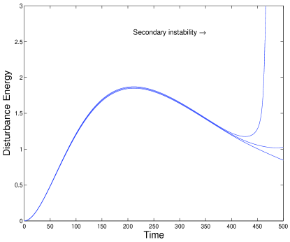
Figure 2: The plot above shows the secondary instability in a transition computation at $Re=2000$.

Figure 2 shows the variation of the disturbance energy with time for a disturbance that leads to transition. We observe that the disturbance energy increases smoothly initially and is then followed by a spike. The spike is in turn followed by turbulence. The spike corresponds to a secondary instability, as noted by Kreiss et al.​​ [7]. In fact, the so-called secondary instability is just the linear instability of a lower-branch solution as will become clear.

Partly motivated by the secondary instability, there was a search for nonlinear steady solutions related to transition as reviewed in [3]. Early success in this effort was due to Nagata [11, 12] who computed steady solutions of plane Couette flow in the interval $125\leq Re\leq 300$. Waleffe [18, 19, 20] introduced a more flexible method for computing such solutions, and like Nagata, argued that such solutions could be related to transition to turbulence. The numerical method we use was introduced in [17]. It uses a combination of Krylov space methods and the locally optimally constrained hook step to achieve far better resolution as show by [4], [17], [21], and this paper.

The computations in [7, 9] imply that threshold amplitudes scale as $Re^{\alpha}$ for $\alpha<-1$. The value of $\alpha$ appears to depend upon the type of perturbation. Our focus is not on determining the scaling of the threshold amplitudes. Nevertheless, we will discuss numerical difficulties that beset determination of threshold amplitudes.

Measuring threshold amplitudes poses experimental challenges as well and it is not always clear from experiments if the thresholds have a simple power scaling with $Re$. One difficulty is that the turbulent states can be short lived. Schmiegel and Eckhardt [14] have connected the lifetime of turbulence to the possibility that turbulent dynamics in the transition regime is characterized by a chaotic saddle and not a chaotic attractor.

1.3 Connections to recent research

Wang et al.​​ [21] have taken steps towards an asymptotic theory of the lower branch solutions and carried their computation beyond $Re=50,000$. They connect the asymptotics to scalings of the threshold for transition to turbulence. The lower branch states occur as solutions to equations that use periodic boundary conditions. Because such boundary conditions cannot be realized in laboratory setups, the solutions are best thought of as waves. Thus it is pertinent to consider their stability with respect to subharmonic disturbances as in [21]. That paper also suggests that lower branch solutions might be of use for control. A somewhat different suggestion related to control can be found in [5].

Not all disturbances follow the dynamical picture of Figure 1 as already noted. For the third type of disturbance considered in Section 4, the laminar solution perturbed by the threshold disturbance evolves towards a state that looks almost like an invariant object of the underlying differential equation. Those objects have been termed edge states by Schnieder et al.​​ [15]. Lagha et al.​​ [8] make the important point that the dynamical picture of Figure 1 can be valid for typical disturbances only if the lower-branch solution has a single unstable eigenvalue.

Near the threshold for the third type of disturbance, it appears as if the disturbed state evolves and approaches a traveling wave. Indeed, a crude or under-resolved computation could easily mistake that appearance for a true solution. When we attempted to refine that near-solution using the numerical method reviewed in Section 3, the numerical method converged to a traveling wave solution. However, that traveling wave has two unstable eigenvalues and the flow near the threshold does not come as close to that traveling wave as the dynamical picture of Figure 1 would require. The disturbed state appears to evolve into an edge state.

Visualizing the dynamics in state space is fundamental to the approach to transition to turbulence sketched in this paper and in the articles discussed above. Yet there has so far been no way to obtain revealing visualizations of state space dynamics. Gibson et al.​​ [4] have recently produced revealing visualizations of the state space of turbulent flows. For instance, one of their figures shows a messy-looking turbulent trajectory cleanly trapped by the unstable manifolds of certain equilibrium solutions. Such visualizations might prove useful to both computational and experimental investigations of transition to turbulence

Section 2 reviews some basic aspects of plane Couette flow. The numerical method used to flesh out the dynamical picture of Figure 1 is given in Section 3. In Section 4, we consider three different types of disturbances. The lower-branch solutions (empty oval of Figure 1) that correspond to the first two types are steady solutions. For a given $Re$, the solutions that correspond to these two types are identical modulo certain symmetries of plane Couette flow. In Section 5, we consider some qualitative aspects of the solutions reported in Section 4. A surprising finding is that these these solutions are less unstable for larger $Re$. The top eigenvalue of these solutions is real and positive. For one family of solutions, the top eigenvalue appears to decrease at the rate $Re^{\alpha}$ for $\alpha\approx-0.46$.

In the concluding Section 6, we give additional context for this paper from two points of view. The first point of view is mainly computational and has to do with reduced dimension methods. In this paper, we have taken care to use adequate spatial resolution to ensure that the computed solutions are true solutions of the Navier-Stokes equation. We recognize, however, that resolving all scales may prove computationally infeasible in some practical situations. We argue that transition to turbulence computations can be useful in gaging the possibilities and limitations of methods that do not resolve all scales. Secondly, we briefly discuss the connection of transition computations with transition experiments.

2 Some aspects of plane Couette flow

The Navier-Stokes equation $\partial{\bf u}/\partial t+({\bf u}.\nabla){\bf u}=-(1/\rho)\nabla p+(1/Re)\triangle{\bf u}$ describes the motion of incompressible fluids. The velocity field ${\bf u}$ satisfies the incompressible constraint $\nabla.{\bf u}=0$. For plane Couette flow the boundary conditions are ${\bf u}=(\pm 1,0,0)$ at the walls, which are at $y=\pm 1$. To render the computational domain finite, we impose periodic boundary conditions in the $x$ and $z$ directions, with periods $2\pi\Lambda_{x}$ and $2\pi\Lambda_{z}$, respectively. To enable comparison with [9], we use $\Lambda_{x}=1.0$ and $\Lambda_{z}=0.5$ throughout this paper.

Certain basic quantities are useful for forming a general idea of the nature of a velocity field of plane Couette flow. The first of these is the rate of energy dissipation per unit volume for plane Couette flow, which is given by

$$D=\frac{1}{8\pi^{2}\Lambda_{x}\Lambda_{z}}\int_{0}^{2\pi\Lambda_{z}}\int_{-1}^{+1}\int_{0}^{2\pi\Lambda_{x}}\left|\nabla u\right|^{2}+\left|\nabla v\right|^{2}+\left|\nabla w\right|^{2}\>dx\,dy\,dz.$$ (2.1)

The rate of energy input per unit volume is given by

$$I=\frac{1}{8\pi^{2}\Lambda_{x}\Lambda_{z}}\int_{0}^{2\pi\Lambda_{x}}\int_{0}^{2\pi\Lambda_{z}}\frac{\partial u}{\partial y}\Bigl{\lvert}_{y=1}+\frac{\partial u}{\partial y}\Bigl{\lvert}_{y=-1}\>dx\,dz.$$ (2.2)

For the laminar solution $(u,v,w)=(y,0,0)$, both $D$ and $I$ are normalized to evaluate to $1$. Expressions such as (2.1) and (2.2) are derived using formal manipulations. The derivations would be mathematically valid if the velocity field ${\bf u}$ were assumed to be sufficiently smooth. Although such smoothness properties of solutions of the Navier-Stokes are yet to be proved, numerical solutions possess the requisite smoothness. Even solutions in the turbulent regime appear to be real analytic in the time and space variables, which is why spectral methods have been so successful in turbulence computations.

In the long run, on physical grounds, we expect the time averages of $D$ and $I$ to be equal because the energy dissipated through viscosity must be input at the walls. For steady solutions and traveling waves, the values of $D$ and $I$ must be equal.

Another useful quantity is the disturbance energy. The disturbance energy of $(u,v,w)$ is obtained by integrating $(u-y)^{2}+v^{2}+w^{2}$ over the computational box. This quantity has already been used in Figure 2. The disturbance energy is a measure of the distance from the laminar solution.

Two discrete symmetries of the Navier-Stokes equation for plane Couette flow will enter the discussion later. The shift-reflection transformation of the velocity field is given by

$$S_{1}{\bf u}=\begin{pmatrix}u\\ v\\ -w\end{pmatrix}\Biggl{(}x+\pi\Lambda_{x},y,-z\Biggr{)},$$ (2.3)

and the shift-rotation transformation of the velocity field is given by

$$S_{2}{\bf u}=\begin{pmatrix}-u\\ -v\\ w\end{pmatrix}\Biggl{(}-x+\pi\Lambda_{x},-y,z+\pi\Lambda_{z}\Biggr{)}.$$ (2.4)

Plane Couette flow is unchanged under both these transformations. Thus if a single velocity field along a trajectory of plane Couette flow satisfies either symmetry, all points along the trajectory must have the same symmetry. However, velocity fields that lie on the stable and unstable manifolds of symmetric periodic or relative periodic solutions need not be symmetric.

3 Numerical method

The Navier-Stokes equation in the standard form given in Section 2 cannot be viewed as a dynamical system because the velocity field ${\bf u}$ must satisfy the incompressibility condition and because there is no equation for evolving the pressure $p$. It can be recast as a dynamical system, however, by using the $y$ components of ${\bf u}$ and $\nabla\times{\bf u}$, which is the vorticity field. If the resulting system is discretized in space using $M+1$ Chebyshev points in the $y$ direction, and $2L$ and $2N$ Fourier points in the $x$ and $z$ directions, respectively, the number of degrees of freedom of the spatially discretized system is given by

$$2(M-1)+(2M-4)((2N-1)(2L-1)-1)$$ (3.1)

as shown in [17]. We do not use a truncation strategy to discard modes and we employ dealiasing in the directions parallel to the wall.

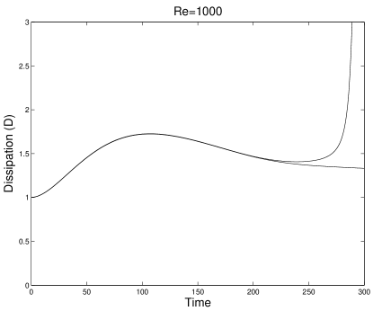
Figure 3: The plot above shows the variation of $D$ defined by (2.1) for a disturbance slightly above the threshold and for a disturbance slightly below the threshold.

Given a form of the disturbance $P$, the threshold for transition is obtained by integrating the disturbed velocity $(y,0,0)+\epsilon P$ in time for different $\epsilon$ [7]. If $\epsilon$ is greater than the threshold value, the flow will spike and become turbulent as evident from Figures 2 and 3. If $\epsilon$ is below the threshold value, the flow will relaminarize. As indicated by Figures 2 and 3, we may graph either disturbance energy or $D$ to examine a value of $\epsilon$. We may also graph $I$, which is defined by (2.2), against time.

The accurate determination of thresholds is beset by numerical difficulties. To begin with, suppose that we are able to integrate the Navier-Stokes equation for plane Couette flow exactly. Then as implied by the dynamical picture in Figure 1, a disturbance of the laminar solution that is on the threshold will fall into a lower-branch solution, and it will take infinite time to do so. However, computations for determining the threshold, such as that shown in Figure 2, can only be over a finite interval of time. Thus the finiteness of the time of integration is a source of error in determining thresholds. Two other sources of error are spatial discretization and time discretization.

An accurate determination of the threshold will need to estimate and balance these three sources of error carefully. In our computations, we determine the thresholds with only about $2$ digits of accuracy. That modest level of accuracy is sufficient for our purposes. In Tables 1 and 3, the thresholds are reported using disturbance energy per unit volume.

Once the threshold has been determined, we need to compute a steady solution or a traveling wave to complete the dynamical picture of Figure 1. The initial guess for that lower-branch solution is produced by perturbing the laminar solution by adding the numerically determined threshold disturbance and integrating the perturbed point over the time interval used for determining the threshold (this time interval is $500$ in Figure 2 and $300$ in Figure 3).

That initial guess is fed into the method described in [17] to find a lower-branch solution with good numerical accuracy. That method finds solutions by solving Newton’s equations, but the equations are set up and solved in a non-standard way. Suppose that the spatially discretized equation for plane Couette flow is written as $\dot{x}=f(x)$, where the dimension of $x$ is given by (3.1). To find a steady solution, for instance, it is natural to solve $f(x)=0$ after supplementing that equation by some conditions that correspond to the symmetries (2.3) and (2.4). However that is not the way we proceed. We solve for a fixed point of the time $t$ map $x(t;x_{0})$, for a fixed value of $t$, after accounting for the symmetries. The Newton equations are solved using GMRES. The method does not always compute the full Newton step, however. Instead, the method finds the ideal trust region step within a Krylov subspace as described in [17].

This method can easily handle more than $10^{5}$ degrees of freedom, and thus makes it possible to carry out calculations with good spatial resolution. The reason for setting up the Newton equations in the peculiar way described in the previous paragraph has to do with the convergence properties of GMRES. The matrix that arises in solving the Newton equations approximately has the form $I-\partial x(t;x_{0})/\partial x_{0}$, where $I$ is the identity. Because of viscous damping of high wavenumbers, many of the eigenvalues of that matrix will be close to $1$, thus facilitating convergence of GMRES. We may expect the convergence to deteriorate as $Re$ increases, because viscous damping of high wavenumbers is no longer so pronounced, and that is indeed the case. Nevertheless, we were able to go up to $Re=4000$, and we believe that even higher values of $Re$ can be reached.

4 Disturbances of the laminar solution and transition to turbulence

In this section, we consider three types of disturbances and determine the threshold amplitudes for various values of $Re$. To complete the dynamical picture of Figure 1, we determine for the first two types the steady solution or traveling wave that corresponds to the empty oval of that figure using the numerical method of the previous section.

4.1 Rolls with unsymmetric noise

Label	$Re$	$D$/$I$	$\lambda_{max}$	$Re_{\tau}$	$T$	threshold
$B1$	$500$	$1.3920$	$.04326$	$53$	$150$	$2.46e-4$
$B2$	$1000$	$1.3486$	$.03294$	$73$	$300$	$5.73e-5$
$B3$	$2000$	$1.3285$	$.02413$	$103$	$500$	$1.36e-5$
$B4$	$4000$	$1.3210$	$.01732$	$145$	$1000$	$3.30e-6$

Table 1: Data for disturbances of the form (4.1) with unsymmetric noise and for steady solutions that correspond to the empty oval in Figure 1. The steady solutions are labeled $B1$ through $B4$. $D$ and $I$, which are defined by (2.1) and (2.2), correspond to those steady solutions. The next two columns give the eigenvalue with the maximum real part and the frictional Reynolds number for those solutions. $T$ is the time interval used to determine the threshold disturbance and the threshold is reported using disturbance energy per unit volume.

We follow [7] and consider the disturbance,

$$(u,v,w)=\epsilon(0,\psi_{z},-\psi_{y}),$$ (4.1)

where $\psi=(1-y^{2})^{2}\sin(z/\Lambda_{z})$. This disturbance is unchanged by both $S_{1}$, which was defined by (2.3), and by $S_{2}$, which was defined by (2.4). A disturbance of the laminar solution ${\bf u}=(y,0,0)$ of the form (4.1) never leads to transition to turbulence. It is necessary to add some more terms to the disturbance to make the velocity field depend upon the $x$ direction.

To introduce dependence on $x$, we add modes of the Stokes problem. One can get an eigenvalue problem for $\hat{v}(y)$, where $v=\hat{v}(y)\exp(\iota lx/\Lambda_{x}+\iota nz/\Lambda_{z})\exp(\sigma t)$, or for $\hat{\eta}(y)$, where $\eta=\hat{\eta}(y)\exp(\iota lx/\Lambda_{x}+\iota nz/\Lambda_{z})\exp(\sigma t)$. Here $\eta$ is the wall-normal component of the vorticity field. For a $v$ mode, $\eta=0$, and vice versa. For a given mode, the velocity field is recovered using the divergence free condition. The velocity fields of modes with different $(l,n)$ are obviously orthogonal. A calculation shows that the velocity fields for the $v$ and $\eta$ modes with the same $(l,n)$ are also orthogonal. For a given $(l,n)$, we pick the $v$ and $\eta$ modes with the least stable $\sigma$.

To the disturbance (4.1), we added both $v$ and $\eta$ modes for $(l,n)$ with $-3\leq l\leq 3$ and $-7\leq n\leq 7$. Together the added modes can be called noise. The energy of the noise was equal to $1\%$ of the energy of (4.1). This energy was equally distributed over the various orthogonal modes. Following [7], we chose random phases for the modes. The threshold can depend upon the choice of phase. Therefore, for accurate determination of thresholds it is better to use non-random phases.

After adding modes of this form to (4.1), the resulting disturbance in unchanged by neither $S_{1}$ nor $S_{2}$. Therefore the disturbance is unsymmetric. Table 1 reports data from computations carried out using such an unsymmetric disturbance. The thresholds in that table give the energy of (4.1) and do not include the energy within the noise terms. The lower-branch solutions $B1$ through $B4$ correspond to the empty oval in Figure 1. Each of these solutions appears to have a single unstable eigenvalue. We determined the most unstable eigenvalues using simultaneous iteration and the time $t$ map of the Navier-Stokes equation, as in Section 3, with $t=8$. All the solutions seem to have just one unstable eigenvalue. That eigenvalue is real. Surprisingly, it decreases with $Re$ at the rate $Re^{\alpha}$, where $\alpha\approx-0.46$. Thus the lower-branch solutions become less and less unstable with increasing $Re$.

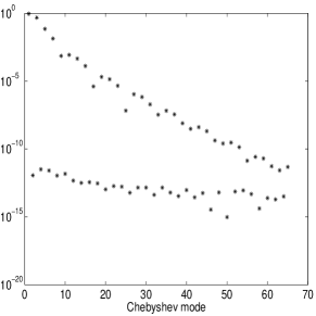
Figure 4: The plots above graph the energy in the solution $B4$ of Table 1 against streamwise wavenumber, spanwise wavenumber, and Chebyshev mode.

All our computations used $(2L,M+1,2N)=(24,65,32)$. By (3.1), the number of degrees of freedom in the computation for finding the lower-branch solutions is $88414$. As shown by Figure 4, that much resolution was entirely adequate. The solutions $B1$ through $B4$ were computed with at least $5$ digits of accuracy.

4.2 Rolls with symmetric noise

Label	$Re$	$s_{x}$	$s_{z}$	Threshold
$C1$	$500$	$1.5600$	$.0016$	$2.97e-4$
$C2$	$1000$	$6.1093$	$.0012$	$5.72e-5$
$C3$	$2000$	$0.5075$	$.0018$	$1.40e-5$
$C4$	$4000$	$2.8719$	$.0013$	$3.28e-6$

Table 2: Data for disturbances of the form (4.1) with symmetric noise and steady solutions that correspond to the empty oval in Figure 1. The solutions $Cn$ are connected to the solutions $Bn$ of Table 1 as follows: $Cn(x+s_{x},y,z+s_{z})=Bn$.

It has been suggested that one purpose of adding the noise to (4.1) is to break symmetries and that a symmetric disturbance would lead to drastically increased thresholds [7]. To investigate that matter, we symmetrized the disturbances used to generate Table 1. More specifically, if ${\bf u}$ is a disturbed velocity field, we replaced it by $({\bf u}+S_{1}{\bf u}+S_{2}{\bf u}+S_{1}S_{2}{\bf u})/4$ which is unchanged by both $S_{1}$ and $S_{2}$. A comparison of Tables 1 and 2 shows that the thresholds are in fact not elevated. Thus we conclude that the purpose of adding the noise is not to break the symmetry but to introduce dependence on the $x$ direction. The lower-branch solutions that correspond to such symmetric disturbances are labeled $C1$ through $C4$ in Table 2.

The solutions $C1$ though $C4$ are just translations of the solutions $B1$ through $B4$ as indicated in Table 2. If the thresholds were determined exactly, the disturbances of Tables 1 and 2 would come arbitrarily close to the corresponding solution in the infinite time limit. Each threshold in those tables was determined inexactly using a finite time interval, and we verified that the disturbed states evolve and come within $2\%$ of the corresponding lower-branch solution. Thus there can be little doubt about the role of these lower-branch solutions in the transition to turbulence. The $C$ family of solutions is the same as the lower-branch family of [20].

Given that the solutions $C1$ through $C4$ are just translations of the solutions $B1$ through $B4$, it is tempting to think that all threshold disturbances, say at $Re=4000$, might evolve and approach a translate of a single solution such as $C4$. That is not correct, however, as we will now show.

4.3 Superposed Orr-Sommerfeld modes

Label	$Re$	$D/I$	$\lambda_{max}$	$Re_{\tau}$	$c_{x}$	$c_{z}$	$T$	Threshold
$D1$	$500$	$1.2863$	$.0464$	$51$	$.3051$	$0$	$100$	$8.4e-3$
$D2$	$1000$	$1.2522$	$.0379$	$72$	$.2666$	$0$	$200$	$1.6e-3$

Table 3: Data for disturbances obtained by superposing Orr-Sommerfeld modes and for the corresponding traveling waves labeled $D1$ and $D2$. $c_{x}$ and $c_{z}$ give the wave speeds in the $x$ and $z$ directions. The other columns are as in Table 1.

The disturbances for Table 3 were obtained by superposing Orr-Sommerfeld modes as in [13]. An Orr-Sommerfeld mode is of the form $(u,v,w)=(\hat{u}(y),\hat{v}(y),\hat{w}(y))\exp(\iota lx/\Lambda_{x}+\iota nz/\Lambda_{z})\exp(\sigma t)$. We use Orr-Sommerfeld modes with $(l,n)=\pm(1,0)$ and $(l,n)=\pm(1,1)$. The phases of the Orr-Sommerfeld modes were chosen to make $\hat{v}(0)$ real. The disturbance energy was equally distributed across the modes. For given $(l,n)$, we chose the least stable mode and symmetrized it as in Equation (3.2) of [13]. Note that the disturbance depends on both the $x$ and $z$ directions.

The solutions obtained by following the numerical method of Section 3 were traveling waves in this case. The wave speeds for both $D1$ and $D2$ in Table 3 are nonzero in the $x$ direction. These traveling waves are unsymmetric and they do not become symmetric even after translations in the $x$ and $z$ directions.

The thresholds for this third type of disturbance are reported in Table 3. Close to the threshold, the flow appears to approach a traveling wave. After a diligent computation, we feel sure that there is no true traveling wave solution or relative periodic solution to complete the dynamical picture of Figure 1. The flow near the threshold evolves and comes within $10\%$ of $D1$ or $D2$ but no closer. It appears to approach an edge state.

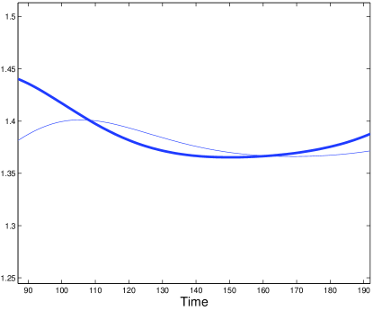
Figure 5: The thick line is a plot of $D$ defined by (2.1) and the thin line is a plot of $I$ defined by (2.2). The disturbance used to get the plots was a superposition of Orr-Sommerfeld modes at $Re=500$.

Figure 5 shows plots of the rates of energy input and energy dissipation near an edge state. In that figure, the disturbance is very close to the threshold and the time axis is chosen to correspond to an edge state. Note that the dissipation sags below energy input and then rises above it. Therefore, we do not expect a traveling wave or an equilibrium solution near the edge state. The second crossing of the two curves is below the first. In addition, both the curves spike and transition to turbulence soon after they cross. Therefore, a periodic or relative periodic solution is unlikely to be found near the edge state.

In pipe flow transition computations, we have observed that the rate of dissipation and the rate of energy input become almost horizontal lines near the edge states. The rate of dissipation is slightly above the rate of energy input, suggesting that there may be no invariant objects near the edge states in these instances.

As stated earlier, the laminar solution of plane Couette flow is linearly stable. The computations of this section shed some light on the laminar-turbulent separatrix. A part of this separatrix is formed by the stable manifolds of the $B$ and $C$ family of solutions. We have shown that these stable manifolds come closer and closer to the laminar solution as $Re$ increases. The traveling waves $D1$ and $D2$ are also on the separatrix. However, we have not found tiny disturbances to the laminar solution for which the thresholds diminish in magnitude with increasing $Re$ and which approach these solutions as the flow evolves as in Figure 1. In the next section, we show that the $D$ solutions are qualitatively similar to the $B$ and $C$ solutions.

5 Lower-branch solutions of plane Couette flow

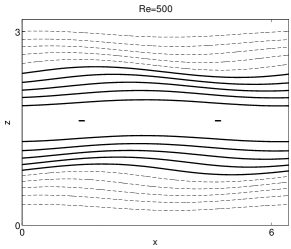
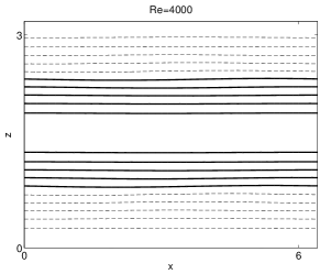
Figure 6: Contour plots of the streamwise velocity at $y=0$. The plots correspond to $D1$, $C1$, and $C4$. Contour lines are drawn at $12$ equispaced values between the maximum and minimum streamwise velocity in the slice. The lines are solid for positive values and dashed for negative values. The minimums are $-0.1922,-0.3969,-0.3833$ and the maximums are $0.4146,0.3969,0.3833$. In each plot the maximum occurs in the widest gap between the solid lines.

A notable feature of the solutions of Tables 1, 2 and 3 is that the solutions are streaky. This feature is illustrated in Figure 6. The contour lines for the streamwise velocity are approximately parallel to the $x$ axis, but the streamwise velocity varies in a pronounced way in the $z$ direction. We observe that $D1$ is less streaky than $C1$. The contour lines become much straighter when we go from $C1$ to $C4$. This increase in streakiness with $Re$ is in accord with the asymptotic theory sketched in [21].

To show that these solutions are not fully turbulent, we begin by describing the use of frictional or wall units [10]. The mean shear at the wall, which is denoted by $\bigl{<}\frac{\partial u}{\partial y}\bigl{|}_{y=1}\bigr{>}$, is the basis for frictional units. The frictional units for velocity and length are given by

$$u_{f}=\sqrt{\nu\Bigl{<}\frac{\partial u}{\partial y}\Bigl{|}_{y=1}\Bigr{>}}\quad\quad\text{and}\quad\quad l_{f}=\nu/u_{f},$$

respectively. If the width of the channel is $L$, the frictional Reynolds number is given by $Re_{\tau}=Lu_{f}/\nu=L/l_{f}$. The width of the channel in frictional units equals the frictional Reynolds number. The use of frictional units is signaled by using $+$ as a superscript.

The use of frictional units is necessary to state some remarkable properties of turbulent boundary layers. If $y^{+}$ measures the distance from the wall and $<\!\!u\!\!>^{+}$ is the mean streamwise velocity in frictional units, after making $<\!\!u\!\!>^{+}=0$ at $y^{+}=0$ by shifting the mean velocities if necessary, then $<\!\!u\!\!>^{+}\approx y^{+}$ in the viscous sublayer. The viscous sublayer is about $5$ frictional units thick. The buffer layer extends from $5$ to about $30$ units. It is followed by the logarithmic layer where $<\!\!u\!\!>^{+}\approx A\log y^{+}+B$, for constants $A$ and $B$. These relationships between $<\!\!u\!\!>^{+}$ and $y^{+}$ have been confirmed in numerous experiments and in some computations. The experiments are of a very diverse nature as discussed in [10], and it is remarkable that such a simple relationship holds across all those experiments.

There are other relationships that govern the dependence of quantities such as turbulence intensities or turbulent energy production on the distance from the wall. These relationships also characterize turbulent boundary layers. To show that the $C$ and $D$ solutions are not fully turbulent, we will use plots of turbulent energy production. Turbulent energy production equals

$$-<\!\!u^{\ast}v^{\ast}\!\!>\frac{\partial<\!\!u\!\!>}{\partial y},$$

where $u^{\ast}=u-<\!\!u\!\!>$ and $v^{\ast}=v-<\!\!v\!\!>$ are the fluctuating components of the streamwise and wall-normal velocities and $<\!\!u\!\!>$ is the mean streamwise velocity. Turbulent energy production is easy to measure experimentally and shows a very sharp peak in the buffer region of turbulent boundary layers [6]. This sharp peak has intrigued experimentalists for a long time. In experiments, the means are calculated by averaging pointwise measurements over long intervals of time. The means involved in the definition of turbulent energy production will be computed by averaging in the $x$ and $z$ directions.

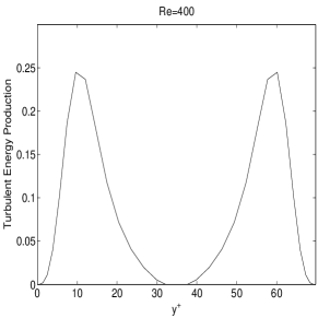
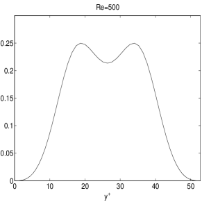
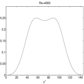
Figure 7: The plots show the dependence of turbulent energy production in frictional units on $y^{+}$ for a turbulent steady solution, $C1$, and $C4$.

Figure 7 shows plots of turbulent energy production against $y^{+}$, the distance from the upper wall in frictional units. In each plot, $y^{+}$ varies from $0$ to the channel width. The first plot is for a turbulent steady solution of plane Couette flow at $Re=400$. The data for the velocity field of that solution is from [20]. The second and third plots are for $C1$ and $C4$, respectively. The first plot is strikingly different from the other two. In the first plot, we notice that turbulent energy production peaks inside the buffer layer and then falls off sharply, in a way that is typical of turbulent boundary layers. The second and third plots correspond to higher $Re$, yet the peak occurs farther away from the wall in frictional units and there is no sharp fall-off. The plots for $D1$ and $D2$ are not shown. Those plots are similar to the ones for $C1$ and $C4$ in that they do not match what we expect for turbulent boundary layers. A notable difference is that the plots for $D1$ and $D2$ are not symmetric about the center of the channel. Thus the $C$ and $D$ solutions exhibit some aspects of near-wall turbulence such as the formation of streaks, but do not exhibit many other aspects.

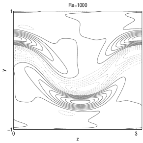
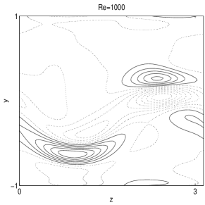
Figure 8: Contour plots of the streamwise vorticity at $x=\pi$. The contour lines are equispaced between $-0.11$ and $0.13$ for the first plot, which corresponds to $C2$, and between $-0.19$ and $0.17$ for the second plot, which corresponds to $D2$. The lines are dotted for negative values of streamwise vorticity.

Figure 8 is another illustration of the qualitative similarity between the $C$ and $D$ solutions. In both plots of Figure 8, one may observe a region near the center of the channel where the streamwise vorticity varies rapidly. Those regions correspond to the critical layer discussed in [21].

6 Conclusion

We verified the dynamical picture for transition to turbulence given in Figure 1 for certain disturbances. The third type of disturbance considered in Section 4.3 shows that that picture does not hold for all disturbances. A more exhaustive study of different types of disturbances of the laminar solution would be desirable.

We found (along with Wang et al.​​ [21]) that the $B$ or $C$ solutions become less unstable as $Re$ increases. This was an unexpected finding. Even a good heuristic explanation of this trend would be interesting.

Transition to turbulence computations would be good targets for reduced dimension methods. Reduced dimension methods are diverse in nature. Although this is not the place to review them, we believe the intricate dynamics of transition of turbulence featuring steady solutions, traveling waves, thresholds and various types of disturbances makes it non-trivial to reduce dimension. A valid way to reduce dimension must capture the dynamics correctly and not introduce spurious artifacts. It has been known since the work of Orszag and Kells [13] that under-resolved spatial discretizations lead to spurious transitions.

It is important to connect transition computations to experiments. However, connecting transition computations to experiments is impeded by two problems. Firstly, the experiments are performed in much larger domains to eliminate boundary effects. The numerical methods reviewed and discussed in Section 2 ought to be able to handle at least $10$ million degrees of freedom with a good parallel implementation. Therefore it seems that computations can be performed in much larger domains (i.e., domains with larger $\Lambda_{x}$ and $\Lambda_{z}$) and that this problem can be overcome. Secondly, it is very difficult to imagine a way to reproduce the sort of disturbances that have been considered in the computational literature in experiments. The disturbances used in experiments are of a different sort. For instance, one type of disturbance is to inject fluid from the walls. The best way to reconcile this disparity between computation and experiment might be to carry out computations using good models of laboratory disturbances.

7 Acknowledgments

The author thanks B. Eckhardt, J.F. Gibson, N. Lebovitz, L.N. Trefethen, and F. Waleffe for helpful discussions. This work was supported by the NSF grant DMS-0407110 and by a research fellowship from the Sloan Foundation.

References

- [1] D. Acheson. Elementary Fluid Dynamics. Oxford University Press, Oxford, 1990.
- [2] K.H. Bech, N. Tillmark, P.H. Alfredsson, and H.I. Andersson. An investigation of turbulent plane Couette flow at low Reynolds number. Journal of Fluid Mechanics, 286:291–325, 1995.
- [3] A. Cherhabili and U. Eherenstein. Finite-amplitude equilibrium states in plane Couette flow. Journal of Fluid Mechanics, 342:159–177, 1997.
- [4] J.F. Gibson, J. Halcrow, and P. Cvitanović. Visualizing the geometry of state space in plane Couette flow. Journal of Fluid Mechanics, 2007. Submitted. Available at www.arxiv.org.
- [5] G. Kawahara. Laminarization of minimal plane Couette flow: going beyond the basin of attraction of turbulence. Physics of Fluids, 17:art. 041702, 2005.
- [6] S.J. Kline, W.C. Reynolds, F.A. Schraub, and P.W. Rundstadler. The structure of turbulent boundary layers. Journal of Fluid Mechanics, 30:741–773, 1967.
- [7] G. Kreiss, A. Lundbladh, and D.S. Henningson. Bounds for threshold amplitudes in subcritical shear flows. Journal of Fluid Mechanics, 270:175–198, 1994.
- [8] M. Lagha, T.M. Schneider, F. De Lillo, and B. Eckhardt. Laminar-turbulent boundary in plane couette flow. 2007. preprint.
- [9] A. Lundbladh, D.S. Henningson, and S.C. Reddy. Threshold amplitudes for transition in channel flows. In M.Y. Hussaini, T.B. Gatski, and T.L. Jackson, editors, Turbulence and Combustion. Kluwer, Holland, 1994.
- [10] A.S. Monin and A.M. Yaglom. Statistical Fluid Mechanics. The MIT Press, Cambridge, 1971.
- [11] M. Nagata. Three dimensional finite amplitude solutions in plane Couette flow: bifurcation from infinity. Journal of Fluid Mechanics, 217:519–527, 1990.
- [12] M. Nagata. Three-dimensional traveling-wave solutions in plane Couette flow. Physical Review E, 55:2023–2025, 1997.
- [13] S.A. Orszag and L.C. Kells. Transition to turbulence in plane Poiseuille and plane Couette flow. Journal of Fluid Mechanics, 96:159–205, 1980.
- [14] T.M. Schmiegel and B. Eckhardt. Fractal stability border in plane couette flow. Physical Review letters, 79:5250, 1997.
- [15] T.M. Schneider, B. Eckhardt, and J.A. Yorke. Turbulence transition and edge of chaos in pipe flow. Physical Review Letters, 99:034502, 2007.
- [16] L.N. Trefethen, A.E. Trefethen, S.C. Reddy, and T.A. Driscoll. Hydrodynamic stability without eigenvalues. Science, 261:578–584, 1993.
- [17] D. Viswanath. Recurrent motions within plane Couette turbulence. Journal of Fluid Mechanics, 580:339–358, 2007.
- [18] F. Waleffe. Three-dimensional coherent states in plane shear flows. Physical Review Letters, 81:4140–4143, 1998.
- [19] F. Waleffe. Exact coherent structures in channel flow. Journal of Fluid Mechanics, 435:93–102, 2001.
- [20] F. Waleffe. Homotopy of exact coherent structures in plane shear flows. Physics of Fluids, 15:1517–1534, 2003.
- [21] J. Wang, J.F. Gibson, and F Waleffe. Lower branch coherent states in shear flows: transition and control. Physical Review Letters, 98:204501, 2007.