Evolutionary game dynamics in inhomogeneous populations

Abstract

To our knowledge, the populations are generally assumed to be homogeneous in the traditional approach to evolutionary game dynamics. Here, we focus on the inhomogeneous populations. A simple model which can describe the inhomogeneity of the populations and a microscopic process which is similar to Moran Process are presented. By studying the replicator dynamics, it is shown that this model also keeps the fixed points unchanged and can affect the speed of converging to the equilibrium state. The fixation probability and the fixation time of this model are computed and discussed. In the inhomogeneous populations, there are different situations that characterize the time scale of evolution; and in each situation, there exists an optimum solution for the time to the equilibrium points, respectively. Moreover, these results on the speed of evolution are valid for infinite and finite populations.

1 Introduction

Evolutionary game theory has been successfully founded and applied to the study of biology, economics, and social sciences by Maynard Smith [1]. Originally, evolutionary game theory was formulated in terms of infinite populations and the corresponding replicator dynamics. Consider two strategies A and B in a population engaged in a game with payoff matrix

$$\begin{array}[]{cccccccc}&&A&&B\\ A&&a&&~{}b.\\ B&&c&&d\\ \end{array}$$

A typical assumption is that individuals meet each other at random in infinitely large, well-mixed populations. The fitness (or payoff) of A and B players are respectively given by

$$\begin{array}[]{cccccc}f_{A}=ax+b(1-x),\\ f_{B}=cx+d(1-x),\end{array}$$ (2)

where $x$ is the frequency of A players and $1-x$ is the frequency of B players. The average fitness of the population is

$$\bar{f}=xf_{A}+(1-x)f_{B}.$$ (3)

The standard replicator equation which describes evolutionary dynamics in a infinite population takes the form [2, 3]

$$\dot{x} = x(f_{A}-\bar{f})$$ (4)

$$= x(1-x)[(a-b-c+d)x-(d-b)].$$

The equilibrium points are either on the boundary or in the interior. There are four generic outcomes [4, 5, 6]:
(1) If $a>c$ and $b>d$ then A dominates B; the only stable equilibrium is $x=1$.
(2) If $a<c$ and $b<d$ then B dominates A; the only stable equilibrium is $x=0$.
(3) If $a>c$ and $b<d$ then A and B are bi-stable; both $x=0$ and $x=1$ are stable equilibria; there is an unstable equilibrium at $x=(d-b)/(a-b-c+d)$.
(4) If $a<c$ and $b>d$ then A and B co-exist; both $x=0$ and $x=1$ are unstable equilibria; the only stable equilibrium is given by $x=(d-b)/(a-b-c+d)$.

The standard replicator dynamics hold in the limit of infinite population size. In fact, any real population has finite size and also computer simulations in structured or unstructured populations always deal with finite populations [7, 8, 9, 10]. Therefore, it is natural to study evolutionary game dynamics in finite populations. In most approaches for finite population size, each individual interacts with each other individual in the well-mixed, homogeneous populations. Moreover, stochastic processes have been introduced to study evolutionary dynamics in finite populations. Recently, in unstructured finite populations different mechanisms are applied to study game dynamics, such as Moran Process, Pairwise Comparison Process, Wright-Fisher Process, local information, mutation, discounting and active linking [11, 12, 13, 14, 15, 16, 17].

To our best knowledge, in the aforementioned approaches to evolutionary game theory, they are all based on the simplifying assumptions that the populations are homogeneous and each individual, which is engaged in symmetric game, is identical to strategy update. In fact, biological agents in many real populations are non-identical to their abilities to competition, survival and reproduction. For instance, the difference in sex, male or female, plays a significant role in group dominance. The age, old or young; the strength, strong or weak, etc, are also factors affecting the individuals’ competition and cooperation. Thus, we here relax the simplifying assumptions and consider that the populations are inhomogeneous. In our scenario, we aim to investigate the inhomogeneity’s effect in evolutionary game dynamics. The remainder of this paper is organized as follows: A simple model is constructed to describe the inhomogeneity of the populations and a stochastic process for evolutionary game theory is introduced in section 2. And then analytical results and corresponding simulations of the model are provided in section 3. Finally, conclusions are made in section 4.

2 The Model

In this model, the populations are well-mixed and each player interacts with each other player. To describe the inhomogeneity of the populations, we just assume that two types of players are distributed randomly in the populations (just like male and female individuals in a population) [18, 19]. For simplicity, we use E to denote one type players and F to denote the other type players. Every player has only one type and their distribution is fixed later on. The concentration of players E and F are denoted by $v(0\leq v\leq 1)$ and $1-v$. All individuals just follow A or B strategies no matter what types they are. And when players E interact with other players, the payoff of players E will be strengthened no matter what strategies players E follow; while the payoff of players F will keep unchanged no matter what strategies players F follow when players F interact with other players. Now, suppose the population consists of $N$ players. The number of players using strategy A is given by $i$, the number of players using strategy B is given by $N-i$. If every player interacts with every other player, the average payoff of A and B are respectively given from a mean-field theory

$$\begin{array}[]{ccccc}\Pi^{A}_{i}=\frac{a(i-1)+b(N-i)}{N-1}[vq_{1}+(1-v)],\\ \Pi^{B}_{i}=\frac{ci+d(N-i-1)}{N-1}[vq_{1}+(1-v)],\end{array}$$ (5)

where the parameter $q_{1}(q_{1}>1)$ characterizes the rates of increased payoff of players E. Therefore, the average payoff of the population at the state is given

$$<\Pi>=[i\Pi^{A}_{i}+(N-i)\Pi^{B}_{i}]/N.$$ (6)

Then, the average fitness of strategies A and B are respectively given by [20]

$$\begin{array}[]{cccccc}f_{A}=1-w+w\Pi^{A}_{i},\\ f_{B}=1-w+w\Pi^{B}_{i},\end{array}$$ (7)

where $w$ measures the intensity of selection. Strong selection means $w=1$; weak selection means $w\ll 1$.

We now describe the selection mechanism process as follows: In each time step, an individual is chosen with a probability proportional to its fitness; a second individual is selected randomly. Then the second individual switches to the first one’s strategy. Moreover, if the second individual is a player E, it will weaken the probability to switch to the first one’s strategy; otherwise, it will keep the probability to switch to the first one’s strategy. And we write the probability that the number of A individuals increases from $i$ to $i+1$ as

$$T^{+}(i) = \frac{if_{A}}{if_{A}+(N-i)f_{B}}\cdot\frac{N-i}{N}\cdot[vq_{2}+(1-v)]$$ (8)

$$= \frac{1-w+w\Pi^{A}}{1-w+w<\Pi>}\cdot\frac{i}{N}\cdot\frac{N-i}{N}\cdot[vq_{2}+(1-v)],$$

where the parameter $q_{2}$ characterizes the strength of reduced switching activity if the second individual is occupied by an individual of type E. Since players E can strengthen their payoff, they are not sensitive to switch their strategies, therefore, we set $q_{2}<1$ . The probability that the number of A individuals decreases from $i$ to $i-1$ is

$$T^{-}(i)=\frac{1-w+w\Pi^{B}}{1-w+w<\Pi>}\cdot\frac{i}{N}\cdot\frac{N-i}{N}\cdot[vq_{2}+(1-v)].$$ (9)

Consequently, the probability that the number of A individuals remains constant is $T(i)=1-T^{+}(i)-T^{-}(i)$. Since $T^{-}(N)=0$ and $T^{+}(0)=0$, this process has absorbing states at $i=0$ and $i=N$. For large populations, a Langevin equation can approximately describe this process [11]

$$\begin{array}[]{cccccc}\dot{x}=a(x)+b(x)\varepsilon,\\ a(x)=T^{+}(x)-T^{-}(x),\\ b(x)=\sqrt{[T^{+}(x)+T^{-}(x)]/N},\end{array}$$

where $x=\frac{i}{N}$ is the fraction of A, $a(x)$ is the drift term, $b(x)$ is the diffusion term and $\varepsilon$ is uncorrelated Gaussian noise. For large $N$, $b(x)$ vanishes with $1/\sqrt{N}$, this equation becomes

$$\dot{x} = x(1-x)\cdot\frac{w[\Pi^{A}(x)-\Pi^{B}(x)]}{1-w+w<\Pi(x)>}\cdot[vq_{2}+(1-v)]$$ (11)

$$\triangleq F(v)\cdot x(x-1)[(b+c-a-d)x+(d-b)]/G(w,x,v),$$

where

$$F(v) = [vq_{1}+(1-v][vq_{2}+(1-v)]$$

$$= (q_{1}-1)(q_{2}-1)v^{2}+(q_{1}+q_{2}-2)v+1,$$

$$G(v,x,w) = \frac{1-w}{w}+[vq_{1}+(1-v)]\cdot$$

$$[(a-b-c+d)x^{2}+(b+c-2d)x+d].$$

(11) is the replicator dynamics equation for this model. For $v=0$, the replicator dynamics equation for the Moran Process in homogeneous populations is recovered. For $0<v<1$, inhomogeneity is introduced in the system as there are two types of players in populations. Subsequently, the replicator dynamics, the fixation probability and the fixation time of this model are to be investigated and discussed for different values of the parameters.

3 Analytical Results and Corresponding Simulations

For the Moran Process in homogeneous populations,

$$\dot{x}=x(x-1)[(b+c-a-d)x+(d-b)]/\Gamma(x,w),$$ (12)

where $\Gamma(x,w)=\frac{1-w}{w}+[(a-b-c+d)x^{2}+(b+c-2d)x+d]$. Comparing with (4) and (12), (11) also has the three same equilibria: $x=0$, $1$ and $(d-b)/(a-b-c+d)$ and keeps the fixed points unchanged. Moreover, there are apparently four same generic cases for the stable equilibrium points to (4) by studying (11). To illustrate this, let us consider an example. Consider the payoff matrix

$$\begin{array}[]{cccccccc}&&A&&B\\ A&&0.3&&0.5~{}.\\ B&&0.1&&0.2\\ \end{array}$$

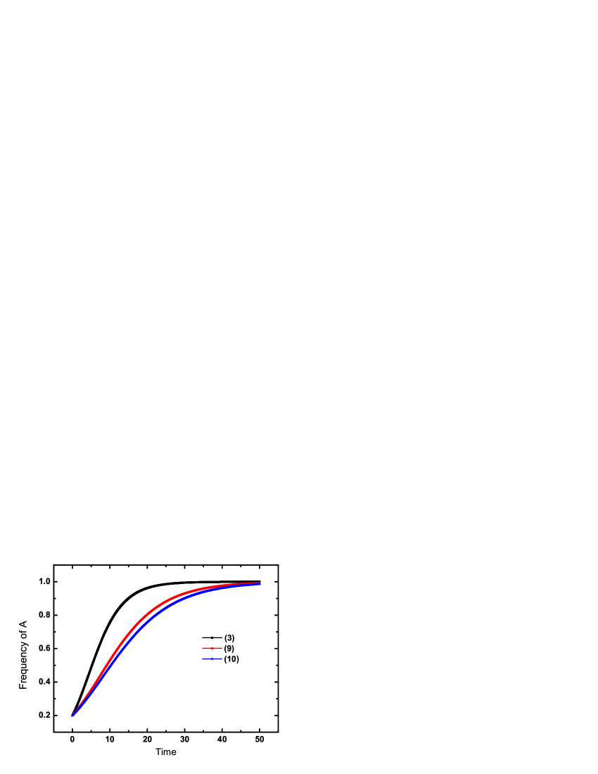
Figure 1: Frequency of A as a function of time for different equations from an initial state with $20\%$ A, given fixed values of $q_{1}=2$, $q_{2}=0.4$ and $w=0.4$ for (11) and (12).

The fitness of A is greater than the fitness of B in this example. Hence, we say that A dominates B. Figure 1 shows the evolution from a state with $20\%$ A into the end state with all A. Since $a=0.3>c=0.1$ and $b=0.5>d=0.2$, figure 1 confirms the theoretical predictions.

In fact, the differences among the three dynamics equations amount to a dynamics rescaling of time. And $F(v)$ and $G(v,x,w)$ in (11) are factors influencing the time scale only. They would affect only the speed of evolution, but would not influence the long-run behavior. Then, we would like to show that how they affect the time scale for different values of the parameters. In this model for the fixed values of $q_{1}$, $q_{2}$ and $w$, $G(v,x,w)\approx\frac{1-w}{w}$ is constant with weak selection, then only $F(v)$ can influence the time scale for the variable $v$. Here, $F(v)$ has a maximum at $v=v_{c}$ for different $v\in[0~{}1]$, and $F(v)=(q_{1}-1)(q_{2}-1)v^{2}+(q_{1}+q_{2}-2)v+1\leq F(v_{c})$, then there exists the optimum $v_{c}$ to converge fastest to the equilibrium state. Since $(q_{1}-1)(q_{2}-1)<0~{}(q_{1}>1,q_{2}<1)$, there are three cases for different relationships between $q_{1}$ and $q_{2}$:

$$F(v) = (q_{1}-1)(q_{2}-1)[v+\frac{q_{1}+q_{2}-2}{2(q_{1}-1)(q_{2}-1)}]^{2}+$$

$$1-\frac{(q_{1}+q_{2}-2)^{2}}{4(q_{1}-1)(q_{2}-1)}.$$

(1) If $q_{1}+q_{2}<2$, then $F(v)$ has its maximum at $v_{c}=0$.
(2) If $2\leq q_{1}+q_{2}<2q_{1}q_{2}$, then $F(v$ has its maximum at $v_{c}=1$.
(3) If $q_{1}+q_{2}\geq 2q_{1}q_{2}$, then $F(v)$ has its maximum at $v_{c}=\frac{2-q_{1}-q_{2}}{2(q_{1}-1)(q_{2}-1)}$.
Especially, the interesting relationship between $q_{1}$ and $q_{2}$ for $q_{1}>1$ and $q_{2}<1$ is $q_{1}q_{2}=1$. In this case, then $q_{1}+q_{2}>2q_{1}q_{2}=2$ and there is only one outcome for $v_{c}$: $v_{c}=\frac{2-q_{1}-q_{2}}{2(q_{1}-1)(q_{2}-1)}=0.5$.

The four outcome predictions, which can respectively reflect the four relationships between $q_{1}$ and $q_{2}$, are found from the replicator dynamics equation, thus they are justified for infinite or large finite populations. In other words, it can converge fastest to the equilibrium state when $v=v_{c}$ for infinite populations. However, in finite populations, if the mean time to fixation becomes very large, the model may be limited interest, therefore, discussion on the fixation time $T_{v}$ is an interesting topic. Here, whether the fixation time $T_{v}$ in finite populations has a minimum at $v_{c}$ respectively corresponding to the four situations in infinite populations is a more interesting topic. Indeed, the four outcome predictions for infinite populations are still valid for small finite populations. For finite populations, $T_{v}$ means that the time from an initial state $x_{0}$ to the equilibrium state and can be calculated by [13, 21]

$$T_{v}=N\int_{0}^{1}t(x,x_{0})dx,$$ (14)

where

$$t(x,x_{0})=\frac{2[S(1)-S(x_{0})]S^{2}(x)}{b^{2}(x)S(1)S(x_{0})}\cdot\exp{[\int_{0}^{x}\frac{2a(y)}{b^{2}(y)}dy]},(0\leq x\leq x_{0})$$

$$t(x,x_{0})=\frac{2[S(1)-S(x)]S(x)}{b^{2}(x)S(1)}\cdot\exp{[\int_{0}^{x}\frac{2a(y)}{b^{2}(y)}dy]},(x_{0}\leq x\leq 1)$$

and

$$S(x)=\int_{0}^{x}\exp{[-\int_{0}^{y}\frac{2a(z)}{b^{2}(z)}dz]}dy.$$

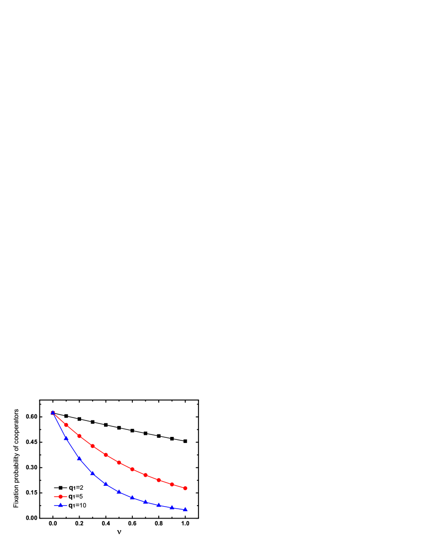
Figure 2: Fixation probability of $k=80$ cooperators in a Prisoner’s Dilemma as a function of $v$ for different rates $q_{1}$, given a fixed value of $N=100$.

Figure 3: The fixation time $T_{v}$ as a function of $v$ for $N=1000$, given different relationships between $q_{1}$ and $q_{2}$: (a). $q_{1}=1.2$ and $q_{2}=0.6$; in this case, $v_{c}=0$. (b). $q_{1}=2$ and $q_{2}=0.8$; in this case, $v_{c}=1$. (c). $q_{1}=8.5$ and $q_{2}=0.25$; in this case, $v_{c}=0.6$. (d). $q_{1}=5$ and $q_{2}=0.2$; in this case, $v_{c}=0.5$

As this can be done numerically in general, the corresponding simulation results are shown below. Before computing the fixation time, let us first investigate the fixation probability for this model. The fixation probability $\phi_{k}$ with $k$ players using strategy A is given by [22]

$$\phi_{k} = \frac{1+\sum_{j=1}^{k-1}\prod_{i=1}^{j}\frac{T^{-}(i)}{T^{+}(i)}}{1+\sum_{j=1}^{N-1}\prod_{i=1}^{j}\frac{T^{-}(i)}{T^{+}(i)}}$$

$$= \frac{\displaystyle 1+\sum_{j=1}^{k-1}\prod_{i=1}^{j}\frac{(1-w)(N-1)+w(vq_{1}+1-v)[ci+d(N-i-1)]}{(1-w)(N-1)+w(vq_{1}+1-v)[a(i-1)+b(N-i)]}}{\displaystyle 1+\sum_{j=1}^{N-1}\prod_{i=1}^{j}\frac{(1-w)(N-1)+w(vq_{1}+1-v)[ci+d(N-i-1)]}{(1-w)(N-1)+w(vq_{1}+1-v)[a(i-1)+b(N-i)]}}.$$

Now let us take the Prisoner’s Dilemma for example. In most papers, the Prisoner’s Dilemma is determined by the payoff matrix

$$\begin{array}[]{cccccccc}&&&C&&D\\ C&&&b-c&&-c.\\ D&&&b&&0\\ \end{array}$$

To assure that the fitness of C and D are always positive, the payoff matrix becomes

$$\begin{array}[]{cccccccc}&&&C&&D\\ C&&&b-c&&-c\\ D&&&b&&0\\ \end{array}~{}~{}~{}\Rightarrow~{}~{}~{}\begin{array}[]{cccccccc}&&&C&&D\\ C&&&b&&0.\\ D&&&b+c&&c\\ \end{array}$$

In the following simulation results, the initial frequency of cooperators is $80\%$, and we set $b=3$, $c=2$ and $w=0.0001$. In figure 2, we show the fixation probability of a Prisoner’s Dilemma starting with $80\%$ cooperators. Clearly, cooperators are always dominated by defectors. It shows that stronger rates $q_{1}$ decrease the fixation probability of cooperators and the fixation probability of cooperators monotonically decreases when the value of the parameter $v$ increases with a given fixed $q_{1}$. These results can be understood in the following way. When the values of $q_{1}$ or $v$ increase, it results in that the temperature of selection is enhanced. For the Prisoner’s Dilemma, the average payoff of cooperators is less than the average payoff of defectors. Therefore, the fixation probability of cooperators decreases for the Prisoner’s Dilemma when the temperature of selection is increased [19]. Moreover, we have found that the fixation probability has nothing to do with the strength of switching activity $q_{2}$ from (3). In figure 3, we show the fixation time of a Prisoner’s Dilemma starting with $80\%$ cooperators for $N=1000$. The fixation time from (14) for different situations are computed, respectively. In figure 3(a), $q_{1}+q_{2}=1.8<2$. In this case, $T_{v}$ has its minimum at $v=0$. And we observe that $v_{c}=0$ from figure 3(a). In figure 3(b), $2<q_{1}+q_{2}=2.8<3.2=2q_{1}q_{2}$. In this case, $T_{v}$ has its minimum at $v=1$. And we observe that $v_{c}=1$ from figure 3(b). In figure 3(c), $2q_{1}q_{2}=4.25<q_{1}+q_{2}=8.75$, In this case, $T_{v}$ has its minimum at $v=\frac{2-8.5-0.25}{2\times(8.5-10\times(0.25-1)}=0.6$. And we observe that $v_{c}=0.6$ from figure 3(c). In figure 3(d), $2<q_{1}+q_{2}=5.2$ and $q_{1}q_{2}=1$. In this case, $T_{v}$ has its minimum at $v=0.5$. And we observe that $v_{c}=0.5$ from figure 3(d). These results for finite populations are totally in very good agreement with theoretical predictions for infinite populations and these figures confirm that the fixation time $T_{v}$ also has its minimum at $v_{c}$. Moreover, these results for the fixation time in finite populations are still valid even if $w$ does not satisfy the condition: $w\ll 1$.

4 Conclusions

To sum up, we have studied the evolutionary game dynamics in inhomogeneous populations. We have provided a model by description of a microscopic process which is similar to Moran Process. Comparing with standard replicator and Moran Process dynamics, it also keeps the fixed points unchanged. Nevertheless, this can affect the speed of converging to the equilibrium state. We have also calculated the fixation probability and the fixation time, and found that there exists an optimum solution to converge fastest to the stable equilibria. This result requires no limiting assumption on population size. As is known, how to decrease the mean time to the fixed state from an initial state is an important quantity [23]. From this perspective, our results on inhomogeneous populations may shed light on this issue.

References

References

- [1] J. M. Smith 1982 Evolution and the Theory of Games (London: Cambridge University Press)
- [2] P. D. Taylor and L. Jonker 1978 Math. Biosci. 40 145
- [3] J. Hofbauer and K. Sigmund 1998 Evolutionary Games and Population Dynamics (London: Cambridge University Press)
- [4] C. Taylor, D. Fudenberg, A. Sasaki and M. A. Nowak 2004 Bull. Math. Biol. 66 1621
- [5] L. A. Imhof and M. A. Nowak 2006 J. Math. Biol. 52 667
- [6] C. Taylor and M. A. Nowak 2006 Theor. Popul. Biol. 69 243
- [7] C. Hauert and M. Doebeli 2004 Nature 428 643
- [8] H. Ohtsuki, C. Hauert, E. Lieberman and M. A. Nowak 2006 Nature 441 502
- [9] F. C. Santos and J. M. Pacheco 2005 Phys. Rev. Lett.95 098104
- [10] J. Vukov, G. Szabó and A. Szolnoki 2006 Phys. Rev. E 73 067103
- [11] A. Traulsen, J. C. Claussen and C. Hauert 2005 Phys. Rev. Lett.95 238701
- [12] A. Traulsen, M. A. Nowak and J. M. Pacheco 2006Phys. Rev. E 74 011909
- [13] A. Traulsen, J. M. Pacheco and L. A. Imhof 2006 Phys. Rev. E 74 021905
- [14] C. Hauert, F. Michor, M. A. Nowak and M. Doebeli 2006 J. Theor. Biol. 239 195
- [15] D. Fudenberg, M. A. Nowak, C. Hauert and L. A. Imhof 2006 Theor. Popul. Biol. 70 262
- [16] M. Willensdorfer and M. A. Nowak 2005 J. Theor. Biol. 237 355
- [17] C. P. Roca, J. A. Cuseta and A. Sánchez 2006 Phys. Rev. Lett.97 158801
- [18] A. Szolnoki and G. Szabó 2006 Preprint q-bio.PE/0610001
- [19] A. Traulsen, M. A. Nowak and J. M. Pacheco 2007 J. Theor. Biol. 244 349
- [20] M. A. Nowak, A. Sasaki, C. Taylor and D. Fudenberg 2004 Nature 428 646
- [21] W. J. Ewens 1979 Mathematical Population Genetics (Berlin: Springer)
- [22] S. Karlin and H. M. A. Taylor 1975 A first course in stochastic process (New York: Academic press)
- [23] C. Taylor, Y. Iwasa and M. A. Nowak 2006 J. Theor. Biol. 243 245