Weakly nonlinear waves in magnetized plasma with a slightly non-Maxwellian electron distribution. Part 2. Stability of cnoidal waves

Abstract

We determine the growth rate of linear instabilities resulting from long-wavelength transverse perturbations applied to periodic nonlinear wave solutions to the Schamel-Korteweg-de Vries-Zakharov-Kuznetsov (SKdVZK) equation which governs weakly nonlinear waves in a strongly magnetized cold-ion plasma whose electron distribution is given by two Maxwellians at slightly different temperatures. To obtain the growth rate it is necessary to evaluate non-trivial integrals whose number is kept to minimum by using recursion relations. It is shown that a key instance of one such relation cannot be used for classes of solution whose minimum value is zero, and an additional integral must be evaluated explicitly instead. The SKdVZK equation contains two nonlinear terms whose ratio $b$ increases as the electron distribution becomes increasingly flat-topped. As $b$ and hence the deviation from electron isothermality increases, it is found that for cnoidal wave solutions that travel faster than long-wavelength linear waves, there is a more pronounced variation of the growth rate with the angle $\theta$ at which the perturbation is applied. Solutions whose minimum value is zero and travel slower than long-wavelength linear waves are found, at first order, to be stable to perpendicular perturbations and have a relatively narrow range of $\theta$ for which the first-order growth rate is not zero.

1 Introduction

In Part 1 (Allen et al. 2007) we considered solitary wave solutions of a modified version of the Zakharov-Kuznetsov (ZK) equation which, in a frame moving at speed $V$ above the speed of long-wavelength linear waves, takes the form

$$u_{t}+(u+bu^{1/2}-V)u_{x}+\nabla^{2}u_{x}=0$$ (1.1)

where the subscripts denote derivatives. We referred to this equation as the Schamel-Korteweg-de Vries-Zakharov-Kuznetsov (SKdVZK) equation as it contains both the quadratic nonlinearity of the KdV equation and the half-order nonlinearity of the Schamel equation. The equation governs weakly nonlinear ion-acoustic waves in a plasma permeated by a strong uniform magnetic field in the $x$-direction. The plasma contains cold ions and two populations of hot electrons, one free and the other trapped by the wave potential, whose effective temperatures differ slightly. In (1.1) $u$ is proportional to the electrostatic potential, and $b=(1-T_{\rm ef}/T_{\rm et})/\sqrt{\pi}$ where $T_{\rm ef}$ and $T_{\rm et}$ are the effective temperatures of the free and trapped electrons, respectively. As $b$ increases, the electron distribution becomes less peaked. A flat-topped distribution is in accordance with numerical simulations and experimental observations of collisionless plasmas (Schamel 1973). For further background to the physical basis and applicability of the SKdVZK and related equations, reference should be made to Part 1.

The existence of planar solitary wave solutions to the SKdVZK equation and their stability to transverse perturbations was addressed in Part 1. In this paper we turn to the study of planar cnoidal wave solutions to the equation. In Sec. 2 we show that a number of families of cnoidal wave solutions to the one-dimensional form of (1.1) exist, but not all can be expressed in closed form. Linear stability analysis of periodic solutions of the SKdVZK equation with respect to transverse perturbations is carried out in Sec. 3. Such an analysis has been carried out on cnoidal wave solutions of the ZK and SZK equations which contain single quadratic and half-order nonlinearities, respectively (Infeld 1985; Munro and Parkes 1999). However, as far as we are aware, such a calculation has not been performed before on an equation containing two nonlinear terms. The stability analysis leads to a nonlinear dispersion relation in the form of a cubic equation whose coefficients are finite-part integrals involving the unperturbed solution and its derivative. As the solutions contain elliptic functions the integrals are non-trivial. Recursion relations between the integrals are derived in order that only the simplest finite integrals need to be evaluated directly. For some types of solution it is shown that one instance of a recursion relation cannot be used and an extra integral must be found directly. In Sec. 4 we examine how the first-order coefficient of the growth rate found from the nonlinear dispersion relation depends on the type of cnoidal wave, the angle at which the perturbation is applied, and $b$. Our conclusions are presented in the final section.

2 Cnoidal wave solutions

To look for planar cnoidal wave solutions of permanent form travelling at speed $V$ above the long-wavelength linear wave speed we drop the $t$, $y$ and $z$ dependence in (1.1). Integrating once then gives

$$u_{xx}=\frac{C}{2}+Vu-\frac{2}{3}bu^{3/2}-\frac{1}{2}u^{2},$$ (2.2)

and multiplying by $2u_{x}$ and integrating once more yields

$$u_{x}^{2}=C_{0}+Cu+Vu^{2}-\frac{8}{15}bu^{5/2}-\frac{1}{3}u^{3}$$ (2.3)

where $C_{0}$ and $C$ are integration constants. Although from phase plane analysis it is clear that a number of families of periodic nonlinear waves exist, only when $C_{0}=0$ can closed-form solutions be obtained in general. Sketches of (2.3) for the various cases leading to periodic solutions when $C_{0}=0$ are shown in Fig. 1.

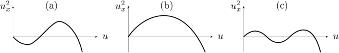
Figure 1: $(u,u_{x}^{2})$-sketches of (2.3) with $C_{0}=0$ showing existence of families of periodic wave solutions: (a) $C<0$, $V>0$ or $b<0$ (or both); (b) $C>0$; (c) $C>0$ for some $V<0$ and $b<0$.

After introducing the variable $r=\sqrt{u}$, (2.3) with $C_{0}\equiv 0$ reduces to

$$4r_{x}^{2}=g(r)\equiv h(r)+C,\qquad h(r)\equiv Vr^{2}-\frac{8b}{15}r^{3}-\frac{1}{3}r^{4}.$$ (2.4)

Possible forms of $g(r)$ for various $V$, $b$ and $C$ are sketched in Fig. 2. The $u^{1/2}$ term that appears in (1.1) must be interpreted as the positive square root and as a result we must restrict solutions of (2.4) to $r\geqslant 0$. In view of this, at first sight it would appear that nonlinear wave solutions to (2.4) that cross the line $r=0$ with positive $r_{x}^{2}$ would have to be discarded. However, since $u_{x}^{2}=r^{2}g(r)$, the $r\geqslant 0$ part of such a solution forms a complete closed loop that touches the origin in the ($u$$\geqslant$$0,u_{x})$-plane, as can be seen to occur in Fig. 1(b) and (c), and hence corresponds to a nonlinear wave solution with a minimum value of zero. Although for such solutions in the $(r,r_{x})$-plane $r_{x}$ jumps from a negative to an equal and opposite positive value at $r=0$, it is easily shown that $u$ and its derivatives are continuous there. The jump in the solution in the $(r,r_{x})$-plane means that the solutions are most simply expressed as functions extended by periodicity. Such solutions have already categorized for the Schamel equation (which contains the single half-order nonlinearity) in O’Keir and Parkes (1997). Schamel (1972) described them for the current equation but in the following they are presented in a more unified form.

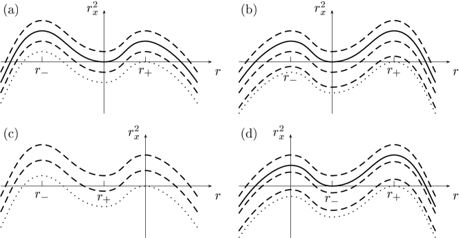
Figure 2: $(r,r_{x}^{2})$-sketches of (2.4) for (a) $V>0$, $b>0$ (b) $V>0$, $b<0$ (c) $-6b^{2}/25<V<0$, $b>0$ (d) $-6b^{2}/25<V<0$, $b<0$. Solid, dashed and dotted curves give rise to solitary wave, periodic nonlinear wave, and constant (linear limit) solutions, respectively.

The quartic $g(r)$ will always have a stationary point at $r=0$ and also at

$$r_{\pm}=\pm\sqrt{\left(\frac{3b}{5}\right)^{2}+\frac{3V}{2}}-\frac{3b}{5}$$ (2.5)

provided that $V>-6b^{2}/25$. From the sketches of $g(r)$ in Fig. 2, it is apparent that if $r_{+}$ is real and positive, nonlinear wave solutions will only occur if $C>-h(r_{+})$ and the linear wave limit corresponds to $C=-h(r_{+})$.

If $g(r)$ has four real roots, $r_{1}<r_{2}<r_{3}<r_{4}$, then solving (2.4) yields the cnoidal wave solution

$$u(x)=[r(x)]^{2}=\left(\frac{r_{4}+r_{1}\rho\mathop{\mathrm{sn}}\nolimits^{2}(\eta(x-x_{0})|m)}{1+\rho\mathop{\mathrm{sn}}\nolimits^{2}(\eta(x-x_{0})|m)}\right)^{2}$$ (2.6)

where

$$\rho\equiv\frac{r_{4}-r_{3}}{r_{3}-r_{1}},\qquad m\equiv\frac{r_{2}-r_{1}}{r_{4}-r_{2}}\,\rho,\qquad\eta\equiv\sqrt{\frac{(r_{4}-r_{2})(r_{3}-r_{1})}{48}},$$

and $x_{0}$ is an arbitrary phase. We will refer to this class of solution as being of type I. Note that when $V>0$, in the soliton limit $c=0$ we have $r_{3}=r_{2}=0$ and (2.6) then reduces to the conventional solitary wave solution given in Part 1.

When $b<0$, it can be seen from Fig. 2(b) and (d) that there are periodic wave solutions corresponding to a $g(r)$ with just two real roots for $-h(r_{+})<C<-h(r_{-})$ when $V>0$, and for $-h(r_{+})<C<0$ when $-6b^{2}/25<V<0$. If the two real roots are $r_{\rm u}$ and $r_{\rm l}$, with $r_{\rm u}>r_{\rm l}$, and the remaining two complex conjugate roots are $\alpha\pm{\rm i}\beta$, then solving (2.4) in this case gives what we call the type II solution,

$$u(x)=[r(x)]^{2}=\left(\frac{\displaystyle{(Ar_{\rm l}+Br_{\rm u})-(Ar_{\rm l}-Br_{\rm u})\mathop{\mathrm{cn}}\nolimits(\bar{\eta}(x-x_{0})|\bar{m})}}{\displaystyle{(A+B)-(A-B)\mathop{\mathrm{cn}}\nolimits(\bar{\eta}(x-x_{0})|\bar{m})}}\right)^{2},$$ (2.7)

where

$$A=\sqrt{(r_{\rm u}-\alpha)^{2}+\beta^{2}},\qquad B=\sqrt{(r_{\rm l}-\alpha)^{2}+\beta^{2}},$$

and

$$\bar{m}=\frac{(r_{\rm u}-r_{\rm l})^{2}-(A-B)^{2}}{4AB},\qquad\bar{\eta}=\sqrt{\frac{AB}{12}}.$$

We now turn our attention to the solutions written as periodically extended functions. For $V>0$ these occur when $c>0$. As in these cases there are only two real roots, these solutions take a similar form to (2.7). However, due to the jump in the $(r,r_{x})$-plane they must be written in the form

$$u(x)=\left(\frac{\displaystyle{(Ar_{\rm l}+Br_{\rm u})-(Ar_{\rm l}-Br_{\rm u})\mathop{\mathrm{cn}}\nolimits(\bar{\eta}\check{x}(\bar{\chi}/\bar{\eta})|\bar{m})}}{\displaystyle{(A+B)-(A-B)\mathop{\mathrm{cn}}\nolimits(\bar{\eta}\check{x}(\bar{\chi}/\bar{\eta})|\bar{m})}}\right)^{2},\quad\bar{\chi}=\mathop{\mathrm{cn}}\nolimits^{-1}\left(\frac{Ar_{\rm l}+Br_{\rm u}}{Ar_{\rm l}-Br_{\rm u}}\right)$$ (2.8)

where

$$\check{x}(p)\equiv(x-x_{0}+p\bmod 2p)-p.$$

These solutions have a period of $2\bar{\chi}/\bar{\eta}$ and for a given value of $V$ and $b$ have a larger amplitude than the solitary wave. We call these type II_pe solutions. When $b=0$ they reduce to an ordinary KdV equation cnoidal wave solution with a minimum value of zero.

From Fig. 2(c) and (d) it is clear that when $V<0$, smaller amplitude solutions that touch $u=0$ are also possible. When there are two real roots, (2.8) still applies, while if $b>0$ and there are four real roots, what we will refer to as the type I_pe solution results. It is similar to (2.6) but must be written as

$$u(x)=\left(\frac{r_{4}+r_{1}\rho\mathop{\mathrm{sn}}\nolimits^{2}(\eta\check{x}(\chi/\eta)|m)}{1+\rho\mathop{\mathrm{sn}}\nolimits^{2}(\eta\check{x}(\chi/\eta)|m)}\right)^{2},\quad\chi=\mathop{\mathrm{sn}}\nolimits^{-1}\sqrt{\frac{r_{4}}{r_{1}\rho}}.$$ (2.9)

When there are four real roots and $b<0$, the solution which has a minimum value of zero is the same as the above after making the interchanges $r_{4}\leftrightarrow r_{2}$ and $r_{3}\leftrightarrow r_{1}$.

3 Linear stability analysis

By using the small-$k$ expansion method (Rowlands 1969; Infeld 1985; Infeld and Rowlands 2000), we now investigate the linear stability of periodic waves to long-wavelength perturbations with wavevector $k(\cos\theta,\sin\theta\cos\varphi,\sin\theta\sin\varphi)$ where $\theta$ is the angle between the direction of the wavevector and the $x$-axis, and $\varphi$ is the azimuthal angle. We start from the ansatz

$$u=u_{0}(x)+\varepsilon\Phi(x){\rm e}^{{\rm i}k(x\cos\theta+y\sin\theta\cos\varphi+z\sin\theta\sin\varphi)-{\rm i}\omega t}$$ (3.10)

where $u_{0}(x)$ is a periodic solution to (1.1), $\varepsilon\!<\!\!<\!1$, and the eigenfunction $\Phi(x)$ must have the same period as $u_{0}(x)$. Substituting (3.10) into (1.1) and linearizing with respect to $\varepsilon$ gives

$$\frac{{\rm d}}{{\rm d}x}L\Phi={\rm i}\omega\Phi-{\rm i}k\cos\theta\,Q\Phi-3{\rm i}k\cos\theta\,\Phi_{xx}+k^{2}(1+2\cos^{2}\theta)\Phi_{x}+{\rm i}k^{3}\cos\theta\,\Phi$$ (3.11)

where

$$L\equiv\frac{{\rm d}^{2}}{{\rm d}x^{2}}+Q,\qquad Q\equiv u_{0}+bu^{1/2}_{0}-V,$$

and $\Phi$ and $\omega$ are written as the expansions,

$$\Phi = \Phi_{0}+k\Phi_{1}+\ldots,$$ (3.12)

$$\omega = \omega_{1}k+\omega_{2}k^{2}+\ldots\;.$$ (3.13)

For the remainder of the calculation we follow a similar procedure to that first given in Parkes (1993). After substituting (3.12) and (3.13) into (3.11) and equating coefficients of $k^{n}$ we obtain the sequence of equations

$$(L\Phi_{n})_{x}=R_{nx}(x)$$ (3.14)

in which the expressions for $R_{nx}$ are of the same form as in Part 1 after replacing $\gamma_{j}$ by $-{\rm i}\omega_{j}$. Since $Lu_{0x}=0$, the solution to $L\Phi_{n}=R_{n}+B_{n}$, where $B_{n}$ are integration constants obtained on integrating (3.14), is

$$\Phi_{n}=u_{0x}v_{n}$$ (3.15)

where

$$v_{nx}=\frac{1}{u_{0x}^{2}}\left\{A_{n}+\int^{x}\!\!\!(R_{n}(x^{\prime})+B_{n})u_{0x}(x^{\prime})\,{\rm d}x^{\prime}\right\}$$ (3.16)

and $A_{n}$ are additional constants. On integrating (3.16), secular (non-periodic) terms will occur in $v_{n}$. To remove these we must insist that

$$\left\langle v_{nx}\right\rangle=0$$ (3.17)

where

$$\left\langle f\right\rangle=\mathop{\mathrm{Fp}}\nolimits\frac{1}{\lambda}\int_{0}^{\lambda}\!\!\!f(x)\,{\rm d}x,$$ (3.18)

$\lambda$ is the period of $u_{0}$, and $\mathop{\mathrm{Fp}}\nolimits$ stands for Hadamard’s finite part (Zemanian 1965). Equation (3.17) provides a relation between $A_{n}$ and $B_{n}$ which can later be used to help eliminate these constants.

To lowest order in $k$ we have $(L\Phi_{0})_{x}=0$. As a result of the translational invariance of $u_{0}$, this has a solution proportional to $u_{0x}$. This result can be obtained more explicitly, as is done in Munro and Parkes (1999), by using the consistency conditions $\left\langle v_{0x}\right\rangle=0$, $\left\langle(L\Phi_{1})_{x}\right\rangle=0$, and $\left\langle u_{0}(L\Phi_{1})_{x}\right\rangle=0$ to show that $v_{0x}=0$. Without loss of generality we choose a unit constant of proportionality (which corresponds to setting $v_{0}=1$) and we are left with

$$\Phi_{0}=u_{0x}.$$ (3.19)

Integrating the first-order equation gives

$$L\Phi_{1}={\rm i}\omega_{1}u_{0}-2{\rm i}\cos\theta\,u_{0xx}+B_{1},$$ (3.20)

and after using (3.16) one obtains

$$v_{1x}=\frac{1}{u_{0x}^{2}}\left(A_{1}+\frac{{\rm i}\omega_{1}u_{0}^{2}}{2}-{\rm i}\cos\theta\ u_{0x}^{2}+B_{1}u_{0}\right).$$ (3.21)

Then applying (3.17) results in the relation

$$A_{1}\beta_{0}+\frac{{\rm i}\omega_{1}\beta_{2}}{2}-{\rm i}\cos\theta+B_{1}\beta_{1}=0$$ (3.22)

in which we have introduced the quantities

$$\beta_{s}\equiv\left\langle\frac{u_{0}^{s}}{u_{0x}^{2}}\right\rangle.$$ (3.23)

After using (3.15) and (3.20), the second-order equation may be written as

$$(L\Phi_{2})_{x}={\rm i}\omega_{2}u_{0x}+{\rm i}\omega_{1}u_{0x}v_{1}+u_{0xx}+\omega_{1}\cos\theta\,u_{0}-{\rm i}B_{1}\cos\theta-2{\rm i}\cos\theta\,(u_{0x}v_{1})_{xx}.$$ (3.24)

To obtain $\omega_{1}$ it is not necessary to evaluate $\Phi_{2}$. Instead, we first apply the finite-part averaging operation $\left\langle\cdot\right\rangle$ to (3.24). After using partial integration to show that $\left\langle u_{0x}v_{1}\right\rangle=-\left\langle u_{0}v_{1x}\right\rangle$, and by virtue of the periodicity of $\Phi_{2}$ (which implies that $\left\langle(L\Phi_{2})_{x}\right\rangle=0$), we get

$$-{\rm i}\omega_{1}\left\langle u_{0}v_{1x}\right\rangle+\omega_{1}\cos\theta\,\alpha_{1}-{\rm i}B_{1}\cos\theta=0$$ (3.25)

where we have defined

$$\alpha_{s}\equiv\left\langle u_{0}^{s}\right\rangle.$$ (3.26)

We then multiply (3.24) by $u_{0}$ and apply $\left\langle\cdot\right\rangle$. The left-hand side can be shown to be zero by integrating by parts and then using the self-adjoint property of $L$ and the fact that $Lu_{0x}=0$. This leaves, after further manipulation via partial integration,

$$-\frac{{\rm i}\omega_{1}}{2}\left\langle u_{0}^{2}v_{1x}\right\rangle-\left\langle u_{0x}^{2}\right\rangle+\omega_{1}\cos\theta\,\alpha_{2}-{\rm i}B_{1}\cos\theta\,\alpha_{1}+{\rm i}\cos\theta\left\langle u_{0x}^{2}v_{1x}\right\rangle=0.$$ (3.27)

From (3.21) we can obtain ⟨u_0v_1x⟩&=A_1β_1+iω1β32 -icosθ α_1+B_1β_2,
⟨u_0^2v_1x⟩=A_1β_2+iω1β42 -icosθ α_2+B_1β_3,
⟨u_0x^2v_1x⟩=A_1+iω1α22 -icosθ⟨u_0x^2⟩+B_1α_1, and after replacing $u$ in (2.3) by $u_{0}$ and applying $\left\langle\cdot\right\rangle$ we have

$$\left\langle u_{0x}^{2}\right\rangle=C\alpha_{1}+V\alpha_{2}-\frac{8b}{15}\alpha_{5/2}-\frac{1}{3}\alpha_{3}.$$

Substituting (3) into (3.25) and (3.27) and then eliminating $A_{1}$ and $B_{1}$ from these two equations and (3.22) leaves the following equation for $\omega_{1}$

$$a_{0}+a_{1}\omega_{1}+a_{2}\omega_{1}^{2}+a_{3}\omega_{1}^{3}=0,$$ (3.28)

where

$$a_{0} = (\beta_{0}\left\langle u_{0x}^{2}\right\rangle\sin^{2}\theta+\cos^{2}\theta)\cos\theta,$$

$$a_{1} = (\beta_{0}\beta_{2}-\beta_{1}^{2})\left\langle u_{0x}^{2}\right\rangle\sin^{2}\theta,$$

$$a_{2} = \left(\beta_{1}\beta_{3}-\frac{3}{4}\beta_{2}^{2}-\frac{1}{4}\beta_{0}\beta_{4}\right)\cos\theta,$$

$$a_{3} = \frac{1}{4}(\beta_{1}^{2}\beta_{4}+\beta_{2}^{3}+\beta_{0}\beta_{3}^{2}-\beta_{0}\beta_{2}\beta_{4}-2\beta_{1}\beta_{2}\beta_{3}).$$

Owing to the fact that $u_{0x}$ is zero at some points, the direct evaluation of the $\beta_{s}$ would require a finite-part calculation. This can be avoided by instead expressing these quantities in terms of the $\alpha_{s}$. To accomplish this, we require a number of recursion relations. The first of these is obtained by multiplying (2.2) by $u_{0}^{s}/u_{0x}^{2}$, applying $\left\langle\cdot\right\rangle$, and then simplifying the left-hand side using partial integration. This yields

$$s\alpha_{s-1}=\frac{C}{2}\beta_{s}+V\beta_{s+1}-\frac{2b}{3}\beta_{s+3/2}-\frac{1}{2}\beta_{s+2}.$$ (3.29)

Applying the same procedure to (2.3) and then replacing $s$ by $s-1$ gives

$$\alpha_{s-1}=C\beta_{s}+V\beta_{s+1}-\frac{8b}{15}\beta_{s+3/2}-\frac{1}{3}\beta_{s+2}.$$ (3.30)

Eliminating $\beta_{s+3/2}$ from the above two equations gives

$$9C\beta_{s}+3V\beta_{s+1}+\beta_{s+2}=3(5-4s)\alpha_{s-1},$$ (3.31)

and putting the values $s=0,1,2$ into (3.31) generates the following three equations involving the required $\beta_{s}$: 9Cβ_0+3Vβ_1+β_2 &= -15α_-1,
9Cβ_1+3Vβ_2+β_3 = 3,
9Cβ_2+3Vβ_3+β_4 = -α_1. A further two equations for the $\beta_{s}$ are found by first eliminating $\beta_{s+2}$ from (3.29) and (3.30) to give

$$30C\beta_{s}+15V\beta_{s+1}-4b\beta_{s+3/2}=15(3-2s)\alpha_{s-1}.$$ (3.32)

Putting $s=1$ and $s=3/2$ into this equation and eliminating $\beta_{5/2}$, and then using the resulting equation and (3.32) with $s=0$ to eliminate $\beta_{3/2}$ gives

$$15C^{2}\beta_{0}+15VC\beta_{1}+\frac{15V^{2}\beta_{2}}{4}-\frac{4b^{2}\beta_{3}}{15}=\frac{45}{2}C\alpha_{-1}+\frac{15V}{4}.$$ (3.33)

Eliminating $\beta_{7/2}$ and $\beta_{5/2}$ from the equations obtained from (3.32) with $s=1,2,5/2$ yields

$$15C^{2}\beta_{1}+15VC\beta_{2}+\frac{15V^{2}\beta_{3}}{4}-\frac{4b^{2}\beta_{4}}{15}=\frac{15}{2}C-2b\,\alpha_{3/2}-\frac{15V\alpha_{1}}{4}.$$ (3.34)

Using (3), (3.33) and (3.34), all the $\beta_{s}$ for $s=0,\ldots,4$ can then be expressed in terms of $\alpha_{1}$, $\alpha_{-1}$ and $\alpha_{3/2}$.

We now turn to the evaluation of $\alpha_{s}$. A recursion relation involving only $\alpha_{s}$ can be obtained by multiplying (2.2) by $u_{0}^{s}$ and (2.3) by $su_{0}^{s-1}$, adding, and then averaging. If $u_{0}>0$ or if $s\geqslant 0$, the average value of $u_{0}^{s}$ will be finite and equal to $\alpha_{s}$ and we may then write

$$\left(\frac{1}{2}+\frac{s}{3}\right)\alpha_{s+2}=\left(\frac{1}{2}+s\right)C\alpha_{s}+(1+s)V\alpha_{s+1}-\left(\frac{2}{3}+\frac{8s}{15}\right)b\,\alpha_{s+3/2}.$$ (3.35)

However, if $u_{0}(x)$ is zero at some values of $x$, as is the case for the type I_pe and II_pe solutions, and $s<0$, the average of $u_{0}^{s}$ will no longer be finite, and in cases where the coefficient of an infinite integral is zero, (3.35) has to be modified. Before continuing, it should be noted that, in contrast, (3.29) is always valid for $s=0$ since for this value of $s$ the left-hand side originates from $\left\langle u_{0xx}/u_{0x}^{2}\right\rangle$ which is identically zero.

From (3.35) it is evident that we will have to evaluate at least two of the $\alpha_{s}$ directly. The simplest to find, due to the fact that the periodic wave solutions are of the form $u_{0}(x)=[r(x)]^{2}$, are $\alpha_{1/2}$ and $\alpha_{1}$. The evaluation of these integrals for type I, II_pe, and I_pe solutions is given in the Appendix. To determine the $\beta_{s}$ and $\left\langle u_{0x}^{2}\right\rangle$ we also require $\alpha_{-1}$, $\alpha_{3/2}$, $\alpha_{2}$, $\alpha_{5/2}$, and $\alpha_{3}$. Putting $s=-1$ in (3.35) presents no problem as the only coefficient that is zero is multiplying a term originating from a finite integral. Thus we have

$$\alpha_{-1}=-\frac{1}{3C}\left(\alpha_{1}+\frac{4b\alpha_{1/2}}{15}\right).$$

To find $\alpha_{3/2}$ we need to use $s=-1/2$. In this case (3.35) must be re-written in the form

$$\alpha_{3/2}=\frac{3V\alpha_{1/2}}{2}-\frac{6b\alpha_{1}}{5}+\lim_{s\to-1/2}\mathop{\mathrm{Fp}}\nolimits\frac{3(1+2s)}{2\lambda}\int_{0}^{\lambda}\!\!\!u_{0}^{s}\,{\rm d}x.$$ (3.36)

For type I solutions, the final term on the right-hand side is zero. For the type I_pe and II_pe solutions, the integral in (3.36) is infinite and the finite part would have to be found numerically. In such cases $\alpha_{3/2}$ needs to be obtained directly, as is done in the Appendix. The remaining $\alpha_{s}$ can be found in a straightforward manner by putting $s=0$, $\frac{1}{2}$, and 1 into (3.35) which give, respectively,

$$\alpha_{2} = C+2V\alpha_{1}-\frac{4b\alpha_{3/2}}{3},$$

$$\alpha_{5/2} = \frac{3C\alpha_{1/2}}{2}+\frac{9V\alpha_{3/2}}{4}-\frac{21b\alpha_{2}}{15},$$

$$\alpha_{3} = \frac{9C}{5}\alpha_{1}+\frac{12V}{5}\alpha_{2}-\frac{36b\alpha_{5/2}}{25}.$$

The values of $\alpha_{s}$ corresponding to finite integrals obtained using the procedure outlined were checked by numerical integration for specific values of the parameters. The numerical values of the remaining quantities, namely, $\alpha_{-1}$ for the periodically extended solutions and the $\beta_{s}$, for which the finite-part operation is not redundant, were checked using a finite-part numerical integration technique (O’Keir 1993; Phibanchon 2006).

4 Growth rate of instabilities

Having obtained the three roots to the nonlinear dispersion relation (3.28), we discard the real parts as they are of no importance in the context of stability. The solution is unstable if two of the roots are complex conjugates. If $\omega_{1}$ is one of these roots, the first-order growth rate of the instability is given by

$$\gamma\equiv\gamma_{1}k\equiv|\mathop{\mathrm{Im}}\nolimits\omega_{1}|\,k.$$

When examining the dependence of the growth rate on the type of solution and the direction of the perturbation we find it convenient to introduce the parameter $c$, a rescaled version of $C$, defined by

$$c\equiv\frac{C}{|h(r_{+})|},$$ (4.37)

provided that $V>-6b^{2}/25$. Then, if $V>0$, the linear limit corresponds to $c=-1$ and the soliton limit occurs at $c=0$. The type I_pe and II_pe solutions have $c>0$. As in Part 1, we only consider the stability of solutions for which $b>0$ as these are the more physically relevant.

We feel that a plot of $\gamma_{1}$ against $\theta$ shows the angular dependence of the growth rate more clearly than the more traditional approach of using a polar plot to depict the dependence of the real and imaginary parts of $\omega$ at all angles. The value of $\gamma_{1}$ for type I solution instabilities as a function of angle for a number of values of $c$ and $b$ are shown in Fig. 3. For the soliton limit (when $c=0$) the growth rate is proportional to $\sin\theta$ which is in agreement with the results of Part 1. For the cnoidal wave solutions (when $-1<c<0$), $\gamma_{1}$ is only non-zero above a critical angle, $\theta_{\rm crit}$, which increases with decreasing $c$. It is also evident that $\theta_{\rm max}$, the angle at which the maximum growth rate occurs, differs from 90^∘ for cnoidal waves. The variation of both $\theta_{\rm max}$ and $\theta_{\rm crit}$ with $c$ is shown in Fig. 4(a). The growth rate is largest for the soliton limit. From the plot of $\gamma_{\rm 1m}$, the maximum value of $\gamma_{1}$ (the value when $\theta=\theta_{\rm max}$), in Fig. 5(a), it is apparent that there is a rapid variation in growth rate as $c$ approaches zero. This is not unexpected given that the waveform period increases rapidly and becomes infinite at the soliton limit, $c=0$. Notice that the results found for the soliton limit are in agreement with the analytical results given in Part 1 of this study.

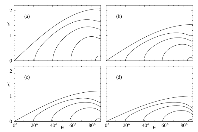
Figure 3: Plots of $\gamma_{1}$ against $\theta$ for type I solutions with $V=4$ and $c$ of $0$ (top curves), $-0.25$, $-0.5$, $-0.75$, and $-0.99$ (lowest curves). (a) $b=0$ (b) $b=2$ (c) $b=4$ (d) $b=50$.

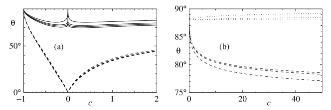
Figure 4: Plots of $\theta_{\rm max}$ [solid lines], $\theta_{\rm crit}$ [dashed lines], and $\theta_{\rm c}$ [dotted lines] against $c$: (a) $V=4$ with $b$ taking the values $0$ (top curves), $2$, $4$, and $50$ (lowest curves); (b) $V=-4$ with $b$ taking the values $5$ (outermost curves), $10$, and $20$ (innermost curves).

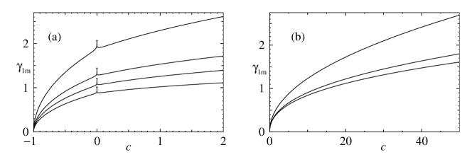
Figure 5: Plots of $\gamma_{\rm 1m}$ against $c$: (a) $V=4$ with $b$ taking the values $0$ (top curves), $2$, $4$, and $50$ (lowest curves) – dots indicate value of $\gamma_{1}$ calculated for solitary wave solutions in Part 1; (b) $V=-4$ with $b$ taking the values $5$ (top curves), $10$, and $20$ (lowest curves).

In Part 1 it was found that $\gamma_{1}$ for solitary waves decreases with increasing $b$ for a fixed value of $\eta$. As is apparent from equation (2.2) of Part 1, for fixed $\eta$, the amplitude decreases as $b$ increases. However, if the amplitude is fixed (by using the appropriate value of $\eta$ in each case) then it is found that $\gamma_{1}$ increases with $b$. Cnoidal waves for different values of $b$ but with the same amplitude and values of $m$ will have different periods. It therefore seems inappropriate to compare the growth rates in such cases. Nevertheless, meaningful comparisons can be made on examining the entire growth rate curve as a function of $\theta$. As can be seen from Figs. 3 and 5(a), there is a more marked variation of the growth rate with $\theta$ for angles above $\theta_{\rm max}$ as $b$ increases, and the plots in Fig. 4(a) indicate that $\theta_{\rm max}$ deviates from the perpendicular most of all when $b$ is large. On the other hand, $\theta_{\rm crit}$ shows only a slight dependence on $b$.

We now turn to the stability results for solutions in the form of functions extended by periodicity. When $V>0$ and $c$ is increased above zero, one obtains type II_pe solutions. It can be seen from Fig. 6(a)-(c) that the first-order growth rates of these solutions are higher than that for the soliton limit at some angles, but this range of angles decreases with increasing $b$. In addition to an increasing $\theta_{\rm crit}$ with $c$, the first-order growth rate for exactly perpendicular perturbations vanishes for large enough $b$ and $c$. Evidently the growth rate has a significantly greater angular dependence than for the Type I solutions.

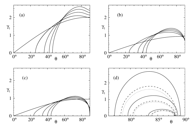
Figure 6: Plots of $\gamma_{1}$ against $\theta$ for type II_pe and I_pe solutions. In (a)-(c), $V=4$ and $c$ takes the values $0$ (leftmost curves), $0.5$, $1.0$, $1.5$ and $2.0$ (rightmost curves) and (a) $b=0$ (b) $b=4$ (c) $b=50$. In (d) $V=-4$ and $c$ takes the values $50$ (top curves), $10$, and $1$ (lowest curves) with $b=5$ [solid lines], $b=10$ [dashed lines], and $b=20$ [dotted lines].

For the stability results we have examined so far, the first-order growth rate is non-zero for angles just below 90^∘. In the case of type I_pe and II_pe solutions when $V<0$ the results in Fig. 6(d) indicate that there is a cut-off angle $\theta_{\rm c}$ above which $\gamma_{1}$ vanishes. Hence such waves are, to first order, stable to perpendicular perturbations. In addition, the instability occurs over a relatively small range of angles, even for large values of $c$. For these types of solution, as is shown in Fig. 5(b), the growth rate increases monotonically with $c$, in contrast to the behaviour near the type I to type II_pe transition. There is no spike in the growth rate at $c=1$, the type I_pe-II_pe transition, since there is no sudden change of period around that point.

5 Conclusions

This article has dealt with the small-$k$ stability with respect to transverse perturbations of cnoidal wave solutions to the SKdVZK equation which governs strongly magnetized plasma with slightly non-isothermal electrons. It was found that the growth rate of instabilities for ordinary cnoidal waves that travel faster than long-wavelength linear waves has a stronger angular variation as the distribution of electrons becomes increasingly flatter than the isothermal Maxwellian. We also examined a class of solutions that do not occur for equations without a square root term. These solutions, which are written as functions extended by periodicity, have a minimum value of zero. This causes difficulties with some instances of recursion relations used in the determination of the growth rate, and results in it being necessary to evaluate an additional integral. This type of solution, for the case when the wave velocity is less than that of long-wavelength linear waves, has, to first order, a relatively narrow range of perturbation angles at which instability occurs and is stable to perpendicular perturbations.

The half-integer nonlinear term in the SKdVZK equation was originally introduced by Schamel to model the effect of trapped particles in Bernstein-Greene-Kruskal (BGK) solutions of the Vlasov-Poisson equation. Hence Part 1 and this paper are to be viewed as a step towards the more formidable problem of studying the stability of the BGK modes where trapped particles play a significant role.

Appendix A The evaluation of $\alpha_{1/2}$, $\alpha_{1}$ and $\alpha_{3/2}$

For cnoidal wave solutions, $\alpha_{1/2}$, $\alpha_{1}$, and $\alpha_{3/2}$ are elliptic integrals and for their evaluation we therefore rely heavily on Byrd and Friedman (1954) to which the result numbers in the following refer.

Type I solutions

The type I solution as given by (2.6) has a period of $2K(m)/\eta$ where $K(m)$ is the complete elliptic integral of the first kind. From result 340.01 we obtain

$$\alpha_{1/2}=r_{1}+(r_{4}-r_{1})\frac{\Pi(-\rho|m)}{K(m)}$$ (A.38)

in which $\Pi(n|m)$ is the complete elliptic integral of the third kind.

Applying result 340.02 to (2.6) yields

$$\alpha_{1} = \frac{(r_{4}-r_{1})^{2}}{2(\rho+1)(1+m)}\left(\frac{\rho E(m)+\{\rho^{2}+2\rho(1+m)+3m\}\Pi(-\rho|m)}{K(m)}-\rho-m\right)$$ (A.39)

$$\mbox{}+r_{1}^{2}+2r_{1}(r_{4}-r_{1})\frac{\Pi(-\rho|m)}{K(m)}$$

where $E(m)$ is the complete elliptic integral of the second kind.

Type II_pe solutions

After introducing

$$\sigma=\frac{A-B}{A+B},\qquad\sigma_{1}=\frac{Ar_{\rm l}-Br_{\rm u}}{Ar_{\rm l}+Br_{\rm u}},\qquad\bar{I}_{n}=\int_{0}^{\bar{\chi}}\!\!\frac{\,{\rm d}X}{(1-\sigma\mathop{\mathrm{cn}}\nolimits(X|\bar{m}))^{n}},$$

the integrals $\alpha_{n/2}$ for $n=1,2,3$ may be written in the form

$$\alpha_{n/2}=\frac{1}{\bar{\chi}}\left(\frac{Ar_{\rm l}-Br_{\rm u}}{A-B}\right)^{n}\sum_{p=0}^{n}\left(\begin{array}[]{c}n\\ p\end{array}\right)(\sigma/\sigma_{1}-1)^{p}\bar{I}_{p}.$$

From results 341,

$$\bar{I}_{1}=\frac{1}{1-\sigma^{2}}\left(\Pi(-q;\bar{\phi}|\bar{m})+\frac{\sigma}{\mu}\tan^{-1}[\mu\mathop{\mathrm{sd}}\nolimits(\bar{\chi}|\bar{m})]\right)$$ (A.40)

where $q=\sigma^{2}/(1-\sigma^{2})$, $\bar{\phi}=\mathop{\mathrm{am}}\nolimits(\bar{\chi}|\bar{m})$, $\mu=\sqrt{\bar{m}+q}$, $\mathop{\mathrm{sd}}\nolimits(x|m)\equiv\mathop{\mathrm{sn}}\nolimits(x|m)/\mathop{\mathrm{dn}}\nolimits(x|m)$,

$$\bar{I}_{2}=\frac{\{2\bar{m}-(2\bar{m}-1)\sigma^{2}\}\bar{I}_{1}+\sigma^{2}E(\bar{\phi}|\bar{m})-\{\bar{m}+(1-\bar{m})\sigma^{2}\}\bar{\chi}+\bar{\Upsilon}_{1}}{(1-\sigma^{2})\{\bar{m}+(1-\bar{m})\sigma^{2}\}},$$

$$\bar{I}_{3}=\frac{3\{2\bar{m}-(2\bar{m}-1)\sigma^{2}\}\bar{I}_{2}+2\bar{m}F(\bar{\phi}|\bar{m})-\{6\bar{m}-(2\bar{m}-1)\sigma^{2}\}\bar{I}_{1}+\bar{\Upsilon}_{2}}{2(1-\sigma^{2})\{\bar{m}+(1-\bar{m})\sigma^{2}\}},$$

where $F(\phi|m)$ is the elliptic integral of the first kind, and

$$\bar{\Upsilon}_{n}=\frac{\sigma^{3}\mathop{\mathrm{sn}}\nolimits(\bar{\chi}|\bar{m})\mathop{\mathrm{dn}}\nolimits(\bar{\chi}|\bar{m})}{(1-\sigma\mathop{\mathrm{cn}}\nolimits(\bar{\chi}|\bar{m}))^{n-1}}.$$

Type I_pe solutions

The $\alpha_{n/2}$ for $n=1,2,3$ may be written in the form

$$\alpha_{n/2}=\frac{\displaystyle{r_{1}^{n}}}{\displaystyle{\chi}}\sum_{p=0}^{n}\left(\begin{array}[]{c}n\\ p\end{array}\right)\left(r_{4}/r_{1}-1\right)^{p}I_{p},$$

where

$$I_{n}=\int_{0}^{\chi}\!\!\frac{\,{\rm d}X}{(1+\rho\mathop{\mathrm{sn}}\nolimits^{2}(X|m))^{n}}.$$

From result 400.01, $I_{1}=\Pi(-\rho;\phi|m)$, where $\phi=\mathop{\mathrm{am}}\nolimits(\chi|m)$. Results 336.01 and 336.02 yield

$$I_{2}=\frac{\sigma E(\phi|m)-(m+\rho)\chi+\{2\rho(1+m)+3m+\rho^{2}\}I_{1}+\Upsilon_{1}}{2(1+\rho)(m+\rho)},$$ (A.41)

$$I_{3}=\frac{mF(\phi|m)-2\{\rho(1+m)+3m\}I_{1}+3\{2\rho(1+m)+3m+\rho^{2}\}I_{2}+\Upsilon_{2}}{4(1+\rho)(m+\rho)},$$ (A.42)

respectively, where

$$\Upsilon_{n}=\frac{\rho^{2}\mathop{\mathrm{sn}}\nolimits(\chi|m)\mathop{\mathrm{cn}}\nolimits(\chi|m)\mathop{\mathrm{dn}}\nolimits(\chi|m)}{(1+\rho\mathop{\mathrm{sn}}\nolimits^{2}(\chi|m))^{n}}.$$

References

- Allen et al. (2007) Allen, M. A., Phibanchon, S. and Rowlands, G. 2007 J. Plasma Phys. (in press, available online).
- Byrd and Friedman (1954) Byrd, P. F. and Friedman, M. D. 1954 Handbook of Elliptic Integrals for Engineers and Physicists. Berlin: Springer-Verlag.
- Infeld (1985) Infeld, E. 1985 J. Plasma Phys. 33, 171.
- Infeld and Rowlands (2000) Infeld, E. and Rowlands, G. 2000 Nonlinear Waves, Solitons and Chaos, 2nd edn. Cambridge: Cambridge University Press.
- Munro and Parkes (1999) Munro, S. and Parkes, E. J. 1999 J. Plasma Phys. 62, 305.
- O’Keir (1993) O’Keir, I. S. 1993 The Stability of Solutions to Modified Generalized Korteweg-de Vries, Nonlinear Schrödinger and Kadomtsev-Petviashvili Equations Ph.D. Thesis, University of Strathclyde.
- O’Keir and Parkes (1997) O’Keir, I. S. and Parkes, E. J. 1997 Physica Scripta 55, 135.
- Parkes (1993) Parkes, E. J. 1993 J. Phys. A: Math. Gen. 26, 6469.
- Phibanchon (2006) Phibanchon, S. 2006 Nonlinear Waves in Plasmas with Trapped Electrons Ph.D. Thesis, Mahidol University.
- Rowlands (1969) Rowlands, G. 1969 J. Plasma Phys. 3, 567.
- Schamel (1972) Schamel, H. 1972 Plasma Phys. 14, 905.
- Schamel (1973) Schamel, H. 1973 J. Plasma Phys. 9, 377.
- Zemanian (1965) Zemanian, A. H. 1965 Distribution Theory and Transform Analysis. New York: McGraw-Hill.