A non local shell model of turbulent dynamo
Abstract
We derive a new shell model of magnetohydrodynamic (MHD) turbulence in which the energy transfers are not necessary local. Like the original MHD equations, the model conserves the total energy, magnetic helicity, cross-helicity and volume in phase space (Liouville’s theorem) apart from the effects of external forcing, viscous dissipation and magnetic diffusion. In the absence of magnetic field the model exhibits a statistically stationary kinetic energy solution with a Kolmogorov spectrum. The dynamo action from a seed magnetic field by the turbulent flow and the non linear interactions are studied for a wide range of magnetic Prandtl numbers in both kinematic and dynamic cases. The non locality of the energy transfers are clearly identified.
pacs:
47.65.+a1 Introduction
Pioneering shell models of hydrodynamic turbulence were developed in the seventies [1, 2, 3, 4, 5], aiming at reproducing the main turbulence features, as intermittency, with a low order model of equations. Such shell models were also called wave packet representation [6] for the Fourier space is logarithmically divided into shells of logarithmic width such that each wave packet (or shell) is defined by . Those models are local in the sense that each shell interacts with only the first neighbours like the DN model (named after Desnyansky and Novikov [4]), or the two first neighbours like the GOY model (named after Gledzer, Ohkitani and Yamada [3, 7]). The latter has been intensively studied (for a review, see [8, 9, 10, 11] and references therein) and subjected to improvements leading to the so-called Sabra model [12, 13, 14] or extensions using the wavelet decomposition [15]. The GOY and subsequently Sabra models have been used in different contexts like convection [16], rotation [17] or intermittency [18, 19]. It has been shown [20] that the DN model is a spectral reduction of the GOY model, showing in some sense the consistency of one model against the other.
To our knowledge only one non-local shell model of turbulence has been developed so far, by Zimin and Hussain [21], projecting the Navier-Stokes equations onto a wavelet basis, and reducing the number of variables from statistical assumptions. In such non-local model each shell may interact with any other shell. Since then, the original model has been improved by Zimin in order to include left- or right-handed polarity of the solenoidal basis functions as in the complex helical wave decomposition, and used by Melander and Fabijonas [22, 23, 24].
The extension of shell models to MHD turbulence has been done including either first neighbours interactions [25, 26, 27, 28] or two first neighbours interactions [29, 30, 31, 32, 33] eventually including Hall effect [34, 35]. However there is a number of situations in MHD turbulence in which assuming the locality of energy transfers may become somewhat spurious even if the turbulence is considered as isotropic [33]. This is true for example when a large scale external magnetic field is imposed leading to Alfven waves [36, 37, 38]. This problem has been tackled using a MHD shell model implementing non local interactions with the externally imposed magnetic field scale [28]. However it has been shown recently using an other method [39] that the other non local interactions are also important and may rule out the predicted Iroshnikov-Kraichnan spectrum. Non local interactions are also at the heart of the dynamo problem i.e. when the magnetic field is produced by the turbulent motion instead of being externally applied. For example at large value of the magnetic Prandtl number, the magnetic spectrum is observed to peak at scales much smaller than the viscous scale [40, 41, 42] showing a direct evidence of the importance of non local energy transfers. In presence of helicity, two possible mechanisms may generate a large scale magnetic field as observed in planets and stars: either a local inverse cascade [43] or a non local direct transfer from small to large scales as predicted by the mean-field theory [44]. Which mechanism prevails is still not clear. Recently, the importance of non-local interactions has been shown in both hydrodynamic [45] and MHD [46, 47, 48] turbulence. For recent reviews on MHD turbulence and the dynamo problem, see e.g. [49, 50]
In the present paper our aim is to introduce a new non local shell model of turbulence which can be used either in its hydrodynamic or MHD form. As we are interested by MHD applications, we shall introduce the MHD model only, the hydrodynamic one being easily deduced from the former, setting the magnetic field to zero. Our model can be understood as a non local version of the Sabra model. This involves similar rules for complex conjugations and imposes the value of shell spacing equal to the golden number. Our first attempt to derive a non local shell model of MHD turbulence was based on the Zimin model [21]. However we realized that this model was unable to describe the non local interaction between a large scale velocity and two small neighboring scales of the magnetic field. We believe that the one which is described here is more relevant to actual isotropic MHD turbulence.
2 General concept
2.1 The model
The model is defined by the following set of equations
| (1) | |||||
| (2) |
where
| (3) |
represents the non linear transfer rates. The parameters and are respectively the kinematic viscosity and the magnetic diffusivity, is the forcing of turbulence, and with [12]. For in (3), we recognize the local Sabra model. The additional non local interactions for correspond to all other possible triad interactions except the ones involving two identical scales. Expressions for the kinetic energy and helicity , magnetic energy and helicity , and cross helicity are given by
| (4) | |||||
| (6) | |||||
In the inviscid and non-resistive limit (), the total energy , magnetic helicity and cross helicity must be conserved (). This leads to the following expression for the coefficients and :
| (7) |
In the case of pure hydrodynamic turbulence (without magnetic field), the coefficients are derived from the kinetic energy and helicity conservations (), leading again to the same expression as (7). The coefficients are free parameters depending on only, that we choose of the form . The coefficient is chosen such that the terms for in correspond to the local Sabra model. The local Sabra model corresponds to .
2.2 All possible interactions
In our shell model we see from (3) that only a discrete number of triads are allowed. For example, does not contain any term involving interactions between the modes and . The reason why there is only a discrete number of allowed triads comes from the fact that the shells are logarithmically spaced and that the geometrical factor satisfies
| (8) |
To identify all the allowed triads in a shell model, let us consider three vectors satisfying
| (9) |
Assuming that and belong to shell and , we have
| (10) |
From (9), this implies
| (11) |
Now using the inequalities (8) and (11) we can show that belongs to shell which depends on in the following way:
|
(12) |
This is illustrated in Figure 1 in the plane where the grey (resp. white) squares indicate allowed (resp. not allowed) triads (). The demonstration of (12) is given in Appendix A. In Figure 1, the terms corresponding to the original Sabra local model are denoted by “L”, the additional non local terms by “N” and the terms of Zimin’s model by “Z”. In every case the possible shells are symmetric with respect to the diagonal in the plane .
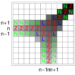 |
|
2.3 Evaluation of
There is one free parameter left, , which corresponds to the non locality
strength. It is not an easy task (if possible at all) to figure out what should be in the general case.
However we tried to estimate it in the case of homogeneous isotropic turbulence (without
magnetic field). For that,
we take two random
vectors from shell , and
uniformly distributed in whole space, and
we calculate the probability that and belong respectively to shells and . It is the simplest estimate of the probability that the three modes , and interact together. A high (resp. low) value of this probability
is given in Figure 1 by the dark (resp. light) colour of the grey squares. In this representation a white square
correspond to a null probability.
The probability spectra along the
and directions
are found to scale as
for the ”L” and ”N” terms
and
for the ”Z” terms (which is consistent
with the Zimin’s model [21]).
In order to have terms and in (3) scaling in ,
we have to take . We note that this derivation of does not imply the terms (and neither the diagonal terms of Figure 1). The latters are determined a posteriori from the conservation laws (not included in the probability diagram of Figure 1).
In section 3.1.1 we shall find that the value is the most appropriate to describe accurately the large scale slope of the kinetic energy spectrum. However,
in the rest of the paper we shall vary the value of in order to investigate the
role of in the non local interactions.
2.4 Energy transfers
To study the non local interactions, we introduce the transfer rate from -energy lying in shell to -energy lying in shell . It can operate only within triads, implying an additional energy lying in all other shells different from and . Denoting the transfer rate from to and which involves as a mediator, the transfer rate from to can then be written as
| (13) |
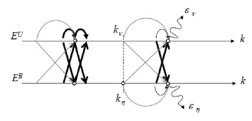
From our model (3) we see that for each couple , only a discrete number of can act as mediators. The possible triads are represented schematically in Figure 2.
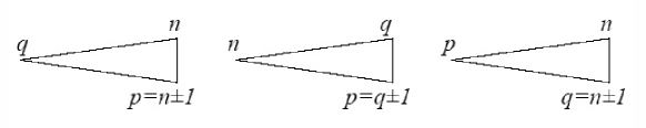
(a) (b) (c)
Therefore takes the following form
| (14) |
Now, we have to define for any , and . For that, we can re-write the model (1) (2) in the following generic form
| (15) |
where is a symmetric bilinear form (given in Appendix B) representing the quadratic terms. The dots represent the dissipation and forcing terms appropriate to .
Now let us denote by the rate of energy within the triads which is transferred from the couple to . It is naturally defined by
| (16) |
As is symmetric, we have
| (17) |
In addition,and with the help of (7), we can show that for any triad the following relation is satisfied
| (18) |
meaning that the energy is conserved within each triad.
Then we look for as a linear combination of , and .
As in real MHD turbulence, must satisfy the following conditions
| (19) | |||||
| (20) |
The first condition (19) means that the transfer rate from to and from to with the same mediator are of equal intensity but opposite signs. We note that this implies
| (21) |
The second condition (20) means that in any triad the transfer rate from to is equal to the sum of the transfer rates from to via and from to via . Then combining (17),(18), (19) and (20) we end up with the following expression for
| (22) |
Furthermore we can show that the following energy balances at scale are satisfied
| (23) | |||||
| (24) |
with the kinetic and magnetic dissipation rates in shell defined by
| (25) |
and
| (26) |
2.5 Energy fluxes
We define the energy flux as the rate of loss of -energy lying in the shells to the -energy lying in the shell . Therefore, we have
| (27) | |||||
| (28) |
The fluxes and coincide respectively with and . There is no such coincidence for and .
The following flux balances are satisfied
| (29) | |||
| (30) |
In a statistically stationary case they imply that
| (31) |
In order to investigate the importance of non local versus local interactions, we define the local part of the fluxes given by (27) in which only the local energy transfer rates , and are involved. These fluxes correspond to those of the MHD version of the original (local) Sabra model, taking in (3). The non local parts of the fluxes are defined as the total fluxes minus their local parts.
2.6 Hydrodynamic forcing
The hydrodynamic forcing is generally applied at scale and with . It is of the form where is constant during time intervals , the constant value changing randomly from one time interval to the next one. In this way we obtain a statistically constant injection rate equal to . We chose for it is smaller than the turn-over time at the injection scale and larger than the viscous characteristic time.
For some arbitrary initial conditions on of small intensity we let the hydrodynamic evolve until it reaches some statistically stationary state. Then introducing at a given time some small intensity of we solve the full problem until a statistically stationary MHD state is reached. The time of integration needed to obtain good statistics depends on and but is typically of several hundreds of time unit (of the largest scale ). We define the magnetic Prandtl number as the ratio .
To study the free decaying turbulence, after having reached a statistically stationary state, the forcing is set to zero.
3 Results
3.1 Energy spectra
3.1.1 Free decaying turbulence
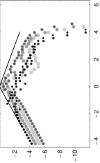
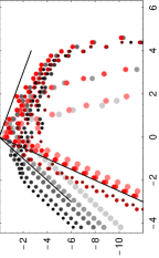
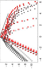
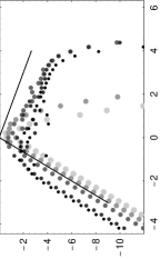
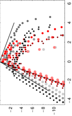
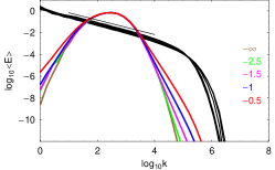
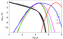
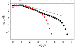
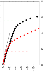
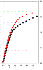
In this section we study free decaying turbulence without and with magnetic field. The results are presented in Figure 3 for , different values of and . The kinetic (magnetic) spectra are plotted with grey (red) dots at different times. The initial conditions are such that the cross-helicity is close to zero at any scale. Trying the same simulation but with an initial condition with a cross-helicity equal to 1 leads to inertial ranges poorly defined. The time sample at which the spectra are plotted is . The dots corresponding to are the darkest and the smallest.
We observe that changing does not change the slope of the inertial range for both kinetic and magnetic spectra. This slope compares well with the Kolmogorov slope ( in spectral space) which is represented by the straight line with negative slope in each plot. In the other hand, changing changes drastically the slope at large scale. The kinetic and magnetic energy slopes are indicated by the two straight lines with positive slopes in each plot.
In table 1 these slopes are indicated for both spectra and for the different values of that are considered.
| -2.5 | -1.5 | -1 | -0.5 | ||
|---|---|---|---|---|---|
| Kinetic slope | 10 | 5 | 3 | 2 | 1 |
| Magnetic slope | 12 | 7 | 5 | 4 | 3 |
From hydrodynamic turbulence theory, a slope in ( in spectral space) is expected at large scales. The only value of which gives such slope is . The slope for the local Sabra model, corresponding here to , leads to a slope in ( in spectral space) much larger than the one predicted by the theory. This is a first drastic difference between the local and non local models which emphasizes the importance of including the non local interactions.
We note that there is always a difference of 2 between the magnetic and kinetic slopes, leading to a magnetic spectrum slope in ( in spectral space) for . Though seems to be the most appropriate for hydrodynamic and MHD turbulence, in the rest of the paper we shall investigate other values of as well, in order to investigate the role of in non local transfers.
|
|
|
|
|
||
|---|---|---|---|---|---|
|
|
 |
 |
 |
 |
|
|
|
 |
 |
 |
 |
|
|
|
 |
 |
 |
 |
|
|
|
 |
 |
 |
 |
|
|
|
 |
 |
 |
 |
|
3.1.2 Forced turbulence
In forced turbulence we consider shells larger than 0 (). We could also have considered a cut-off at any other arbitrary negative shells. However, in order to reach a stationary state it is important to have a cut off scale above which the system is not solved (like some integral scale or the scale of the box in an experiment). Considering negative shells without limit would imply energy to fill all shells on a time scale of the order and without reaching a stationary state.
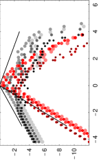
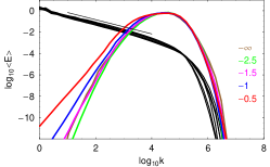
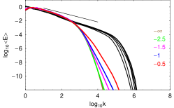
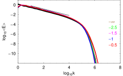
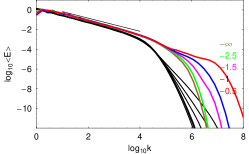
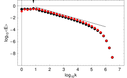
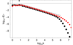
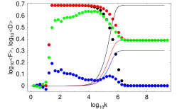
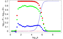
In Figure 4 both kinetic and magnetic energy spectra are plotted for three values of
and both kinematic and saturated dynamo regimes. In each plot, the curves correspond to different values of . In the kinematic regime (top plots) the Lorentz forces corresponding to the term are small and can be neglected in the energy balance. Then the magnetic energy grows exponentially at any scale. In Figure 4 the magnetic spectra are normalized by the maximum value of .
In the saturated regime (bottom plots), the Lorentz forces act back onto the flow, leading to statistically stationary kinetic and magnetic energies.
In both kinematic and dynamic regimes and for (left and middle plots of Figure 4),
the effect of is not really significant.
The kinetic spectra (black curves) are almost not sensitive to non local interactions showing that hydrodynamic interactions are mostly local as predicted by the Kolmogorov cascade. Besides the kinetic spectra always scale as ( in the spectral space) in the inertial range.
We see some non local effects onto the magnetic spectra
(colour curves) which spread towards large scales or even small scales for .
However, the scale for which
the spectrum is maximum does not change and is roughly equal to as again predicted by Kolmogorov arguments (see e.g. [33]).
In the other hand, the non local effect are much more significant for (plots on the right), mainly for the magnetic spectra at scales smaller than the viscous scales () and for . In the kinematic regime the maximum of the magnetic energy spectrum occurs at scales smaller than when . In the dynamic regime some magnetic bottle neck appears. To understand why it is so, let us first recall that the flow scale which produces magnetic field in the most efficient way is the one for which the shear is the largest [33]. In the inertial range the flow shear scales as , and it is then maximum for . Therefore the non local interactions relevant for the magnetic spectrum extension towards smaller scales are mostly those involving . The non local terms involving and generating magnetic energy with involves also . The corresponding non local term in (2) are in the form which scale as . Therefore we understand that for the non local effect may be strong at small scales.
 |
 |
 |
Kinematic |
 |
 |
 |
Dynamic |
3.2 Energy fluxes
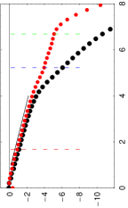
In this section we set and and consider the dynamo saturated regime for three values of and . The kinetic and magnetic spectra are plotted in the top row of figure 5. Both spectra have inertial ranges of Kolmogorov types, scaling in (scaling in in the spectral space). For we identify clearly that the magnetic dissipation scale is much smaller than the viscous dissipation scale. However the distinction between them is not so clear for .
 |
 |
 |
Spectra |
 |
 |
 |
Fluxes |
 |
 |
 |
Non local fluxes |
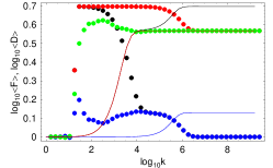
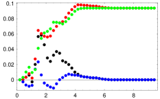
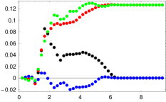
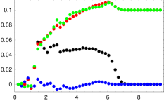
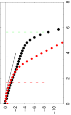
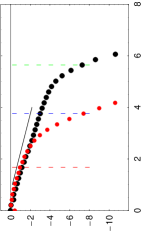
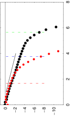
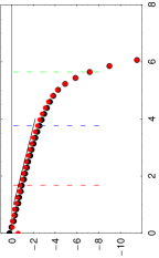
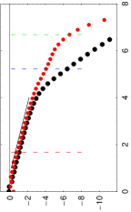
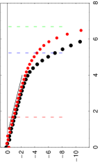
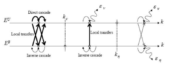
The total and non local part of the fluxes are plotted in middle and bottom rows of figure 5. The non local part of is found to be always much smaller than , implying that the energy transfers are mainly local. In the other hand, the importance of the non local part of versus the local one depends on .
In figure 6 the ratio is plotted for the three values of . For this ratio is about 20 %. For and for scales smaller than the viscous scale , this ratio increases up to 50%. Finally, for there is a discontinuity at , the ratio being then equal to -100% at smaller scales. These are first evidences of non local interactions.

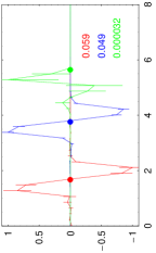
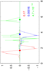
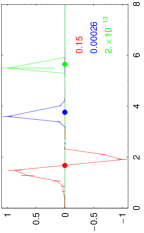
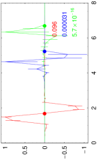
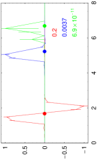
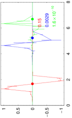
3.3 Energy transfers
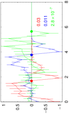
The four energy transfers are plotted in Appendix C in figures 8,
9 and 10 for respectively and .
In each figure the column from left to right corresponds to and . The row from second to bottom corresponds to
the transfer , , and .
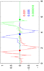
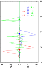
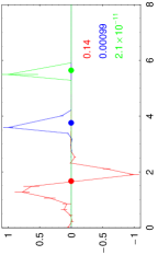
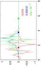
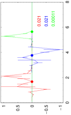
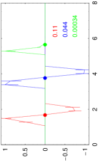
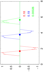
The transfers are plotted versus , for three values of which are indicated
by the dashed vertical lines on the spectra plots on top row and by the red, green or blue dots. The transfers being time-dependent we plot their time-average with error bars corresponding to the standard deviation of the mean. This gives some estimation of the robustness of the results. Some quantities are much more noisy than the others and then less reliable.
The local transfers seem to be always dominant whatever the values of or .
However there are also some evidence of non local transfers which are discussed below.
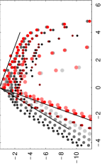
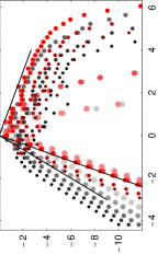
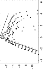
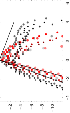
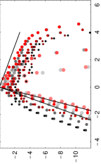
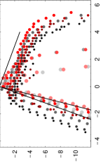
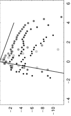
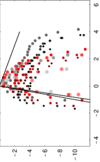
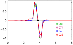
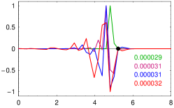
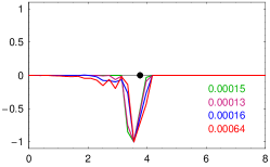
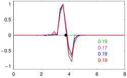
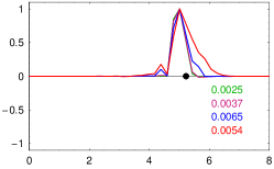
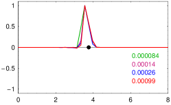
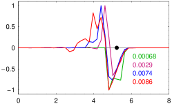
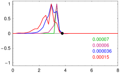
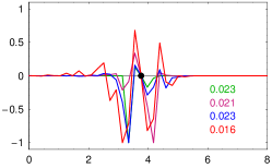
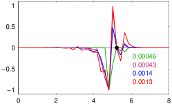
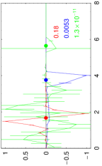
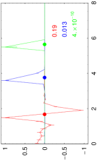
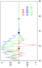
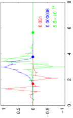
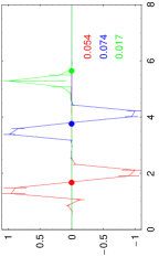
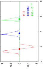
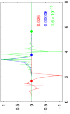
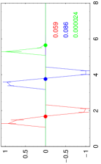
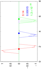
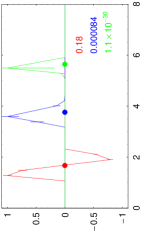
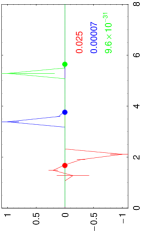
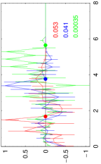
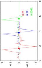
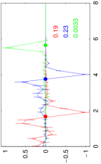
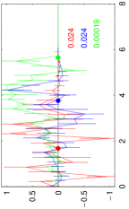
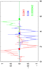
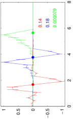
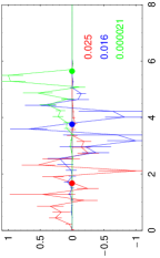
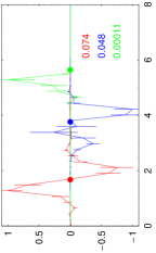
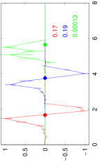
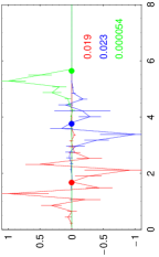
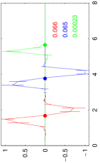
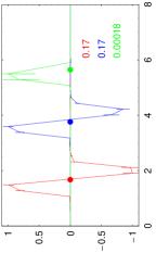
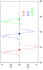
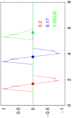
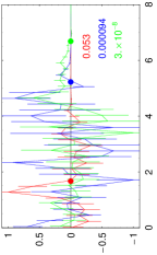
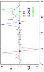
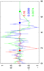
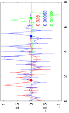
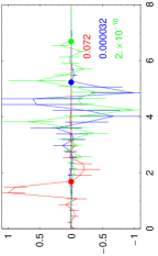
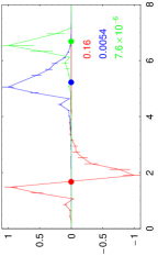
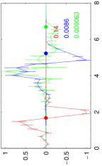
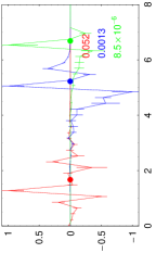
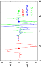
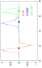
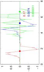
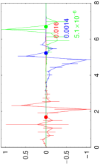
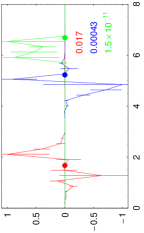
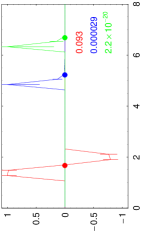
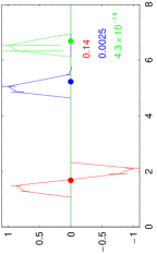
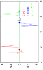
In figure 7 some typical results are presented for the three values of and (from left to right column), each row from top to bottom corresponding to the transfers , , and for one given value of denoted by the black dot. The curves correspond to (green), (magenta), (blue) and (red).
-
•
For , , implying that the dominant energy transfer which feeds the kinetic energy is a local direct cascade of kinetic energy.
-
•
For and , implying that the kinetic energy is mainly obtained from magnetic field. This transfer is found to be mainly local.
-
•
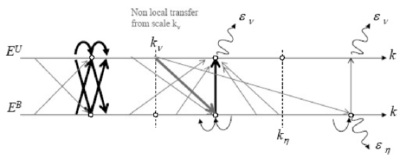
For we find that is mainly local and always negative. It means that energy is transferred locally from to (which is consistent with the curve just below). In addition, we see that the curve of extends towards larger and larger scales when goes to zero. Though it is small (up to 20%), it is a clear evidence of non local transfer from small scale kinetic to large scale magnetic energy. We interpret it as an alpha-effect in the sense of mean field theory.
-
•
The curves of for show also clear evidence of non local transfers. In this case, is fed by scales of much larger than . There is also some local transfer back from to shown by the curves of .
-
•
For and though much smaller than , there is clear evidence of non local direct cascade of magnetic energy as shown by .
-
•
Finally, for and , shows evidence of some kind of non local inverse cascade though much smaller than .
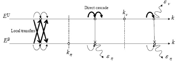
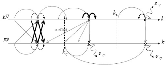
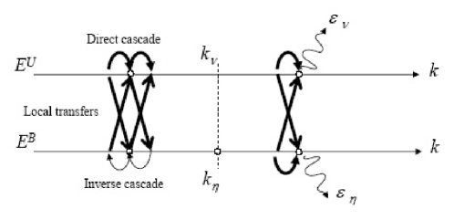
In figures 11, 12 and 13 of Appendix D we give some qualitative illustration of the previous interpretation of the results.
 |
 |
 |
|
 |
 |
 |
|
 |
 |
 |
|
 |
 |
 |
|
4 Discussion
The main originality of the shell model presented in (2)(3) is that it
takes into account all possible non local interactions between different shells.
In essence it is a non local MHD version of the Sabra model.
Deriving the model we find that there is one free parameter that we call
(and which is different from the alpha-effect of the mean-field dynamo theory).
In some sense this parameter controls the strength of non locality of the model.
An estimation of has been done on the basis of simple probabilistic arguments of
possible triad interactions, leading to .
However, in free decaying hydrodynamic turbulence, we find numerically that the value gives the right slope of the kinetic spectrum at large scales ( as predicted by the turbulence theory in spectral space). Therefore seems the most appropriate value for hydrodynamic turbulence.
In comparison we note that the local Sabra model (corresponding here to ) leads to a slope
about .
In the other hand, in MHD turbulence it is not obvious that has to be the same as in hydrodynamic turbulence. Actually, it is even not obvious that should not depend from the scale , which is not possible in our model. Therefore we investigated several values of ranging several values from to zero. Several values of have been investigated depending if it is lower than, equal to or larger than 1.
In order to characterize the non local energy transfers from to within any possible triad, the quantities have been derived an plotted versus for a few values of . Though most of them are local, several energy transfers have been found to be partially non local, depending on .
Appendix A Possible triads in logarithmic shell models
For a given shell , we first take benefit from the fact that the triads () and () are identical and then the representation in the plane is symmetric with respect to the diagonal. We then limit our demonstration to half of (12):
- •
- •
- •
- •
- •
Appendix B Expressions of the energy transfers
Appendix C Energy transfers results
|
Spectra |
|
|
|
|
||
|---|---|---|---|---|---|---|
|
|
 |
 |
 |
 |
 |
|
|
|
 |
 |
 |
 |
 |
|
|
|
 |
 |
 |
 |
 |
|
|
|
 |
 |
 |
 |
 |
|
|
|
 |
 |
 |
 |
 |
|
|
Spectra |
|
|
|
|
||
|---|---|---|---|---|---|---|
|
|
 |
 |
 |
 |
 |
|
|
|
 |
 |
 |
 |
 |
|
|
|
 |
 |
 |
 |
 |
|
|
|
 |
 |
 |
 |
 |
|
|
|
 |
 |
 |
 |
 |
|
|
Spectra |
|
|
|
|
||
|---|---|---|---|---|---|---|
|
|
 |
 |
 |
 |
 |
|
|
|
 |
 |
 |
 |
 |
|
|
|
 |
 |
 |
 |
 |
|
|
|
 |
 |
 |
 |
 |
|
|
|
 |
 |
 |
 |
 |
|
Appendix D Illustration of the energy transfers
 |
 |
 |
 |
 |
 |
References
References
- [1] A.M. Obukhov. Some general characteristic equations of the dynamics of the atmosphere. Atmos. Oceanic Phys., 7:41, 1971.
- [2] E. Lorenz. Low order models representing realizations of turbulence. J. Fluid Mech., 55:545, 1972.
- [3] E.B. Gledzer. System of hydrodynamic type admitting two quadratic integrals of motion. Dokl. Akad. Nauk. SSSR, 209:1046, 1973. [Sov. Phys. Dokl. 18, 216 (1973)].
- [4] V.N. Desnyansky and E.A. Novikov. The evolution of turbulence spectra to the similarity regime. Izv. Akad. Nauk. SSSR Fiz. Atmos. Okeana, 10:127, 1974.
- [5] E.D. Siggia. Origin of intermittency in fully developed turbulence. Phys. Rev. A, 15:1730, 1977.
- [6] T. Nakano. Direct interaction approximation of turbulence in the wave packet representation. Phys. Fluids, 31:1420, 1988.
- [7] M. Yamada and K. Ohkitani. Lyapunov spectrum of a chaotic model of three-dimensional turbulence. J. Phys. Soc. Jpn., 56:4210, 1987.
- [8] U. Frisch. Turbulence: The Legacy of A.N. Kolmogorov. Cambridge Univ. Press, 1995.
- [9] T. Bohr, M.H. Jensen, G. Paladin, and A. Vulpiani. Dynamical Systems Approach to Turbulence. Cambridge Univ. Press, 1998.
- [10] S.B. Pope. Turbulent flows. Cambridge Univ. Press, 2000.
- [11] L. Biferale. Shell models of energy cascade in turbulence. Ann. Rev. Fluid Mech., 35:441–468, 2003.
- [12] V. L’vov, E. Podivilov, A. Pomlyalov, I. Procaccia, and D. Vandembroucq. Improved shell model of turbulence. Phys. Rev. E, 58:1811, 1998.
- [13] V. L’vov, E. Podivilov, and I. Procaccia. Hamiltonian structure of the sabra shell model of turbulence: Exact calculation of an anomalous scaling exponent. EurPhys. Lett., 46:609, 1999.
- [14] P.D. Ditlevsen. Symmetries, invariants, and cascades in a shell model of turbulence. Phys. Rev. E, 62:484, 2000.
- [15] R. Benzi, L. Biferale, R. Tripiccione, and E. Trovatore. (1+1)-dimensional turbulence. Phys. Fluids, 9:2335–63, 1996.
- [16] J. Mingshun and L. Shida. Scaling behavior of velocity and temperature in a shell model for thermal convective turbulence. Phys. Rev. E, 56:441, 1997.
- [17] Y. Hattori, R. Rubinstein, and A. Ishizawa. Shell model for rotating turbulence. Phys. Rev. E, 70:046311, 2004.
- [18] M.H. Jensen, G. Paladin, and A. Vulpiani. Intermittency in a cascade model for three-dimensional turbulence. Phys. Rev. A, 43:798, 1991.
- [19] D. Pierotti. Intermittency in the large-n limit of a spherical shell model for turbulence. Europhys. Lett., 37:323–328, 1997.
- [20] J.C. Bowman, B. Eckhardt, and J. Davoudi. Spectral reduction of the goy shell turbulence model. http://www.math.ualberta.ca/ bowman/talks/caims04.pdf, 2004.
- [21] V. Zimin and F. Hussain. Wavelet based model for small-scale turbulence. Phys. FLuids, 7:2925, 1995.
- [22] M. Melander. Helicity causes chaos in a shell model of turbulence. Phys. Rev. Lett., 78:1456, 1997.
- [23] M. Melander and B. Fabijonas. Self similar enstrophy divergence in a shell model of isotropic turbulence. J. Fluid Mech., 463:241, 2002.
- [24] M. Melander and B. Fabijonas. Transients in the decay of isotropic turbulence. J. Turb., 4:014, 2003.
- [25] R. Grappin, J. Léorat, and A. Pouquet. Computation of the dimension of a model of fully developed turbulence. J. Phys. (France), 47:1127, 1986.
- [26] C. Gloaguen, J. Léorat, A. Pouquet, and R. Grappin. A scalar model for mhd turbulence. Physica D, 51:154, 1985.
- [27] V. Carbone. Scale similarity of the velocity structure functions in fully developed magnetohydrodynamic turbulence. Phys. Rev. E, 50:671, 1994. [Eurphys. Lett. 27, 581 (1994)].
- [28] D. Biskamp. Cascade models for magnetohydrodynamic turbulence. Phys. Rev. E, 50:2702, 1994.
- [29] P. Frik. Hierarchical model of two-dimensional turbulence. Magn. Gidrodin., 19:60, 1983. [Magnetohydrodynamics 19, 48 (1983)].
- [30] P. Frik. Two-dimensional mhd turbulence. hierarchical model. Magn. Gidrodin., 20:48, 1984. [Magnetohydrodynamics 20, 262 (1983)].
- [31] A. Brandenburg, K. Enquist, and P. Olesen. Large-scale magnetic fields from hydromagnetic turbulence in the very early universe. Phys. Rev. D, 54:1291, 1996.
- [32] P. Frick and D. Sokoloff. Cascade and dynamo action in a shell model of magnetohydrodynamic turbulence. Phys. Rev. E, 57:4155, 1998.
- [33] R. Stepanov and F. Plunian. Fully developed turbulent dynamo at low magnetic prandtl number. Journ. Turb., 7:39, 2006.
- [34] D. Hori, M. Furukawa, S. Ohsaki, and Z. Yoshida. A shell model for the hall mhd system. J. Plasma Fusion Res., 81:141–142, 2005.
- [35] P. Frick, R. Stepanov, and V. Nekrasov. Shell model of the magnetic field evolution under hall effect. Magnetohydrodynamics, 39:327–334, 2002.
- [36] R. H. Kraichnan. Inertial-range spectrum of hydromagnetic turbulence. Phys. Fluids, 8:1385, 1965.
- [37] R.H. Kraichnan and S. Nagarajan. Growth of turbulent magnetic fields. Phys. Fluids, 10:859, 1967.
- [38] P.S. Iroshnikov. Turbulence of a conducting fluid in a strong magnetic field. Astron. Zh., 40:742, 1963. [Sov. Astron. 7, 566 (1964)].
- [39] M. K. Verma. Mean magnetic field renormalization and kolmogorov’s energy spectrum in magnetohydrodynamic turbulence. Phys. Plasmas, 6:1455–1460, 1999.
- [40] N. E. Haugen, A. Brandenburg, and W. Dobler. Is nonhelical hydromagnetic turbulence peaked at small scales ? Astrophys. J., 597:141–144, 2003.
- [41] A.A. Schekochihin, S.C. Cowley, G.W. Hammett, J.L. Maron, and J.C. McWilliams. A model of nonlinear evolution and saturation of the turbulent mhd dynamo. New J. Phys., 4:84, 2002.
- [42] A.A. Schekochihin, J.L. Maron, S.C. Cowley, and J.C. McWilliams. The small-scale structure of magnetohydrodynamic turbulence with large magnetic prandtl numbers. Atrophys. J., 576:806, 2002.
- [43] A. Pouquet, U. Frisch, and J. Léorat. Strong mhd helical turbulence and the non linear dynamo effect. J. Fluid Mech., 77:321–354, 1976.
- [44] F. Krause and K.-H. Rädler. Mean–Field Magnetohydrodynamics and Dynamo Theory. Pergamon Press, 1980.
- [45] A. Alexakis, P.D. Mininni, and A. Pouquet. Imprint of large-scale flows on turbulence. Phys. Rev. Lett., 95:264503, 2005.
- [46] P.D. Mininni, A. Alexakis, and A. Pouquet. Shell-to-shell energy transfer in magnetohydrodynamics. ii. kinematic dynamo. Phys. Rev. E, 72:46302, 2005.
- [47] A. Alexakis, P.D. Mininni, and A. Pouquet. Shell-to-shell energy transfer in magnetohydrodynamics. i. steady state turbulence. Phys. Rev. E, 72:46301, 2005.
- [48] D. Carati, O. Debliquy, B. Knaepen, B. Teaca, and M. Verma. Energy transfers in forced mhd turbulence. Journ. Turb., 7:1–12, 2006.
- [49] M. K. Verma. Statistical theory of magnetohydrodynamic turbulence: recent results. Phys. Reports, 401:229–380, 2004.
- [50] A. Brandenburg and K. Subramanian. Astrophysical magnetic fields and non linear dynamo theory. Phys. Rep., 417:1–209, 2005.