Electric field dynamics and ion acceleration in the self-channeling of a superintense laser pulse

Abstract

The dynamics of electric field generation and radial acceleration of ions by a laser pulse of relativistic intensity propagating in an underdense plasma has been investigated using an one-dimensional electrostatic, ponderomotive model developed to interpret experimental measurements of electric fields [S. Kar et al, New J. Phys. 9, 402 (2007)]. Ions are spatially focused at the edge of the charge-displacement channel, leading to hydrodynamical breaking, which in turns causes the heating of electrons and an “echo” effect in the electric field. The onset of complete electron depletion in the central region of the channel leads to a smooth transition to a “Coulomb explosion” regime and a saturation of ion acceleration.

1 Introduction

Self-focusing and guiding of laser pulses is one of the most peculiar effects in nonlinear optics. In the case of superintense laser pulses (having irradiances beyond $10^{18}~{}\mbox{Wcm}^{-2}\mu\mbox{m}^{2}$) propagating in a plasma, self-focusing arises due to the combined effects of the intensity dependence of the index of refraction for relativistic electron velocities and of the expulsion of plasma from the propagation axis driven by the radial ponderomotive force [1, 2, 3]; this latter effect leads to self-channeling, i.e. to the creation of a low-density channel that may act as a waveguide for the laser pulse. As the ponderomotive force acts on the plasma electrons, the channel is first drilled in the electron density only and becomes strongly charged [4, 5]; the electric field in the channel leads to ion acceleration [6, 7, 8], which is of interest both as a diagnostic of the interaction and as a way to provide fast ions for applications, e.g. for the production of fusion neutrons [9, 10, 11]. Besides these applications, the self-channeling process may be of relevance for laser-plasma acceleration of electron [12] and ion beams [13, 14], X- and $\gamma$-ray sources [15, 16], and fast ignition in laser-driven Inertial Confinement Fusion [17].

To interpret experimental results on self-channeling and related ion acceleration or neutron production, a simple modeling of the radial dynamics based on the ponderomotive force and electrostatic field only has often been used [18, 8, 6, 7, 10, 19]. Such a ponderomotive, electrostatic model (PEM) is attractive due to its simplicity and easy numerical implementation with respect to multi-dimensional, electromagnetic particle-in-cell (PIC) simulations which typically require massively parallel computing, while simulations based on the PEM in one spatial dimension (1D), taking only the radial dynamics into account, can be performed on a personal computer. Of course the simple PEM gives a strongly simplified description of the interaction where effects such as the nonlinear evolution of the pulse due to self-focusing or instabilities are not included. The use of the PEM can be justified only by its ability to reproduce, at least qualitatively, experimental observations for particular regimes.

Recently, the proton imaging technique [20] allowed for the first time the detection, with spatial and temporal resolution, of the electrostatic, slowly-varying fields produced during and after the self-channeling process (previous experimental investigations [4, 21, 22, 18, 23, 6] were based on optical diagnostics or indirect measurements not directly sensitive to electric fields). The proton imaging data were well reproduced numerically by simulating the proton probe deflection in the space- and time-dependent electric field distribution obtained from PIC simulations based on the 1D PEM. Moreover, a similar dynamics of the electric field and the ion motion in radial direction was also observed in two-dimensional (2D) electromagnetic PIC simulations of the laser-plasma interaction [19, 24].

Motivated by the fair agreement with experimental results and more complex simulations, we have used the PEM to gain an insight of the radial dynamics during and after the self-channeling process. Although there may be much additional physics at play that is not included in the simple PEM, a study based on the latter can be useful to discriminate purely ponderomotive and electrostatic effects from those due to other contributions, e.g. self-generated magnetic fields [22], anisotropy and polarization effects [25], hosing instabilities [26, 27], and so on.

It turns out that the dynamics contained in the 1D PEM is already quite rich. We focus our attention on the regime where there is not a complete depletion of electrons in the channel and the electric field almost exactly balances the ponderomotive force (PF) locally. From the point of view of ion acceleration we call this the “ponderomotive” regime, since the force on ions is proportional to the PF, while we call “Coulomb explosion” the regime in which, due to complete electron depletion, the ions move under the action of their own space-charge field only. Our analysis shows that the transition between the two regimes occurs rather smoothly.

A prominent effect observed in the simulation is the spatial “focusing” of the ions at the edge of the channel, where they form a very sharp spike of the ion density. The density spike splits up rapidly due to hydrodynamical breaking, and a short bunch of “fast” ions is generated. Density spiking and breaking occur even for pulse durations shorter than the time needed for ions to reach the breaking point. The onset of hydrodynamical breaking also causes a strong heating of electrons and the formation of an ambipolar sheath field around the breaking point. For pulse durations shorter than the time at which breaking occurs, there is a sort of “echo” effect in the electric field, which vanishes at the end of the laser pulse to re-appear later at the breaking location. Simple analytical descriptions of the spatial focusing mechanism and of the ambipolar field structure around the density spike are given. Finally, the smooth transition toward the “Coulomb explosion” regime is described both analytically and via simulations.

2 The model

We now give a detailed description of the 1D, electrostatic, ponderomotive model which has been already used in Ref.[19] to simulate the radial electron and ion dynamics due to self-channeling of an intense laser pulse in an underdense plasma. Only the slowly-varying dynamics of the plasma electrons is taken into account, i.e. a temporal average over oscillations at the laser frequency is assumed. In other words, what we describe is the dynamics of electron “guiding centers”, i.e. of quasi-particles moving under the action of the ponderomotive force (PF). The PF associated to a laser pulse described by the vector potential ${\bf A}({\bf x},t)$ can be written, under suitable conditions (see e.g. [28]), as

$${\bf F}_{p}({\bf x},t) = -m_{e}c^{2}\mbox{\boldmath$\nabla$}\gamma({\bf x},t),$$ (1)

$$\gamma({\bf x},t) = \left[1+\langle{\bf a}^{2}({\bf x},t)\rangle\right],$$ (2)

$${\bf a}({\bf x},t) = (e/m_{e}c^{2}){\bf A}({\bf x},t),$$ (3)

where the angular brackets denote average over a period. We assume a non-evolving laser pulse (neglecting pulse diffraction, self-focusing and energy depletion) and complete cylindrical symmetry around the propagation axis, taking only the radial dynamics into account. Under such simplifying assumptions, the laser pulse is completely defined by the cycle-averaged squared modulus of the vector potential in dimensionless units, which we write as

$$a^{2}(r,t)=\langle{\bf a}^{2}({\bf x},t)\rangle=a^{2}(r){\cal P}(t)=a^{2}_{0}e^{-r^{2}/r_{0}^{2}}{\cal P}(t).$$ (4)

where ${\cal P}(t)$ is the temporal envelope. The radial component of the PF can thus be written as

$$F_{r} = F_{r}(r,t)=-m_{e}c^{2}\partial_{r}\gamma,$$ (5)

$$\gamma = \gamma(r,t)=\left[{1+{a^{2}(r,t)}}\right]^{1/2}.$$ (6)

Unless $a_{0}\ll 1$ the electron dynamics is relativistic. For $a_{0}\gtrsim 1$, besides using the relativistic expression of the PF one has to account for the inertia due to the high-frequency quiver motion. This is included via an effective, position-dependent mass $m=m_{e}\gamma$ of the quasi-particles [28]. We thus write for the radial momentum

$$p_{e,r}\simeq m_{e}\gamma v_{r}.$$ (7)

Therefore, the equation of motion for the electrons is written as

$$\frac{dp_{e,r}}{dt}=F_{r}-eE_{r}$$ (8)

where $E_{r}$ is the electrostatic field due to the space-charge displacement. The effect of the laser force on ions having mass $m_{i}=Am_{p}\gg m_{e}$ can be neglected, leaving the electrostatic force $ZeE_{r}$ as the only force on the ions. The ion equation of motion is thus written as

$$\frac{dv_{i}}{dt}=\frac{Z}{A}\frac{e}{m_{p}}E_{r}.$$ (9)

The electrostatic field is computed via Poisson’s equation

$$\partial_{r}E_{r}=4\pi e(Zn_{i}-n_{e}).$$ (10)

Equations (8), (9) and (10) are the basis of our particle simulations in 1D cylindrical geometry.

Thanks to the low dimensionality of our model, it is possible to use a very high resolution in the simulations. A typical run used $40000$ spatial gridpoints, with a spatial resolution $\Delta r=d_{p}/500$ where $d_{p}=c/\omega_{p}$ is the plasma frequency, and up to $3\times 10^{7}$ particles for both electron and ion distributions. It turned out that such a high resolution is needed to resolve the very sharp spatial structures that are generated during the simulation, as it will be discussed below. The initial temperature of the plasma is taken to be zero and no significant numerical self-heating is observed during the simulations.

In the simulation results shown below, the spatial coordinate $r$ is normalized to the laser wavelength $\lambda$, the time to the laser period $T_{L}$, the density to the critical density $n_{c}$, and the electric field to the “relativistic” threshold field $E_{0}$. The definition of these parameters and their value in “practical” units for the typical choice $\lambda=1~{}\mu\mbox{m}$ are as follows:

$$T_{L} = \frac{\lambda}{c}=3.34\times 10^{-15}~{}\mbox{s},$$ (11)

$$n_{c} = \frac{m_{e}c^{2}}{\pi e^{2}\lambda^{2}}=1.11\times 10^{21}~{}\mbox{cm}^{-3},$$ (12)

$$E_{0} = 2\pi\frac{m_{e}c^{2}}{e\lambda}=3.21\times 10^{10}~{}\mbox{V cm}^{-1}.$$ (13)

Momenta are given in units of $m_{i}c$ for ions and $m_{e}c$ for electrons, respectively.

To compare with experiments, we note that the pulse intensity as a function of time and position is given by

$$I(r,t)=\frac{\pi c}{\lambda^{2}}\left\langle A^{2}(r,t)\right\rangle=\pi\left(\frac{m_{e}c^{2}}{e\lambda}\right)^{2}a^{2}(r,t).$$ (14)

The relation

$$a_{0}=0.85\times\left(\frac{I_{0}\lambda^{2}}{10^{18}~{}\mbox{W cm}^{-2}\mu\mbox{m}^{2}}\right)^{1/2}$$ (15)

thus gives the parameter $a_{0}$ as a function of the maximum intensity $I_{0}$, i.e. as the value of the intensity at the center of the laser spot and at the pulse peak. Some care should be taken when comparing to experiments where some average value, i.e. the pulse energy over the spot area and the pulse duration, is given instead; inserting such an average value into Eq.(15) would represent too low a value for a proper comparison.

The “pulse duration” and “spot radius” quoted in experimental papers most of the times refer to the FWHM of the temporal envelope and to half the FWHM of the radial profile of the intensity, respectively. In our model the laser pulse intensity varies as

$${\cal P}(t)=\sin^{4}\left(\frac{\pi t}{\tau}\right)=\sin^{4}\left(\frac{1.14t}{\tau_{1/2}}\right).$$ (16)

for $0<t<\tau$, while ${\cal P}(t)=0$ for $t>\tau$. (A Gaussian pulse envelope has also been tested, but no significant differences in the simulation results was evidenced.) The parameter $\tau_{1/2}=1.14\tau/\pi$ is thus the FWHM duration of the laser pulse intensity. For the Gaussian radial profile, the FWHM radius of the intensity profile is $r_{1/2}=\sqrt{\ln 2}r_{0}\simeq 0.83r_{0}$.

3 Results

The particle code based on the PEM was developed to analyze the experiment of Ref.[19], and the most relevant results emerged during such analysis. Therefore the first simulation we show, which gives us the basis for our discussion, has been performed for laser and plasma parameters in the range of those covered by the experiment of Ref.[19]. In the latter, the laser pulse wavelength was $\lambda=1.053~{}\mu\mbox{m}$, the intensity was in the range from $4\times 10^{18}$ to $2\times 10^{19}~{}\mbox{W cm}^{-2}$, the duration was $\tau_{1/2}\simeq 1.2~{}\mbox{ps}\simeq 330~{}T_{L}$ and the waist radius in vacuum was $r_{1/2}\simeq 5~{}\lambda$. As the effective values of the pulse amplitude and radius may change during the propagation into the plasma, the values of $a_{0}$ and $r_{0}$ were varied in the simulation until the best match in the reconstruction of proton images was found [19]. The plasma was created in a gas jet of Helium (charge state $Z=2$, mass number $A=4$) and the typical electron density $n_{e}$ was in the range from $10^{18}$ to $10^{19}~{}\mbox{cm}^{-3}$, i.e from about $10^{-2}n_{c}$ to $10^{-1}n_{c}$.

3.1 Ion dynamics and hydrodynamical breaking

Fig.1 shows the spatial profiles of the electric field $E_{r}$ and of the ion density $n_{i}$, and the distribution functions in the ($r,p_{r}$) phase space of ions ($f_{i}$) and electrons ($f_{e}$) at four different times, which are representative of the subsequent stages of the dynamics. Fig.2 shows the complete space–time evolution of $E_{r}$ and $n_{i}$ from the same simulation as contour plots. The parameters are $a_{0}=2.7$, $n_{e}/n_{c}=0.01$, $r_{0}=7.5\lambda$, $\tau_{1/2}=330T_{L}$.

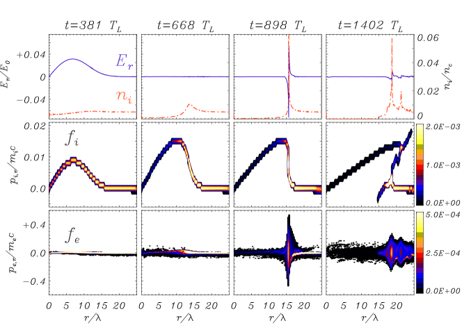
Figure 1: (color online) Simulation results in the ponderomotive regime. The profiles of electric field $E_{r}$ (blue, thick line) and ion density $n_{i}$ (red, dash-dotted line), and the phase space distributions of ions $f_{i}(r,p_{r})$ and electrons $f_{e}(r,p_{r})$ are shown at four instants (with times given in units of the laser period $T_{L}$) which are representative of subsequent stages of the dynamics: the initial ponderomotive acceleration ($t=381T_{L}$), the vanishing of $E_{r}$ after the end of the laser pulse ($t=668T_{L}$), the spiking of $n_{i}$ preceding the hydrodynamical breaking and the rebirth (“echo”) of $E_{r}$ correlated with strong electron heating ($t=898T_{L}$), and the “x” structure of the ion phase space after breaking ($t=1402T_{L}$). Parameters are $a_{0}=2.7$, $n_{e}/n_{c}=10^{-2}$, $r_{0}=7.5\lambda$, $\tau_{1/2}=330T$.

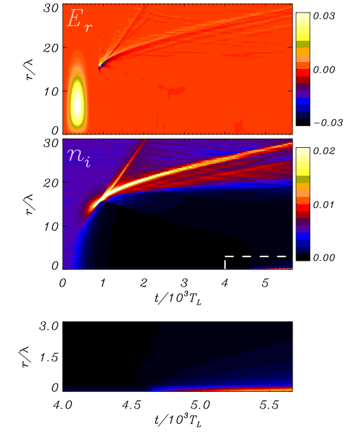
Figure 2: (color online) Space-time contour plots of $E_{r}(r,t)$ (top frame) and $n_{i}(r,t)$ (middle frame) from the same simulation of Fig.1. The bottom frame shows enlarged view of the region marked by the dashed contour in the middle frame, showing the accumulation of ions on the axis at late times. The contour levels have been partly saturated to make regions of low field or density appear.

The dynamics observed in the simulation of Fig.1 can be described as follows. During the laser pulse ($t<\tau$), the PF $F_{r}$ pushes the electrons outwards, quickly creating a positively charged channel along the axis. This charge displacement creates a radial ES field $E_{r}$ which holds the electrons back, as shown in the first frame of Fig.1 for $t=381T_{L}$ (i.e. $\simeq 50$ periods after the pulse peak). In this stage, we find the ES field to balance almost exactly the PF, i.e. $eE_{r}\simeq F_{r}$ (when plotting $F_{r}/e$ as well in Fig.1 for $t=381$, its profile cannot be distinguished from that of $E_{r}$). Thus, at any time the electrons are approximately in a state of mechanical equilibrium. From the electron phase space at $t=381T_{L}$ we also observe that no significant electron heating occurs, $f_{e}$ being a narrow function along the $p_{e,r}$ axis. During this stage the ions are accelerated by the electric force $ZeE_{r}=ZF_{r}$, and a depression in $n_{i}$ is thus produced around the axis. After the end of the pulse ($t\simeq 668T_{L}$ in Fig.1), ion acceleration is over, the peak momentum of the ions is $0.015m_{i}c$, and $E_{r}\simeq 0$. This indicates that the electrons have rearranged their spatial distribution in order to restore the local charge neutrality. At the same time, we still observe a very weak heating of electrons, consistently with the keeping of the mechanical quasi-equilibrium condition up to this stage.

However, the ions retain the velocity acquired during the acceleration stage. For $r>r_{\mbox{\tiny max}}$, where $r_{\mbox{\tiny max}}\simeq r_{0}$ is the position of the PF maximum, the force on the ions decrease with $r$, and thus the ion final velocity does as well. As a consequence the ions starting at a position $r_{i}(0)>r_{\mbox{\tiny max}}$ are ballistically focused towards a narrow region at the edge of the intensity profile. This spatial focusing effect is actually very tight, as in Fig.1 we observe a large number of ions to reach approximately the same position ($r=r_{b}\simeq 15.5~{}\lambda$) at the same time ($t=t_{b}\simeq 898T_{L}$). Here the ions pile up producing a very sharp peak of $n_{i}$. The peak value of $n_{i}$ is $\simeq 46n_{0}=0.23n_{c}$ at $t=898T_{L}$, as shown in the detail of the density and field profiles of Fig.3. The density peak is well out of scale of the density axis in the plots of Fig.1. Simple modeling (see A) provides an estimate of the position $r_{b}$ and the instant $t_{b}$ at which the density spike is formed as a function of the laser pulse parameters:

$$r_{b}\simeq\left(\frac{3}{2}\right)^{3/2}r_{0}\simeq 1.84r_{0},$$ (17)

$$t_{b}\simeq\frac{\pi}{2}e^{3/4}\sqrt{\frac{A}{Z}\frac{m_{p}}{m_{e}}}\frac{r_{0}}{a_{0}c}\simeq 10^{2}T_{L}\sqrt{\frac{A}{Z}}\frac{r_{0}}{a_{0}\lambda}.$$ (18)

The latter expression is likely to be an underestimate for $t_{b}$ as the simple model assumes the pulse intensity to be constant during the time the ions take to reach the point $r=r_{b}$, while in the simulation the pulse is shorter than $t_{b}$ and the value of the amplitude averaged over the pulse duration is lower than $a_{0}$. For the run of Fig.1 we obtain $r_{b}\simeq 14\lambda$ and $t_{b}\simeq 569~{}T_{L}$, in fair agreement with the simulation results.

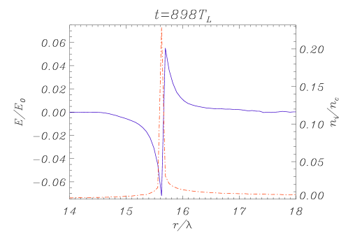
Figure 3: (color online) Detail of the profiles of electric field $E_{r}$ (blue, thick line) and ion density $n_{i}$ (red, dash-dotted line) around the “breaking” point at $t=898T_{L}$, for the simulation of Figs.1 and 2. The peak value of $n_{i}$ exceeds forty times the background value $n_{0}=0.005n_{c}$.

The piling up of ions at the point $r=r_{b}$ leads to hydrodynamical breaking in the ion density profile, as the fastest ions overturn the slowest ones at $r=r_{b}$. The onset of hydrodynamical breaking is clearly evident in the contours of $f_{i}$ at the “breaking” time $t_{b}\simeq 898T_{L}$ (where the typical “vertical” shape of the contours of $f_{i}$ can be noticed). At later times ($t=1402T_{L}$) the ion phase space plot is reminiscent of the so-called “x-type” breaking that was first observed in the collapse of ion acoustic waves excited by Brillouin scattering [29]; in Ref.[2] the occurrence of this type of breaking at the walls of a self-focusing channel was also mentioned, but not discussed in detail.

The ion density breaking leads to the generation of a short ion bunch (located near $r=22\lambda$ at $t=1407T_{L}$), propagating in the outward direction, containing nearly monoenergetic ions having $p_{i}\simeq 0.014m_{i}c$ for the parameters of Figs.1–2. The motion of the bunch is almost purely ballistic, as it is evident in Fig.2.

A similar feature was observed in the case of “longitudinal” ponderomotive acceleration described in Ref.[30], where the bunch formation is also shown to be related to spatial focusing of ions and hydrodynamical breaking of the ion density. In the case investigated in Ref.[30] ion acceleration is also of ponderomotive nature because the use of circularly polarized light prevents the generation of “fast” electrons and thus the onset of sheath ion acceleration.

In addition to the ion bunch, we observe both a small fraction of the ions which is further accelerated at breaking (up to $\simeq 0.014m_{i}c$), and another fraction which is accelerated inwards, having negative $p_{i}$ up to $\simeq-0.005m_{i}c$, and thus moves back towards the axis. At later times ($t\gtrsim 4000T_{L}$) these ions are found to form a local density maximum (i.e. a narrow plasma filament) around $r=0$, as highlighted in Fig.2. A local density maximum on the channel axis was also found in 3D electromagnetic simulations [22] but explained by magnetic pinching, which is absent in our model.

The dynamics of the ions after breaking and related features, such as the “fast” ion bunch and the local density maximum on axis are related to the effect of the generation of a strong ambipolar field at the breaking point, which we now discuss.

3.2 Electric “echo” effect and electron heating

In the electric field plot at the breaking time we observe a strong ambipolar electric field appearing around the breaking point. The field is rather intense (its amplitude slightly exceeding that of the positive field due to charge depletion at earlier times) and highly transient; the complete “movie” of $E_{r}(r,t)$ in Fig.2 shows that the field near the breaking point rises sharply from zero to its peak value over a few laser cycles time, and then decreases less rapidly to lower values (see the profile at $t=1402T_{L}$). The ambipolar structure slowly moves in the outward direction and is observable up to very long times. The “inversion” of the field, i.e. the appearance of a region where the electric fields points towards the axis, in the direction opposite to the initial stage of electron depletion, was evident in the proton imaging measurements reported in Ref.[19]. The electric “echo” is evidently correlated with the rapid and strong heating of electrons at breaking, which we observe in the $f_{e}$ plots at the breaking time.

Figure 4: Electron energy distribution at $r=15.8\lambda$ and $t=898T_{L}$ for the simulation of Figs.1. The dotted line is a two-temperature Maxwellian with $T_{1}=4\times 10^{-3}m_{e}c^{2}$ and $T_{2}=2.5\times 10^{-2}m_{e}c^{2}$.

The generation of an electric field around the density peak as the ions approach the breaking point is interpreted as due to the inability of electrons to dynamically screen the ion field when the density variation is too fast. Let $d$ be the width of the ion peak at a certain time. The density changes in time due to the ballistic motion of ions moving towards the breaking point $r=r_{b}$. The typical variation time of the ion density is $\tau_{i}\sim d/v_{i}$, where $v_{i}$ is the ion velocity determined by the acceleration stage. Electrons respond on a typical time of the order of the inverse plasma frequency, $t_{p}\sim 2\pi/\omega_{p}$, thus they are able to preserve plasma neutrality if ${d}/{v_{i}}>t_{p}$. If such condition is violated, the field around the density spike will be close to the unscreened field of the ions, i.e. a surface field of amplitude $E_{i}\sim\pm 2\pi Zen_{i}d$, leading to electron heating. The “neutrality condition” can be written in terms of the typical units used in the paper as

$$\frac{(d/\lambda)}{(v_{i}/c)}\gtrsim\frac{2\pi}{\omega_{p}}={T_{L}}\sqrt{\frac{n_{c}}{n_{e}}},$$ (19)

which is useful to check its violation in the simulation results. However, it is noticeable that as a function of time $d=d(t)$ may be not independent from the density $n_{e}=n_{e}(t)$; due to mass conservation we expect $d\sim 1/n_{i}$ and thus $d\sim 1/n_{e}$ as far as $n_{e}\simeq n_{i}$ locally. Thus, as $n_{e}$ spikes the l.h.s. of Eq.(19) decreases more rapidly than the r.h.s., boosting the violation of the inequality. This effect might account for the “robustness” of the electric “echo” effect in our simulations. The correlation between the formation of the density spike and electron heating might also be qualitatively understood on the basis of more general arguments, such as the fact that small oscillations of electrons around their point of (quasi–)equilibrium tend to become nonlinear across a sharp density gradient, i.e. around the spike, and lead to heating.

The electron energy distribution $f_{e}$ near the breaking point at $t=898T_{L}$ (Fig.4) for the simulation of of Figs.1 may be roughly approximated by a two–temperatures Maxwellian with values $T_{1}\simeq 4\times 10^{-3}m_{e}c^{2}\simeq 2~{}\mbox{keV}$ and $T_{2}\simeq 2.5\times 10^{-2}m_{e}c^{2}\simeq 12.8~{}\mbox{keV}$. The value of $T_{1}$ is fairly consistent with an electron acceleration in the unscreened ion field leading to typical energies $\sim eE_{i}d$; in fact, estimating $E_{i}\simeq 0.05E_{0}$ and $d\simeq 0.1\lambda$ from Fig.3 we obtain a typical energy $eE_{i}d\simeq 5\times 10^{-3}m_{e}c^{2}$. The presence of the “hot” tail in $f_{e}$ may be a signature of stochastic processes able to accelerate a minor fraction of electrons to higher energies of the order of $T_{2}$.

The electron “temperature” generated during the highly transient heating stage accounts for the persistence of an ambipolar field around the density peak at later times. The almost Maxwellian shape of the electron energy distribution function allows to describe the late electric field as a “Debye sheath” field generated around a thin foil of cold ions and thermal electrons in Boltzmann equilibrium. In such a model the foil is “thin” if the spatial extension (FWHM) of the sheath field, $\ell_{s}$, is larger than the extension of the density “cusp” $d$, which is indeed the case in Fig.3 where $\ell_{s}\simeq 0.3\lambda>d\simeq 0.1\lambda$. The model is analytically solvable in planar geometry (see B) for a delta–like foil density, which is appropriate in the limit $d\ll\lambda_{\mbox{\tiny D}}$ where $\lambda_{\mbox{\tiny D}}$ is the Debye length. Using this analytical result for a rough estimate, we write the peak field $E_{s}$ and the sheath extension $\ell_{s}$ as

$$E_{s}=2\pi en_{i}d,\qquad\ell_{s}=2\frac{4\lambda_{\mbox{\tiny D}}^{2}}{d},$$ (20)

where $n_{i}$ is the ion density in the foil. Assuming parameters values from the 1D simulations, $n_{f}\simeq 0.23n_{c}$, $d\simeq 0.1\lambda$, we find in normalized units $E_{s}/E_{0}=\pi(n_{f}/n_{c})(d/\lambda)\simeq 0.07$, fairly consistent with the simulation results. However, using $T_{e}=T_{1}\simeq 4\times 10^{-3}m_{e}c^{2}$, we obtain $\lambda_{\mbox{\tiny D}}^{2}/d=(T_{e}/m_{e}c^{2})(n_{c}/n_{f})(\lambda^{2}/4\pi^{2}d)\simeq 4.3\times 10^{-3}\lambda$ and thus $\ell_{s}/\lambda\simeq 0.034$, which is smaller than the observed value and not consistent with the assumption $\ell_{s}>d$. This suggests that the sheath is mostly formed by the “hot” electrons having temperature $T_{2}\simeq 6T_{1}$ and lower density (roughly estimated to be $n_{h}\simeq 0.17n_{f}$ from the double–Maxwellian fit of the electron distribution), so that the effective values of $\lambda_{D}^{2}$ and $\ell_{s}$ may increase by one order of magnitude. Replacing $n_{f}$ by $n_{h}$ accounts for the screening by the colder electrons of the ion field acting on the “hot” ones. Due to these effects and additional ones (e.g. the dependence of the sheath profile on the cut-off energy for “truncated” Maxwellians, see B) the simple thin sheath model cannot accurately describe the field around the density spike, but it is at least useful for a qualitative description.

For clarity it is worth to point out that the breaking of the ion fluid and the formation of a strong ambipolar field around the breaking point occurs also for longer pulses, i.e. when the PF and the related electric field are not over at the breaking time. This has been observed by varying the pulse duration in our simulations. The electric field “echo” occurring when the pulse is already over is a remarkable signature of the strong electron heating that occurs following the ion fluid breaking in a regime of plasma neutrality. On a qualitative basis, a possible explanation of the electron heating is that near breaking the temporal variation of the plasma density becomes faster and a very strong density gradient is generated, so that electron oscillations around their equilibrium positions may become non-adiabatic, leading to heating.

The generation of the strong ambipolar field structure, creating a very sharp field gradient at the breaking point, has a feedback effect on the ion distribution, acting as a sort of “axe” that separates slower ions from faster ones. Slower ions are reflected by the negative part of the field and acquire negative radial velocity, thus driving the formation of the density maximum at $r=0$ at $t>1700$ in Fig.2. Faster ions have enough energy to cross the electric field barrier, producing the escaping bunch, and may also receive additional energy from the positive part of the field; this accounts for the ions which are observed to get further momentum after breaking in Fig.1 at $t=1402T_{L}$. These two ions components produce the upper right and lower left “arms” in the x-structure of the phase space at breaking. As the electric field decreases very rapidly after breaking, the other ions form a dense front moving in radial direction with a velocity much smaller than the fast ions in the bunch, as shown in Fig.2. Most of warm electrons remain confined around the ion front and their temperature is found to decrease with time.

3.3 Transition to Coulomb explosion

As stated above, under the action of the PF, the electrons are pushed away from the axis creating a back-holding electrostatic field which balances the PF almost exactly in the ponderomotive regime. However, the balance is possible only if the PF does not exceed the maximum possible value of the electrostatic force at some radius $r$, which occurs if all electrons have been removed up to such value of $r$, i.e. if complete electron depletion occurs, and ions have not moved significantly yet. Within our 1D cylindrical model, an approximate threshold condition for complete electron depletion can be thus derived as follows. If all electrons are removed from a central region and the ion density is equal to its initial value, the electric field in the depletion region is given by

$$E_{d}(r)=2\pi Zen_{i0}r=2\pi en_{e0}r.$$ (21)

If $F_{r}$ exceeds the force due to the “depletion” field $E_{d}(r)$, this will first occur near $r=0$, where $F_{r}$ is given approximately by

$$F_{r}\simeq\frac{m_{e}c^{2}}{r_{0}}\frac{r}{r_{0}}\frac{a_{0}^{2}}{(1+a_{0}^{2})^{1/2}}.$$ (22)

Hence, posing $F_{r}>eE_{d}$ for $r\rightarrow 0$ yields the condition

$$\frac{m_{e}c^{2}}{r_{0}^{2}}\frac{a_{0}^{2}}{(1+a_{0}^{2})^{1/2}}>2\pi e^{2}n_{e0},$$ (23)

which we rewrite as

$$a_{0}>\left[{\frac{k^{2}}{2}+\left({\frac{k^{4}}{4}+k^{2}}\right)^{1/2}}\right]^{1/2},$$ (24)

$$k=2\pi\left(\frac{e^{2}}{m_{e}c^{2}}\right)n_{e}r_{0}^{2}=2\pi r_{c}n_{e}r_{0}^{2},$$ (25)

where $r_{c}=2.82\times 10^{-13}~{}\mbox{cm}$. For $n_{e}=10^{19}~{}\mbox{cm}^{-3}$ ($10^{18}~{}\mbox{cm}^{-3}$) and $r_{0}=7.5~{}\mu\mbox{m}$, we find $k\simeq 10$ ($1$) and thus a complete electron depletion is expected to occur for $a_{0}\gtrsim 10$ [$\gtrsim 1.3$].

The onset of complete electron charge depletion near the axis may occur even lower intensities than predicted by Eq.(24) if the pulse is not too short. In fact, even if initially $F_{r}=eE_{r}$ holds, as the ions move under the action of the force $ZeE_{r}=ZF_{r}$ the density near the axis must decrease, so the maximum electrostatic field that can be generated near the axis also decreases in time, and the condition of complete electron depletion may be met.

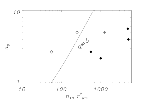
Figure 5: Threshold for the transition from the “ponderomotive” to the “Coulomb explosion” regime. The thick line gives amplitude threshold for complete electron density depletion in the central region [Eq.(24)] as a function of the parameter $n_{e0}r_{0}^{2}$ with $n_{e0}$ in units of $10^{18}~{}\mbox{cm}^{-3}$ and $r_{0}$ in units of $1~{}\mu\mbox{m}$. Filled, empty and “gray” dots represent simulations where the electron depletion is absent, strong, or “marginal”, respectively. The labels $a$ and $b$ indicate two simulation for almost identical parameters but different pulse duration, so that in the longer pulse case ($b$) electron depletion is favored.

Fig.5 shows the threshold amplitude as a function of $n_{e}r_{0}^{2}$. The data points in Fig.5 represent the values of $n_{e}r_{0}^{2}$ for numerical simulations where electron depletion in the central region is either absent (empty, “white” diamonds) or evident (filled, “black” diamonds). With “gray” diamonds we indicate “near–threshold” cases where depletion occurs just very near to the $r=0$ axis and the maximum force on ions is still given by $ZF_{r}$, i.e. the PF is larger than $E_{r}$ over most of the spatial range. The distribution of data points confirm that Eq.(24) gives just a rough condition for the transition from the ponderomotive to the Coulomb explosion regime and that this transition also depends on the pulse duration. For example, the labels a and b in Fig.5 indicate two simulations which have very similar values of $a_{0}$ and $n_{e}r_{0}^{2}$, but for b the electron depletion is much stronger. This can be explained by the pulse duration for case b that is roughly two times the value for case a.

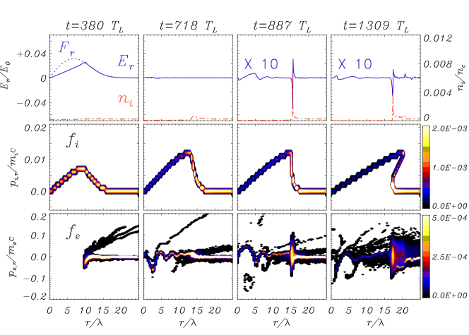
Figure 6: (color online) Simulation results in the regime of strong electron depletion and Coulomb explosion. All the fields and distributions are the same of Fig.1, except that the normalized ponderomotive force $F_{r}/e$ is shown (blue, dotted line) in the leftmost upper plot. The vertical scales for the $E_{r}$ and $p_{i,r}$ (ion momentum) are the same of Fig.1, while to improve readability in the upper two plots for $t=902T_{L}$ and $t=1402T_{L}$, $E_{r}$ has been multiplied by $10$, and the scale for $p_{e,r}$ has been shrunken with respect to Fig.1. Parameters are $a_{0}=2.7$, $n_{e}/n_{c}=10^{-3}$, $r_{0}=7.5\lambda$, $\tau_{1/2}=330T$.

In the Coulomb explosion regime, the ions in the region of electron depletion will be accelerated by their own space charge field. Fig.6 shows results of a 1D simulation where the laser pulse parameters are the same of Fig.1, but the density has been lowered by a factor of 10 (thus, $n_{e}/n_{c}=10^{-3}$). For such parameters, from Eq.(24) we expect to enter the Coulomb explosion regime. The plot of $E_{r}$ and of the scaled PF $F_{r}/e$ in Fig.6 at $t=380T_{L}$ and the corresponding contour plot of $f_{e}$ show that complete charge depletion occurs in the region $r<r_{d}\simeq 8~{}\lambda$. For $r>r_{d}$, $eE_{r}\simeq F_{r}$ still holds. We notice that at the boundary of the depletion layer ($r\simeq r_{d}$), where the force balance breaks down, a few electrons are accelerated to relatively high velocity and escape towards the outer region.

Due to electron depletion the resulting maximum force on the ions $F_{\mbox{\tiny max}}\simeq ZeE_{r}(r_{d})$ is less than the maximum of $ZF_{r}$; thus, the maximum momentum of ions at the end of the laser pulse ($t\simeq 718T_{L}$) is lower than in the case of Fig.1 for the same value of the laser intensity. Hence, for a given laser pulse, ion acceleration saturates for decreasing plasma densities as the condition (24) is crossed. The plots corresponding to the later times show that the spiking and breaking of the ion density, followed by ion bunch formation and ambipolar field generation, still occurs for these parameters; however, both the field amplitude and the electron energy are lower now. In simulations where the electron density is further lowered, electron depletion occurs over almost all the pulse profile, almost all ions are accelerated by the Coulomb explosion, while bunch formation and ambipolar field generation tend to disappear.

3.4 Saturation mechanisms for ion acceleration

In the ponderomotive regime as defined above, the force on the ions is given by $ZeE_{r}=-Zm_{e}c^{2}\partial_{r}[1+a^{2}(r,t)]^{1/2}$. If the temporal dependence of the pulse intensity is neglected, i.e. $a^{2}(r,t)\simeq a^{2}(r)$, one may use the “ponderomotive potential”, $\Phi_{p}(r)=Zm_{e}c^{2}[(1+a^{2}(r))^{1/2}-1]$ to estimate the final energy of ions as a function of their starting position. This assumption leads to a maximum ion energy equal to the peak value of $\Phi_{p}$,

$$U_{i}^{\mbox{\tiny max}}\simeq\Phi_{p}(r=0)\simeq Zm_{e}c^{2}\left[(1+a_{0}^{2})^{1/2}-1\right],$$ (26)

that is the energy acquired by ions initially located on the channel axis, i.e. at $r=0$. In Ref.[8] this relation has been actually used to estimate the peak intensity on axis from the analysis of the ion spectrum.

A clear limitation of this simple picture is the quite long time it would take for an ion starting at $r=0$ to go downhill the ponderomotive potential and to gain the maximum energy, as the PF is very small near $r=0$. Thus, the laser pulse duration may be shorter than the acceleration time, limiting the ion energy. This is indeed the case for the simulation of Fig.1 where the laser pulse is over before the fastest ions have moved out of the radial extension of the pulse. The maximum ion energy observed in Fig.1 is about four times lower than the estimate based on Eq.(26). In this case using the ion energy cut-off to evaluate $a_{0}$ in Eq.(26) would lead to an underestimate of the peak intensity.

As discussed in section 3.3, the possible onset of complete electron depletion is another limiting factor for the ion energy as it gives an an upper limit to the accelerating force. The overall energy spectrum may also be modified by the onset of hydrodynamical breaking at the edge of the beam radius as discussed in sections 3.1 and 3.2.

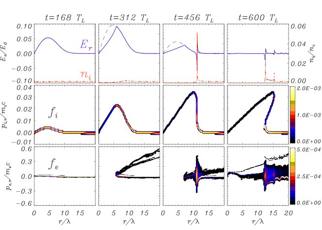
Figure 7: (color online) Simulation results for parameters similar to those of Ref.[8] ($a_{0}=3.5$, $n_{e}/n_{c}=0.01$, $r_{0}=5\lambda$, $\tau_{1/2}=300T$). All the fields and distributions are the same of Figs.1 and 6.

To compare with preceding work we have simulated a case with almost the same parameters as those used in the calculations performed in Ref.[8] to interpret the experimental data. A He plasma is considered and the parameters are $n_{e}/n_{c}=0.01$, $r_{1/2}\simeq 1.2r_{0}=6\lambda$, $\tau_{1/2}=300T$, and $a_{0}=3.5$ [this is lower than the value $a=5$ quoted in Ref.[8] due to a different convention in the expression of the PF, i.e. $F_{r}=(1+a^{2}/2)^{1/2}$]. Simulation results are shown in Fig.7. The maximum ion energy, corresponding to the ions in the “fast” bunch, is $\simeq 2.2~{}\mbox{MeV}$, very close to the energy spectrum cut-off in Fig.2 of Ref.[8], and significantly lower than the $2.7~{}\mbox{MeV}$ value corresponding to Eq.(26). This is due to the complete electron depletion in the central region, occurring about 60 cycles before the pulse peak and keeping the electrical force $eE_{r}$ below the maximum of the PF $F_{r}$, as shown in Fig.7. The breaking of the ion density profile occurs at $r\simeq 11~{}\lambda$, very close to the analytical estimate given by Eq.(30), and at $t\simeq 456T_{L}$, roughly two times the value obtained from Eq.(31).

4 Discussion and conclusions

The one-dimensional electrostatic, ponderomotive model used in this paper to investigate the dynamics of self-channeling yields results whose agreement with experiments is remarkable, taking the simplicity of the model into account. A prominent example has been provided by proton imaging data which have been reproduced by simulating the particle deflection in the electric field computed by the present model [19]. Ion spectra have been also calculated for different laser and plasma parameters and agree with measurements within experimental uncertainties.

Of course one should not forget that the model gives a very simplified description of the laser-plasma interaction, neglecting effects such as pulse diffraction and nonlinear evolution, and so on. The cases in which the simple model is successful in reproducing quantitatively or, at least, qualitatively some features observed in experiments or in more complex and self-consistent simulations, correspond to regimes in which the plasma dynamics during and after the self-channeling of the laser pulse is dominated by ponderomotive and electrostatic forces, other effects playing a secondary role. An example has been provided by the 2D electromagnetic simulations reported in Ref.[24] where the breaking of the channel walls, which has been characterized in detail with the 1D model, causes the formation of two secondary laser beamlets propagating at an angle $\sim\lambda/r_{0}$, consistently with a “leaking waveguide” picture.

The analysis of the simulation results has evidenced details of the dynamics of ion acceleration and electric field generation. In particular, hydrodynamical breaking has been shown to play an important role, causing electron heating, formation of an ambipolar field around the density cusp and, finally, affecting the ion spectrum. Unfolding this dynamics provided an insight on the formation of “x-type” structures in the ion phase space which had been previously observed in different contexts [29]. The related production of a dense, quasi-monoenergetic “bunch” of ions revealed similarities with the process of ponderomotive acceleration of ions in overdense plasmas [30]. A prominent consequence of hydrodynamical breaking, occurring for pulse durations shorter than the breaking time, is the “echo” observed in the electric field, i.e. its sudden rebirth after having disappeared at the end of the laser pulse.

Throughout our work we found useful to distinguish the regime of “ponderomotive acceleration” from that of “Coulomb explosion”. In the first case, complete depletion of the electron density does not occur, the ponderomotive and the electric forces balance almost exactly and electrons are in a state close to mechanical equilibrium at all times before breaking; in such a regime the ponderomotive potential can be used to estimate the ion energy given the laser intensity (or vice versa), although the effects of finite pulse duration must be considered. In the second case, electron density depletion occur near the axis and the ions in this region are accelerated by their own space-charge field, leading to a saturation of the peak ion energy versus the laser intensity. An approximate analytical criterion for the transition between the two regimes have been given and tested by simulations, which also shows that such transition occurs smoothly.

Appendix A Analytical estimate of breaking point location

A simple model can be used to account for the spatial focusing effect and estimate its characteristic parameters (i.e. the position and the instant at which the density spike is formed). For the sake of simplicity, let us neglect the temporal variation of $F_{r}$. If $F_{r}$ was a linear function of $r$, the ion equation of motion would be of the harmonic oscillator type,

$$m_{i}\frac{d^{2}r_{i}}{dt^{2}}=ZF_{r}\simeq-k(r_{i}-r_{b}),$$ (27)

implying that all the ions starting from an arbitrary radius $r_{i}(0)<r_{b}$ would get to $r=r_{b}$ at the time $t_{b}=(2\pi/\Omega)/4$, where $\Omega\equiv\sqrt{k/m_{i}}$. In our case $F_{r}$ is not a linear function of $r$, but a linear approximation of $F_{r}$ is quite accurate around the point $r=r_{f}$ such that $\partial_{r}^{2}F(r)|_{r=r_{f}}=0$. We thus estimate the parameters $r_{b}$ and $k$ in Eq.(27) from such a linear approximation. To further simplify the derivation, we take the non–relativistic approximation and write

$$F_{r}\simeq Zm_{e}c^{2}\partial_{r}({a^{2}(r)/2}),\qquad a(r)=a_{0}e^{-r^{2}/2r_{0}^{2}}.$$ (28)

The non-relativistic approximation turns out not to be very bad even if $a_{0}\simeq 1$ because at $r=r_{f}>r_{0}$ the exponential factor is already small. By differentiating $F_{r}$ for two times, we easily obtain $r_{f}=\sqrt{3/2}r_{0}$. Expanding in Taylor’s series around $r=r_{f}$ we obtain

$$k = F^{\prime}(r_{f})=\frac{Zm_{e}c^{2}a_{0}^{2}}{m_{i}r_{0}^{2}}e^{-3/2},$$ (29)

$$r_{b} = r_{f}+\frac{F(r_{f})}{k}=\frac{3}{2}r_{f}=\left(\frac{3}{2}\right)^{3/2}r_{0}\simeq 1.84r_{0}.$$ (30)

Thus, $r_{b}$ depends on $r_{0}$ only, and for the run of Fig.1 we obtain $r_{b}\simeq 14\lambda$. From the breaking time we obtain

$$t_{b}=\frac{\pi}{2}\sqrt{\frac{k}{m_{i}}}=\frac{\pi}{2}e^{3/4}\sqrt{\frac{A}{Z}\frac{m_{p}}{m_{e}}}\frac{r_{0}}{a_{0}c}.$$ (31)

This is likely to be an underestimate for the breaking time, since in our case the pulse duration is shorter than the ion acceleration time and it may be proper to replace the peak value of the amplitude $a_{0}$ with some time–averaged value $\bar{a}<a_{0}$.

The predictions of the rough linear approximation of $F_{r}$ are thus in fair agreement with the simulation results. The important point to stress is that in the ponderomotive regime $r_{b}$ depends on $r_{0}$ only, while $t_{b}$ depend only on the laser pulse parameters and on the $Z/A$ ratio, but not on the plasma density. Our numerical simulations performed for different parameters in this regime show that the spatial focusing and piling-up of ions is a robust phenomenon which, once the spatial form of $F_{r}$ is fixed, tends to occur always at the same point.

It is worth to notice that these estimates have been obtained for a Gaussian intensity profile. A different functional form would produce different results for $r_{b}$ and $t_{b}$, but their scaling with pulse width and amplitude should be the same. In general we expect any reasonable “bell–shaped” profile of the laser pulse to produce a sharp density increase near the edge of the beam, as this is the result of the decreasing with radius of the ponderomotive force in such region. The spiking of the density is sharp for ponderomotive force profiles such that $\partial_{r}^{2}F(r)=0$ at some point.

Appendix B The sheath field around a thin foil

In this section we compute analytically the sheath field around a plasma foil having a thickness much less than the Debye length, using a one–dimensional, cartesian geometry. The plasma foil is modeled as a delta–like distribution with the ion density given by

$$n_{i}(x)=n_{0}d\delta(x),$$ (32)

where $n_{0}d$ is the surface density of the foil. Ions are supposed to be fixed. The electrons are assumed to be in Boltzmann equilibrium

$$n_{e}={n_{0}}\exp\left(-\frac{U}{T_{e}}\right)={n_{0}}\exp\left(\frac{e\Phi}{T_{e}}\right),$$ (33)

where $\Phi$ is the electrostatic potential. It is convenient to express the coordinate, the potential and the electric field in dimensionless form,

$$z=\frac{x}{\lambda_{\mbox{\tiny D}}},\qquad\phi=\frac{e\Phi}{T_{e}},\qquad\varepsilon=\frac{eE}{T_{e}\lambda_{\mbox{\tiny D}}},$$ (34)

where ${\lambda_{\mbox{\tiny D}}^{2}}={T_{e}}/{(4\pi e^{2}n_{0})}$ is the Debye length. From Poisson’s equation we thus obtain

$$\phi^{\prime\prime}=e^{\phi}.$$ (35)

We expect a potential that will be a even function of $z$ (so that $n_{e}$ is even and $E$ is odd), thus we can restrict the analysis to the $z>0$ region.

Multiplying by $\phi^{\prime}$ and integrating once we obtain

$$\frac{1}{2}[\phi^{\prime}(z)]^{2}-\frac{1}{2}[\phi^{\prime}(0^{+})]^{2}=e^{\phi(z)}-e^{\phi(0)}.$$ (36)

Here $\phi^{\prime}(0^{+})\equiv-\varepsilon_{0}$ is the electric field at the surface. If the system is neutral, the field at $z=+\infty$ is zero, thus

$$-\frac{1}{2}\varepsilon_{0}^{2}=-\frac{1}{2}[\phi^{\prime}(0^{+})]^{2}=e^{\phi(+\infty)}-e^{\phi(0)}.$$ (37)

Our first ansatz is to take $e^{\phi(+\infty)}=0$, from which we obtain $[\phi^{\prime}(0^{+})]^{2}/2-e^{\phi(0)}=0,$ and Eq.(36) becomes

$$\frac{1}{2}[\phi^{\prime}(z)]^{2}=e^{\phi(z)}.$$ (38)

This latter equation can be integrated by the substitution $\phi=\ln(f)$, i.e. $f(z)=e^{\phi(z)}$. We obtain the potential

$$\phi(z)=\ln\left[\frac{2}{(z+2/\varepsilon_{0})^{2}}\right]=-2\ln\left(z/2+1/\varepsilon_{0})\right),$$ (39)

and the electric field

$$\varepsilon(z)=-\phi^{\prime}=\frac{1}{z/2+1/\varepsilon_{0}}.$$ (40)

From Gauss’s theorem we have $E_{0}=2\pi en_{0}d$. Noting that $\varepsilon_{0}=\frac{1}{2}\frac{d}{\lambda_{\mbox{\tiny D}}}$, we finally find

$$\varepsilon(z)=-\phi^{\prime}=\frac{2}{|z+4/\hat{d}|},$$ (41)

where $\hat{d}={d}/{\lambda_{\mbox{\tiny D}}}$ is the foil thickness in units of the Debye length. This solution is shown in Fig.8.

Figure 8: The field profile in the case $d/\lambda_{\mbox{\tiny D}}=0.1$ for a cut–off energy $u=\infty$ (thick line), $u=5$ (dashed), and $u=8$ (dashed-dotted). The inner plot shows the profiles for small positve values of $z$ including the $u=2$ case (dotted).

In dimensional units and for the whole sheath

$$E(x)=\frac{2T_{e}/e}{|x|+4\lambda_{\mbox{\tiny D}}^{2}/d}\mbox{sign}(x)=\frac{2\pi en_{0}}{1+|x|d/4\lambda_{\mbox{\tiny D}}^{2}}\mbox{sign}(x).$$ (42)

It is worth to notice that in this solution the peak field, $E_{0}=E(x=0^{\pm})$, does not depend on $T$, and that the spatial extension of the sheath (i.e. the distance at which the electric field falls by a factor $1/2$), given by

$$L=\frac{4\lambda_{\mbox{\tiny D}}^{2}}{d},$$ (43)

is inversely proportional to $d$: the thinner the foil, the larger the sheath. Our approach is valid if $L\gg d$, i.e. $\lambda_{\mbox{\tiny D}}\gg d$.

In the above solution, the fact that the field extends up to infinity is related to the energy spectrum of electrons extending up to infinite energies. In some situation it may be more physically meaningful to assume that the electrons have a maximum energy $U_{\mbox{\tiny max}}=uT_{e}$ and “truncate” the maxwellian up to such cut–off energy. Pursuing this latter approach, we restart from Eq.(36). The maximum of the potential energy will be equal to $U_{\mbox{\tiny max}}=uT_{e}$, i.e. the maximum of $\phi$ is $-u$, and $\phi$ will be constant beyond that point. Thus, Eq.(36) now reads

$$-\frac{1}{2}{\varepsilon^{2}_{0}}=-\frac{1}{2}[\phi^{\prime}(0^{+})]^{2}=e^{-u}-e^{\phi(0)},$$ (44)

and thus the equation for $\phi$ becomes

$$\phi^{\prime}=-\sqrt{2(e^{\phi}-e^{-u})}.$$ (45)

Using the usual substitution $f=e^{\phi}$ we obtain after some algebra

$$\phi=-u+\ln\left\{1+\tan^{2}\left[{\frac{e^{-u/2}}{\sqrt{2}}}z-\arctan(\frac{\varepsilon_{0}}{\sqrt{2}}e^{u/2})\right]\right\}.$$ (46)

The cut–off occurs at the point $z_{r}$ where $\phi=-u$, i.e. when the argument of the $\tan^{2}$ function equals zero; we thus find

$$z_{r}=\sqrt{2}e^{u/2}\arctan(\frac{\varepsilon_{0}}{\sqrt{2}}e^{u/2}).$$ (47)

The electric field is given by

$$\varepsilon(z)=\sqrt{2}{e^{-u/2}}\tan\left[-{\frac{e^{-u/2}}{\sqrt{2}}}z+\arctan(\frac{\varepsilon_{0}}{\sqrt{2}}e^{u/2})\right],$$ (48)

and $\varepsilon(z_{r})=0$. The boundary conditions at $z=0$ remain the same, thus $\varepsilon_{0}={d}/{2\lambda_{\mbox{\tiny D}}}$.

Fig.8 shows the field profile for different values of the cut–off energy $u$. The sheath extension $z_{r}$ is strongly dependent on $u$.

References

References

- [1] Guo-Zheng Sun, Edward Ott, Y. C. Lee, and Parvez Guzdar. Self-focusing of short intense pulses in plasmas. Phys. Fluids, 30:526–532, 1987.
- [2] W. B. Mori, C. Joshi, J. M. Dawson, D. W. Forslund, and J. M. Kindel. Evolution of self-focusing of intense electromagnetic waves in plasma. Phys. Rev. Lett., 60:1298–1301, 1988.
- [3] E. Esarey, P. Sprangle, J. Krall, and A. Ting. Self-focusing and guiding of short laser pulses in ionizing gases and plasmas. IEEE J. Quant. Elec., 33:1879–1914, 1997.
- [4] A. B. Borisov, A. V. Borovskiy, V. V. Korobkin, A. M. Prokhorov, O. B. Shiryaev, X. M. Shi, T. S. Luk, A. McPherson, J. C. Solem, K. Boyer, and C. K. Rhodes. Observation of relativistic and charge-displacement self-channeling of intense subpicosecond ultraviolet (248 nm) radiation in plasmas. Phys. Rev. Lett., 68:2309–2312, 1992.
- [5] A. B. Borisov, A. V. Borovskiy, O. B. Shiryaev, V. V. Korobkin, A. M. Prokhorov, J. C. Solem, T. S. Luk, K. Boyer, and C. K. Rhodes. Relativistic and charge-displacement self-channeling of intense ultrashort laser pulses in plasmas. Phys. Rev. A, 45:5830–5845, 1992.
- [6] G. S. Sarkisov, V. Yu. Bychenkov, V. T. Tikhonchuk, A. Maksimchuk, S.-Y. Chen, R. Wagner, G. Mourou, and D. Umstadter. Observation of the plasma channel dynamics and Coulomb explosion in the interaction of a high-intensity laser pulse with a He gas jet. JETP Lett., 66:830, 1997.
- [7] G. S. Sarkisov, V. Yu. Bychenkov, V. N. Novikov, V. T. Tikhonchuk, A. Maksimchuk, S.-Y. Chen, R. Wagner, G. Mourou, and D. Umstadter. Self-focusing, channel formation, and high-energy ion generation in interaction of an intense short laser pulse with a he jet. Phys. Rev. E, 59:7042–7054, 1999.
- [8] K. Krushelnick, E. L. Clark, Z. Najmudin, M. Salvati, M. I. K. Santala, M. Tatarakis, A. E. Dangor, V. Malka, D. Neely, R. Allott, and C. Danson. Multi-mev ion production from high-intensity laser interactions with underdense plasmas. Phys. Rev. Lett., 83:737–740, 1999.
- [9] G. Pretzler, A. Saemann, A. Pukhov, D. Rudolph, T. Schätz, U. Schramm, P. Thirolf, D. Habs, K. Eidmann, G. D. Tsakiris, J. Meyer-ter Vehn, and K. J. Witte. Neutron production by 200 mj ultrashort laser pulses. Phys. Rev. E, 58:1165–1168, 1998.
- [10] V V Goloviznin and T J Schep. Production of direct fusion neutrons during ultra-intense laser-plasma interaction. J. Phys. D: Appl. Phys., 31:3243–3248, 1998.
- [11] S. Fritzler, Z. Najmudin, V. Malka, K. Krushelnick, C. Marle, B. Walton, M. S. Wei, R. J. Clarke, and A. E. Dangor. Ion heating and thermonuclear neutron production from high-intensity subpicosecond laser pulses interacting with underdense plasmas. Phys. Rev. Lett., 89:165004, 2002.
- [12] V. Malka, J Faure, Y Glinec, and A F Lifschitz. Laser-plasma accelerators: a new tool for science and for society. Plasma Phys. Contr. Fusion, 47:B481–B490, 2005.
- [13] M. S. Wei, S. P. D. Mangles, Z. Najmudin, B. Walton, A. Gopal, M. Tatarakis, A. E. Dangor, E. L. Clark, R. G. Evans, S. Fritzler, R. J. Clarke, C. Hernandez-Gomez, D. Neely, W. Mori, M. Tzoufras, and K. Krushelnick. Ion acceleration by collisionless shocks in high-intensity-laser˘underdense-plasma interaction. Phys. Rev. Lett., 93:155003, 2004.
- [14] L. Willingale, S. P. D. Mangles, P. M. Nilson, R. J. Clarke, A. E. Dangor, M. C. Kaluza, S. Karsch, K. L. Lancaster, W. B. Mori, Z. Najmudin, J. Schreiber, A. G. R. Thomas, M. S. Wei, and K. Krushelnick. Collimated multi-mev ion beams from high-intensity laser interactions with underdense plasma. Phys. Rev. Lett., 96:245002, 2006.
- [15] N.H. Burnett and G.D. Enright. Population inversion in the recombination of optically-ionized plasmas. IEEE J. Quant. Elec., 26:1797–1808, 1990.
- [16] Antoine Rousse, Kim Ta Phuoc, Rahul Shah, Alexander Pukhov, Eric Lefebvre, Victor Malka, Sergey Kiselev, Fréderic Burgy, Jean-Philippe Rousseau, Donald Umstadter, and Daniéle Hulin. Production of a kev x-ray beam from synchrotron radiation in relativistic laser-plasma interaction. Phys. Rev. Lett., 93:135005, 2004.
- [17] Max Tabak, James Hammer, Michael E. Glinsky, William L. Kruer, Scott C. Wilks, John Woodworth, E. Michael Campbell, Michael D. Perry, and Rodney J. Mason. Ignition and high gain with ultrapowerful lasers. Phys. Plasmas, 1:1626–1634, 1994.
- [18] K. Krushelnick, A. Ting, C. I. Moore, H. R. Burris, E. Esarey, P. Sprangle, and M. Baine. Plasma channel formation and guiding during high intensity short pulse laser plasma experiments. Phys. Rev. Lett., 78:4047–4050, 1997.
- [19] S. Kar, M. Borghesi, C. A. Cecchetti, L. Romagnani, F Ceccherini, T V Liseykina, A Macchi, R Jung, J Osterholz, O Willi, L A Gizzi, A Schiavi, M Galimberti, and R Heathcote. Dynamics of charge-displacement channeling in intense laser-plasma interactions. New J. Phys., 9:402, 2007.
- [20] M. Borghesi, A. Schiavi, D. H. Campbell, M. G. Haines, O. Willi, A. J. Mackinnon, P. Patel, M. Galimberti, and L. A. Gizzi. Proton imaging detection of transient electromagnetic fields in laser-plasma interactions. Rev. Sci. Instrum., 74:1688–1693, 2003.
- [21] P. Monot, T. Auguste, P. Gibbon, F. Jakober, G. Mainfray, A. Dulieu, M. Louis-Jacquet, G. Malka, and J. L. Miquel. Experimental demonstration of relativistic self-channeling of a multiterawatt laser pulse in an underdense plasma. Phys. Rev. Lett., 74:2953–2956, 1995.
- [22] M. Borghesi, A. J. MacKinnon, L. Barringer, R. Gaillard, L. A. Gizzi, C. Meyer, O. Willi, A. Pukhov, and J. Meyer-ter Vehn. Relativistic channeling of a picosecond laser pulse in a near-critical preformed plasma. Phys. Rev. Lett., 78:879–882, 1997.
- [23] R. Fedosejevs, X. F. Wang, and G. D. Tsakiris. Onset of relativistic self-focusing in high density gas jet targets. Phys. Rev. E, 56:4615–4639, 1997.
- [24] Andrea Macchi, Alessandra Bigongiari, Francesco Ceccherini, Fulvio Cornolti, Tatiana V Liseikina, Marco Borghesi, Satyabrata Kar, and Lorenzo Romagnani. Ion dynamics and coherent structure formation following laser pulse self-channeling. Plasma Phys. Contr. Fusion, 49:B71–B78, 2007.
- [25] N. M. Naumova, S. V. Bulanov, K. Nishihara, T. Zh. Esirkepov, and F. Pegoraro. Polarization effects and anisotropy in three-dimensional relativistic self-focusing. Phys. Rev. E, 65:045402, 2002.
- [26] G. Shvets and J. S. Wurtele. Instabilities of short-pulse laser propagation through plasma channels. Phys. Rev. Lett., 73:3540–3543, 1994.
- [27] N. M. Naumova, J. Koga, K. Nakajima, T. Tajima, T. Zh. Esirkepov, S. V. Bulanov, and F. Pegoraro. Polarization, hosing and long time evolution of relativistic laser pulses. Phys. Plasmas, 8:4149–4155, 2001.
- [28] D. Bauer, P. Mulser, and W. H. Steeb. Relativistic ponderomotive force, uphill acceleration, and transition to chaos. Phys. Rev. Lett., 75:4622–4625, 1995.
- [29] D. W. Forslund, J. M. Kindel, and E. L. Lindman. Plasma simulation studies of stimulated scattering processes in laser-irradiated plasmas. Phys. Fluids, 18:1017–1030, 1975.
- [30] A. Macchi, F. Cattani, T. V. Liseykina, and F. Cornolti. Laser acceleration of ion bunches at the front surface of overdense plasmas. Phys. Rev. Lett., 94:165003, 2005.