The Outer Tracker Detector of the HERA-B Experiment.
Part III: Operation and Performance

Abstract

In this paper we describe the operation and performance of the HERA-B Outer Tracker, a 112 674 channel system of planar drift tube layers. The performance of the HERA-B Outer Tracker system fullfilled all requirements for stable and efficient operation in a hadronic environment, thus confirming the adequacy of the honeycomb drift tube technology and of the front-end readout system. The detector was stably operated with a gas gain of $3\cdot 10^{4}$ in an Ar/CF₄/CO₂ (65:30:5) gas mixture, yielding a good efficiency for triggering and track reconstruction, larger than 95 % for tracks with momenta above 5 GeV/c. The hit resolution of the drift cells was 300 to 320 $\mu$m and the relative momentum resolution can be described as: $\sigma(p)/p\,[\%]=(1.61\pm 0.02)+(0.0051\pm 0.0006)\cdot p\textrm{ [GeV/c]}$. At the end of the HERA-B running no aging effects in the Outer Tracker cells were observed.

HERA-B Outer Tracker Group

, , , , , , , , , , , , , , , , , , , , , , , , , , , , , , , , , , , , , , , , , , , , , , , , , , , , , , , , , , , , , , , , , ,

1 Introduction

HERA-B is a fixed target experiment at the 920 GeV proton beam of the HERA electron-proton collider [1, 2]. Proton-nucleus interactions are produced using an internal wire target in the halo of the proton beam. The experiment was designed to study CP violation in $B$ meson systems, requiring high interaction rates, good particle identification, and efficient triggering.

The main components of HERA-B are a silicon vertex detector (VDS), a dipole magnet with a field integral of 2.1 Tm, a tracking system consisting of an Inner Tracker (ITR) using microstrip gas chambers and an Outer Tracker (OTR) using drift tubes, and for particle identification a ring imaging Cherenkov counter (RICH), an electromagnetic calorimeter (ECAL), and a muon identification system (MUON) made of absorbers and drift chambers. Figure 1 shows a schematic top view of the experiment together with the used coordinate system.

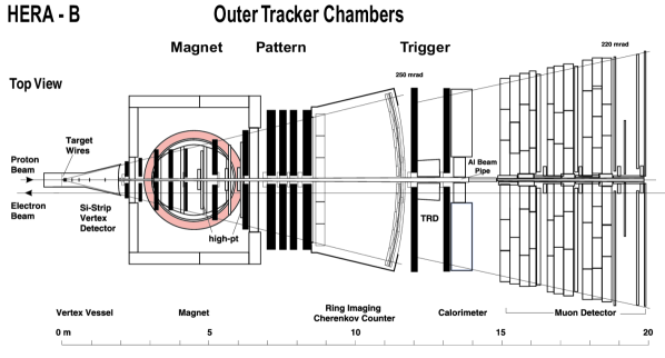
Figure 1: Schematic top view of the HERA-B experiment with the Outer Tracker chambers indicated as black bars. The $z$-axis of the coordinate system coincides with the proton beam axis.

The Outer Tracker of HERA-B serves charged particle detection from the outer acceptance limit of the experiment, defined by a 250 mrad opening angle in the bending plane of the magnet, down to a distance of 20 cm from the HERA proton beam. The OTR consists of 13 superlayers containing variable numbers of planar honeycomb drift tube layers which provide three different stereo views (wires at 0 and $\pm 80$ mrad w.r.t. vertical). Seven superlayers are located inside the magnet (labelled MC1–6,8), four between magnet and RICH (PC1–4), and two between RICH and ECAL (TC1–2). Each superlayer consists of two chambers which can be retracted from each other in $x$-direction. They are distinguished by appending $+$ or $-$ to the superlayer label, depending on which side of the proton beam tube the chamber is located. Around the proton beam the drift cell diameter is 5 mm, and the outer detector parts are equipped with 10 mm cells. In total 112 674 electronic channels provide drift time information for tracking. The detector is operated with the fast counting gas Ar/CF₄/CO₂ (65:30:5). The details of the detector and of the electronics are described in the first two papers of this series [3, 4]. Pattern recognition and track fit algorithms for the HERA-B tracking system are treated in [5].

This paper is organized as follows: The next section describes the operating conditions of the Outer Tracker. The long-term stability of several detector components, including some results on chamber aging are also presented. Its calibration and alignment, as well as the achieved spatial resolution will be discussed in Section 3. Section 4 summarizes the detector performance in terms of hit and track efficiency and momentum resolution. Finally the paper is summarized.

2 Detector Operation

2.1 Running Periods and Conditions

The Outer Tracker was routinely operated during two data taking periods of HERA-B which were separated by a long shutdown for the luminosity upgrade of HERA.

2.1.1 Run Period 2000 (July 1999 – August 2000)

This run period started with an only partially installed OTR. After completion in January 2000, the up-time of the detector was 2200 h. The first installed chambers had been operated for an additional 1100 h.

By steering the movable wire target, the proton-target interaction rate was set to values between 4 and 5 MHz most of the time, resulting in maximum channel occupancies of about 2 %. For about 20 h data were also taken at high rates of 30 and 40 MHz. Since the HERA bunch separation is only 96 ns, the high rate data contain multiple interactions per event. In total the target produced about 33000 MHz h corresponding to $1.2\cdot 10^{14}$ proton-nucleus interactions in this run period.

Despite the stable performance of HERA and the good quality of the proton beam, both resulting in very stable target rates, the OTR suffered from severe HV stability problems during this run period (see Section 2.6.1). In order to study these problems, the gas composition and the HV settings were varied. As a result, not all data were taken with the OTR operating at its nominal gas gain of $3\cdot 10^{4}$.

2.1.2 Run Period 2002 (December 2001 – February 2003)

For this run period the HERA-B physics programme focused on charm physics [6]. A re-optimization of the detector for the new physics goal led to the removal of the OTR superlayers MC2–8, with the aim to minimize the material in front of the ECAL.

Until the end of October 2002 priority was given to commissioning the upgraded HERA accelerator and only 470 h of beam time could occasionally be used by HERA-B. In the following more continuous run the OTR was operated for another 760 h.

Except for short tests, the detector was not operated at target rates beyond 5 MHz during this run period. But instabilities of HERA operation, with spikes of up to 2 GHz in the proton-target interaction rate and strong positron beam background, caused large temporary charge depositions in the Outer Tracker chambers. Occasionally currents of more than 50 times the nominal value were observed in the most exposed sectors of the detector. Usually this triggered an automatic HV switch-off procedure. Providing one chamber current as a feedback signal for beam steering to the HERA control room strongly improved the running conditions for the Outer Tracker.

Due to the improved HV stability the operational parameters of the OTR could be kept stable during this run. However, during periods of high backgrounds the detector performance suffered from distorted TDC spectra and reduced hit efficiencies. Data from such periods were excluded from physics analyses and performance studies. The useful data from this run period include $210\cdot 10^{6}$ minimum bias and $148\cdot 10^{6}$ lepton-triggered events. Most performance results in this paper have been obtained from these datasets.

2.2 Slow Control System

During data taking most of the HERA-B hardware is monitored and controlled by the Slow Control System [7]. From the Outer Tracker the ASD-8 amplifier boards, TDC crates, temperature sensors, the high voltage system, and the gas gain control are included. The system allows to remotely read and set values and to check the status of signals. The correctness of the controlled parameters is monitored by the system. If a parameter value is outside a predefined range, an alarm message is generated. The high voltage control is described in [4], the gas gain control is discussed in section 2.4. The OTR gas system [8] has its own dedicated control hardware which is also connected to the detector safety system. The system operates independently and only the gas parameters are transmitted to the general HERA-B Slow Control system.

2.2.1 ASD-8 Board Control

Low voltage distribution boards are mounted on all superlayer frames. Each board supplies up to 48 ASD-8 boards of similar sensitivity with power, thresholds, and test pulses, and monitors voltages and currents. A CAN bus connects the boards to the Slow Control System. More details can be found in [4].

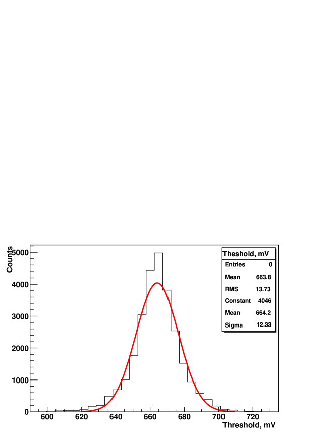
Figure 2: Threshold voltage distribution for a group of ASD-8 boards for the whole run period. A voltage of 660 mV corresponds to a charge of 2.6 fC.

Threshold stability is an important prerequisite for reliable OTR resolutions and efficiencies. The effective threshold voltage also depends on the ASD-8 supply voltages which are allowed to vary by about $\pm 10$ % ($\pm 300$ mV) before a warning is issued. Figure 2 shows the distribution of a particular threshold voltage for the whole run period. The observed r.m.s. width of 14 mV corresponds to a threshold charge uncertainty of about 0.1 fC.

2.2.2 TDC Crate Control

Each of the crates mounted on the OTR superlayer frames contains TDC boards and a daughter board of the Fast Control System (FCS) [9, 10]. The crate control monitors the voltage and temperature of the power supply and the speed of the cooling fan. It also allows to reset values of timing delays and to control the crate power.

2.3 Electronics Noise and Amplifier Thresholds

The analysis of single channel TDC spectra is the key tool to monitor the performance of every Outer Tracker channel. A normal spectrum is shown in Fig. 3 (A), while the other plots show the spectra of three classes of malfunctioning channels: Channels with asynchronous noise (B), channels with bad connections or shorts to ground (C), and channels with oscillations (D). For the data sample underlying the plots their fractions are 0.1 %, 1.8 %, and 8.8 %, respectively.

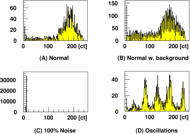
Figure 3: Typical examples of TDC spectra. A time range of 256 TDC counts corresponds to 100 ns.

The asynchronous noise of type (B) is generated by other electrical devices operating in the neighbourhood of the corresponding amplifier board. Because of different ground connections certain ASD-8 boards and channels are more affected than others. Since the timing of the electromagnetic noise is not correlated with the TDC clock, the time distribution of the noise hits is flat. Improved ground connections between the gas boxes and their ASD-8 boards almost completely eliminated this problem.

Most of the type (C) channels belonged to badly plugged ASD-8 boards. Such faulty connections were regularly fixed during access days. Just a few of them (0.014 %) were permanent due to a short to ground inside the gas box or on the feedthrough board.

Bad ground connections of ASD-8 boards to the gas box and badly shielded signal cables lead to oscillations of the amplifiers with a characteristic frequency of about 50 MHz which clearly shows up in Fig. 3 (D). This type of noise can only be suppressed by increasing the thresholds of the corresponding ASD-8 boards.

For threshold specification in the experiment a parameter $\Delta U_{thr}$ is used. It is added to the $U_{noise}$ value of each ASD-8 board. Using this parametrization one can use a common threshold parameter for all boards of one chamber which usually come from several quality classes. This makes it easy to react to changing noise conditions in the experiment. The conversion factor between threshold voltages and charges is 250 mV/fC.

In order to keep the thresholds $\Delta U_{thr}$ low and the loss of resolution and hit efficiency as small as possible, the following measures were taken: A direct connection of the analog ground of an ASD-8 board to the shielding of its output cable, a shielding of the ASD-8 board input connector to reduce the capacitive feedback from the digital output, a direct connection of the digital and analog grounds right on the ASD-8 board, and modifications of the TDC boards which reduced the feedback from their hit outputs. All these measures reduced the number of noisy channels and allowed to set lower thresholds on all chambers (see Table 1). The performance results presented in the following are based on data from the improved detector.

Table 1: Thresholds $\Delta U_{thr}$ of all OTR chambers after modification of the TDC boards. The old values are given in parentheses.

Chamber	$\Delta U_{thr}$ [mV]	Chamber	$\Delta U_{thr}$ [mV]
MC1–	100 (200)	MC1+	100 (200)
PC1–	400 (600)	PC1+	400 (600)
PC2–	500 (500)	PC2+	400 (500)
PC3–	400 (500)	PC3+	400 (500)
PC4–	400 (700)	PC4+	400 (600)
TC1–	300 (600)	TC1+	300 (500)
TC2–	300 (600)	TC2+	300 (500)

2.4 Gas Gain Control

Tests had shown that with the achievable thresholds for the frontend electronics a gas gain of about $3\cdot 10^{4}$ represents an optimum in terms of efficiency, resolution, and operational safety of the Outer Tracker chambers. Some efforts have been taken to monitor and to control this important parameter.

2.4.1 Direct Gain Measurement

A direct measurement of the gas gain has been performed at the beginning of the 2002 run period. To determine the gas gain, the current in the OTR was measured as a function of the voltage applied to the chambers. In order to reduce the uncertainty of the measurement at low voltages, where the current approaches the ionization value, the total current from about 10000 drift cells (5 mm) was measured. During the HV scan the interaction rate was kept as stable as possible.

The result is shown in Fig. 4.

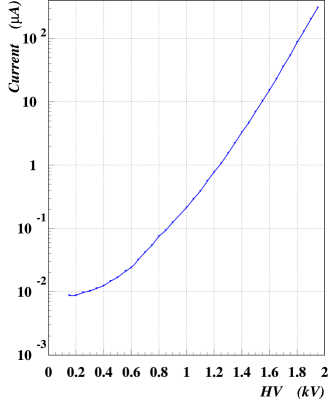
Figure 4: Sum current of $\approx 10^{4}$ drift cells (5 mm) as a function of the voltage applied to the chambers.

The gas gain $G$, defined as the ratio of the current determined at the working point and the ionization current, is found to be

$$G=\frac{I(1950\,\mathrm{V})}{I(150\,\mathrm{V})}=(3.3\pm 1.0)\cdot 10^{4}$$

This value agrees well with the results of previous gain measurements using radioactive ⁵⁵Fe sources. The large error arises from uncontrollable fluctuations of the running conditions among the points in Fig. 4 which were measured over a period of several hours.

2.4.2 Gas Gain Monitoring

The amplification in the gas mixture strongly depends on ambient conditions like atmospheric pressure and temperature, as well as on the exact composition of the counting gas. In particular the presence of oxygen has a large influence on the gas gain. For the Outer Tracker gas mixture Ar : CF₄ : CO₂ the allowed limits for variation of the fractions are ($65\pm 1$ : $30\pm 1$ : $5\pm 0.2$) %, which correspond to gain variations of about 15 %. An Outer Tracker gas monitoring system was installed to control these parameters and to act as an additional interlock if they exceed the limits [3, 8].

For gain monitoring a small chamber with 5 and 10 mm honeycomb drift cells of the OTR type is installed in parallel to the main gas input. The overlap region of both cell types is irradiated by an ⁵⁵Fe source. From the measured pulse height spectrum the positions of the pedestal ($A_{ped}$) and of the 5.9 keV gamma line ($A_{peak}$) are determined. The gain value is given in % with respect to a nominal one

$$G=\frac{A_{peak}-A_{ped}}{A_{nom}}\cdot 100\,\%.$$

$A_{nom}$ is the spectral position of the nominal gain. The used technique allows to measure gains in the range (40–150) % with an accuracy of 3 %. The measurement takes up to 15 minutes.

In order to eliminate the large but trivial influence of the atmospheric pressure on the gas gain, thus making smaller effects visible, a pressure correction is introduced. For small pressure variations this correction can be approximated by

$$\frac{\Delta G}{G}=-K\frac{\Delta p}{p}.$$

The corrected gain is obtained as

$$G_{corr}=G[1+\alpha_{p}(p-p_{nom})],$$

where $G$ and $p$ are the measured gain and pressure values, $\alpha_{p}=K/p_{nom}=0.6\,\%$ per mbar is a pressure correction factor, and $p_{nom}=1008$ mbar is the nominal atmospheric pressure in Hamburg, averaged over a year.

The gas gain monitoring system is fully integrated in the HERA-B Slow Control environment. Parameters like the atmospheric pressure, the high voltage settings, the measured and the pressure corrected gains are stored in a data base with a corresponding time stamp. The desired voltages for the two Outer Tracker cell types, which follow from the high voltage dependence of the gain, are also recorded. Figure 5 illustrates the performance of the system and shows that the largest gain variations are caused by the varying atmospheric pressure. It also shows the stability of the mixing ratio and the levels of O₂ and N₂ contamination.

Figure 5: Monitoring important gas system parameters. For clarity the pressure corrected gas gain curves for the 5 and 10 mm cells are drawn with an offset of –20 %. Day 0 corresponds to August 20, 2002.

2.4.3 Online High Voltage Steering

In order to operate the detector at an approximately constant gas gain, an automatic adjustment of the high voltage is implemented in the OTR Slow Control. The modified high voltage server retrieves the desired voltages from the data base. A modification of the high voltage is considered to be necessary if the currently applied voltages differ from the desired ones by at least 5 or 6 V for the 5 or 10 mm drift cells, respectively. Smaller differences are not significant with the given gain measurement errors. The new high voltage settings are not applied immediately but only when the Outer Tracker HV is turned on next time.

For safety reasons the steering procedure is only used to balance gains in the range ($70\ldots 140$) %, corresponding to required voltage variations of ($+1.4\ldots-2.7$) %. In addition, the desired voltage records from the data base must not be older than one hour.

2.5 Aging Investigations

Aging of the Outer Tracker drift chambers was an extensively studied R & D subject [11, 12] because of the high radiation load near the beam pipes and since there was only little experience with the fast but aggressive CF₄ gas component.

After exposure to a large radiation dose a wire chamber may exhibit an irreversible gas gain reduction. Since the chamber current at a given particle rate is proportional to the gas gain, the measured current can be used to monitor the gas gain.

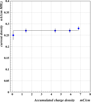
Figure 6: Current density as a function of accumulated charge. 7 mC/cm corresponds to 1000 hours of operation of HERA-B.

The current density (current per cm of wire normalized to a target rate of 1 MHz) as a function of the accumulated charge density is shown in Fig. 6. This dependence was measured in sector 4 of superlayer PC1 which is situated close to the proton and electron beam pipes where the density of the accumulated charge is maximal (see [3] for sector definitions). As follows from Fig. 6, there is no visible decrease of the current (and therefore of the gas gain) within an accuracy of 5 % for an accumulated charge density up to about 7 mC/cm. This charge density corresponds to the operation of the HERA-B detector for more than 1000 hours during the 2002 run period. During its entire operation time the Outer Tracker accumulated an average charge density of 24 mC/cm on the anode wires in the hottest regions.

Due to the much shorter than scheduled run of HERA-B and to mostly running at target rates of 5 MHz or even less, the accumulated charge density does not seriously probe the OTR design criterion of being able to collect up to 1.5 C/cm during five years of running at 40 MHz.

After the run end an anode wire which was located near the proton beam pipe was taken out of the MC8 chamber and investigated using an electron microscope. The wire surface is mostly clean, some very isolated depositions contain oxygen, silicon, chlorine, potassium, and sodium. There is no hint for wire etching which had been observed as a function of gas humidity in earlier studies [12].

2.6 Detector Stability

2.6.1 High Voltage Stability

The most disturbing OTR problem during the 2000 run was the continued loss of high voltage groups. From the very beginning of OTR operation in July 1999 it was observed that HV groups occasionally failed. The average long term rate of these failures was one HV group per 5 hours up-time of the Outer Tracker, but there were strong fluctuations. Since a HV group supplies 16 wires, the failure of a single wire causes a channel loss which is a factor 16 higher.

Mechanical Instabilities:

The failure rate was especially high in TC2–, the first assembled and installed large chamber. Here it was suspected that this was caused by mechanical instabilities of the modules, none of which was reinforced yet with carbon fibre rods. Most modules in all later installed chambers had this reinforcement [3]. In a complete overhaul of TC2– in December 1999 the chamber was disassembled, all modules were reinforced and subjected to a more rigorous HV test than before. With reference to a flat table, the module was bent with a sagitta of 8 mm, a condition similar to what was observed on modules installed in TC2– during the first assembly. All wires which then showed shorts or excessive dark currents were disabled. Compared to the original test procedure which only checked perfectly flat modules, the number of eliminated wires roughly doubled, raising the fraction from 0.6 to 1.1 %. During the 8 months of running time after this repair only 16 of 606 HV groups in TC2– showed problems, compared to 115 groups during the 5 months before the repair.

Shorts on HV Boards:

By the end of the 2000 run there were 499 defect HV groups (out of 7219 in total) in the whole Outer Tracker, not counting the TC2– problems in 1999. The inspection of damaged modules revealed a somewhat unexpected major source of the problems: In more than 90 % of the cases the “short” was caused by a burnt-in carbon trace of varying resistance across either of two capacitors on the bottom side of the HV distribution board. In no case any of the 15 top side capacitors caused the problem. This systematic difference had to do with the differing mounting techniques used for top and bottom side components in the SMD soldering process [4]. Less than 10 % of the faulty HV groups had genuine drift cell shorts which were caused by mechanical module damage during installation, wire instabilities in modules without reinforcement, and instantaneous wire breaking under extremely high radiation load (rate spikes related to beam loss).

During the 10 months of the shutdown all chambers were disassembled and the modules were subjected to the same repair steps as described above for TC2–. The most time-consuming step in this procedure was the manual exchange of 12 000 SMD filter capacitors on the HV distribution boards.

Other losses of HV groups:

Repaired and reinstalled chambers were kept at nominal high voltage for at least three days, but the first repaired chambers were trained for as long as 82 days. During this phase 55 HV groups were lost, mostly due to installation damage. During the first phases of the 2002 run, when the OTR was only occasionally operated, 33 HV groups were damaged. This was mostly related to special events like a HV scan up to twice the nominal gas gain, or frequent chamber movement for maintenance. For certain types of modules the internal stability was not good enough to withstand the vibrations during chamber handling. During the final 760 h of regular OTR operation in 2002/2003 only 10 HV groups developed shorts, and more than half of these occurred during extreme background conditions at the accelerator.

2.6.2 Component Stability

From 1999 to 2003 the complete OTR was operated for more than 3400 h, some chambers saw up to 1100 h additional beam time (see Sec. 2.1). This makes quantitative statements about the long term stability of various system components possible.

Detector Modules:

The OTR was assembled from about 150 different types of detector modules [3]. After reinforcement with carbon fibre rods the vast majority of these showed sufficient mechanical rigidity, resulting in good electrostatical stability during operation. In retrospect it must be said, however, that the modules with 5 mm cells were designed too close to the stability limit, with free wire lengths of 59 and 68 cm between support strips [3] in the PC and TC chambers, respectively. Most HV instabilities were observed in this region of the detector and 80 of 978 modules were rebuilt when repairing the detector during the HERA shutdown.

Gas System:

The most problematic components of the gas system were the metal bellow circulation pumps [8]. At times 5 of the 15 pumps were out of order thus reducing the gas flow rate to only 70 % of the nominal value. In all cases the problems were caused by leaking bellows. These leaks were most probably induced by solid contaminants inside the closed gas loop. Occasional problems in the gas mixing system and in the pressure regulation loops were mostly solved by recalibrating the mass flow controllers. Only once such a problem was caused by the complete breakdown of the steering unit.

3 Detector Calibration

In order to obtain the spatial coordinates of the track hits from the measured TDC values, several sets of calibration and alignment constants are necessary:

1. Bad channels are identified and recorded in channel masks which are used differently in online and offline tracking procedures.

2. The TDC spectra from all detector channels are corrected for individual time shifts $t_{0}$. These constants are generated by the $t_{0}$-calibration.

3. The translation of TDC counts to drift distances is done by means of a drift time to distance relation $r(t)$. The resolution function $\sigma(t)$ provides the errors of the measured distances. For each cell type both functions are generated by the $rt$-calibration.

4. Finally, the measured coordinates must be corrected by alignment constants which account for deviations of detector elements from their nominal geometry. The internal alignment determines Outer Tracker distortions, the global alignment the OTR displacement in HERA-B.

A set of calibration constants remains valid as long as the corresponding detector properties do not change. Failing hardware, threshold manipulation, and chamber movements during the run periods call for several instances of all sets. They are all stored in the HERA-B Calibration-and-Alignment (CnA) Database [13].

3.1 Masking of Bad Channels

Bad Outer Tracker channels must be excluded from being used in pattern recognition and track fit because they can disturb the procedures. They are best identified in occupancy maps of the OTR chambers. An occupancy map is a normalized hit map. For each wire it gives the number of recorded hits divided by the number of analyzed events (channel occupancy). Bad channels are found by comparing for every wire the measured channel occupancy with the occupancy predicted by a Monte Carlo (MC) simulation. Depending on whether their occupancies are much higher or much lower than expected, bad channels are called either noisy or dead.

Measured occupancies strongly depend on the interaction rate and on the trigger configuration. In order to compare arbitrary experimental data with a standard MC sample, measured channel occupancies are scaled by the ratio of the total numbers of hits in simulation and data. When this scaling is applied, there remains only a small influence of the trigger configuration, as was assessed by analyzing runs using different triggers. The influence of the material and the position of the target is also small.

In the MC simulation 300 000 minimum bias events were generated and processed through a detailed GEANT detector simulation [14]. This is done only once per run period, assuming a stable geometry of HERA-B. The calculated wire occupancies, the number of events, and the total number of hits are stored.

For each set of experimental data 50 000 events are analyzed. The measured occupancies are properly scaled and compared to the MC reference. Noisy and dead wires are identified using the cuts described below. The generated channel mask is stored in the calibration database.

An example for the distribution of measured versus MC predicted occupancies for each wire is shown in Fig. 7.

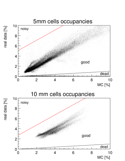
Figure 7: Distributions of measured vs. MC predicted occupancies for 5 and 10 mm cells. Most noisy wires have occupancies close to 100 % and are out of range in this plot.

Wires with measured occupancies $\Omega_{meas}$ smaller than 10 % of the MC predicted value $\Omega_{MC}$ are marked as dead. This cut is indicated by the lower lines in Fig. 7. The optimal cuts to define noisy wires are

$$\Omega_{cut} = \Omega_{MC}+\langle\Omega_{meas}\rangle\cdot 1.5\quad\textrm{for 5\,mm cells,}$$

$$\Omega_{cut} = \Omega_{MC}+\langle\Omega_{meas}\rangle\cdot 0.8\quad\textrm{for 10\,mm cells.}$$

They are indicated by the upper lines in Fig. 7. These definitions accept a relatively large fraction of noise hits on wires for which the simulation predicts small occupancies. This helps to maximize the number of usable channels and is tolerated by the track reconstruction algorithms as long as the absolute number of hits remains low. More details and comparisons with other masking methods can be found in [15].

Table 2 shows for a typical run the fractions of good, noisy, and dead wires in all chambers of the Outer Tracker.

Table 2: Fractions of good, noisy, and dead wires in all chambers of the Outer Tracker for a typical run.

Superlayer	good [%]		noisy [%]		dead [%]
side	$+x$	$-x$	$+x$	$-x$	$+x$	$-x$
MC1	93.1	94.5	0.1	0.1	6.8	5.4
PC1	93.1	94.7	0.4	0.5	6.5	4.8
PC2	94.2	94.1	1.2	0.6	4.6	5.2
PC3	94.1	94.8	3.0	1.1	3.0	4.2
PC4	91.7	95.9	0.8	0.3	7.5	3.8
TC1	90.4	93.2	0.5	0.3	9.2	6.5
TC2	91.2	90.8	0.7	3.0	8.1	6.2

It should be noted that masked cells are treated differently in the different parts of the trigger chain and in the track reconstruction. In order to prevent an unacceptable loss of trigger efficiency, the First Level Trigger considers noisy wires as good and dead cells as always having a hit, even though this leads to an increased number of trigger messages. Contrary to this, masked cells are excluded from the Second Level Trigger and from the online and offline track reconstruction.

3.2 TDC Spectrum Shifts

The hardware calibration of the TDCs maps a time interval of 100 ns linearly to 256 TDC counts [4]. Linearity and stability of the conversion factor are so good that it adds negligibly to the final uncertainty of the time measurement. The origin of the time scale is not so well defined, the absolute timing depends on the channel. In order to be able to use a common drift time scale throughout the Outer Tracker, the TDC spectra of all detector channels are time aligned using individual time shifts $t_{0}$. These calibration constants absorb systematic effects arising e.g. from differences in cell position or signal propagation time.

The $t_{0}$ calibration procedure evaluates the truncated means of the TDC spectra [16]. The truncation limits $t_{min}$ and $t_{max}$, given in Table 3, are chosen to accept 95 % of all hits. The difference of the truncated mean and the reference value $t_{ref}$ yields the time offset $t_{0}$ for each channel. The $t_{ref}$ values shown in Table 3 were chosen at the beginning of the run to minimize the average $t_{0}$.

Table 3: Limits for the truncation of the TDC spectra and reference values for the $t_{0}$ calculation (all in TDC counts).

Cell Size	$t_{min}$	$t_{max}$	$t_{ref}$
5 mm	130	230	180
10 mm	50	250	150

Due to the truncation this extremely simple procedure must be iterated, but already after the third iteration the $t_{0}$ values are stable within 0.5 ns, the time measurement bin of the TDC.

The quality of this $t_{0}$ calibration procedure can be assessed by comparing summed TDC spectra before and after application of the $t_{0}$ corrections. As is shown in Fig. 8 for both types of drift cells, the corrected spectra have a higher peak and a steeper rising edge than the uncorrected ones, just as one would expect from improving the overlap of the single wire spectra. On the other hand, the effect is small which shows that the rough $t_{0}$ calibration done by setting delays on the Fast Control System (FCS) daughter boards in the TDC crates is already quite good (see section 2.2.2).

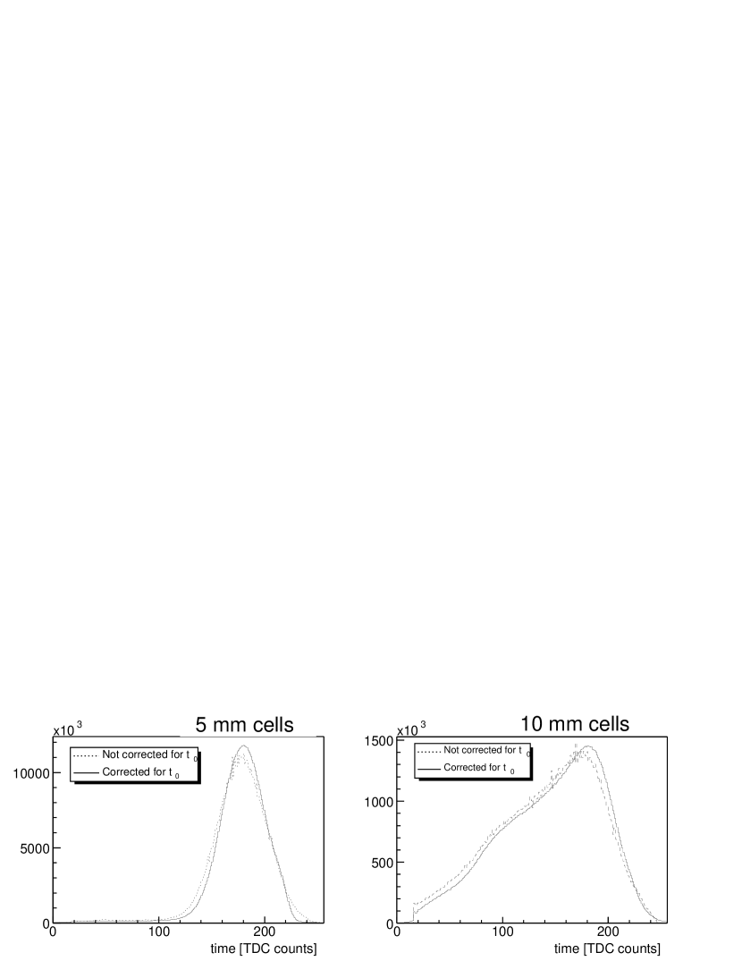
Figure 8: Summed TDC spectra of all cells (dotted line without, solid line with $t_{0}$ correction). Since the TDCs operate in “Common Stop” mode, the time scale is inverted, i.e. large TDC counts correspond to short drift times and vice versa.

The $t_{0}$ constants were determined for each run with more than 300 000 events. As an illustration of the long term stability of the $t_{0}$ calibration, the differences of the values obtained for three runs in a period of six weeks are shown in Fig. 9. The shift of the left spectrum by $-2.25$ TDC counts is a consequence of changed operational parameters. The small structures at $+10$ and $-20$ TDC counts are attributed to instabilities of the FCS delays for single crates. These were cured by resetting the affected TDC crates.

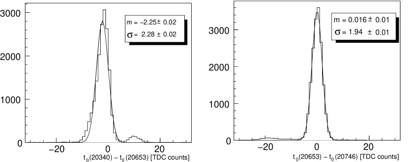
Figure 9: Long term stability of the $t_{0}$ calibration: Differences of $t_{0}$ values determined for the runs 20340, 20653, and 20746, taken during a time period of six weeks.

3.3 Drift Time to Distance Calibration

The drift time to distance relation $r(t)$, or $rt$-relation for short, transforms a measured drift time $t$ into a distance $r$ from the hit wire. The resolution function $\sigma(t)$ provides the errors of the measured distances $r(t)$. Both functions are needed when preparing hits for pattern recognition and track fit. They are determined in a common $rt$-calibration procedure. A detailed description of the HERA-B Outer Tracker $rt$-calibration is given in [16]. Here only the main features of the procedure are summarized and some results on the average hit resolution are presented.

3.3.1 Calibration Procedure

Using the drift distances $r(t_{i})$ of all hits $i$ found by the pattern recognition for a certain track, the track fit yields five parameters which fully describe the track [5]. Using these parameters, one can calculate distances of closest approach $d_{i}$ of the track to the anode wires of all used drift cells. While $r(t_{i})$ is an unsigned quantity, namely the radius of a cylinder around the wire which the particle track must be tangent to, the calculated distance $d_{i}$ has a sign that tells on which side the track has passed the wire. For a quantitative comparison of measured and predicted distances the left-right ambiguity of $r(t_{i})$ is solved in the track fit by applying a sign parameter $\epsilon_{i}$ such that the square of the residual

$$\Delta_{i}=\epsilon_{i}\,r(t_{i})-d_{i}$$ (1)

becomes minimal. After convergence of the track fit one has $\epsilon_{i}=\mathrm{sign}(d_{i})$ for every hit.

The predicted distance $d_{i}$ depends on all hits participating in the track fit and therefore is a good estimator for the “true” distance of the track from the wire. Hence, if only an approximate $r(t)$ is used for the hit preparation, an improved $rt$-relation can be obtained from the correlation of predicted distances $d$ and measured drift times $t$. Figure 10 shows examples of this two-dimensional distribution for 5 and 10 mm drift cells in the PC superlayers.

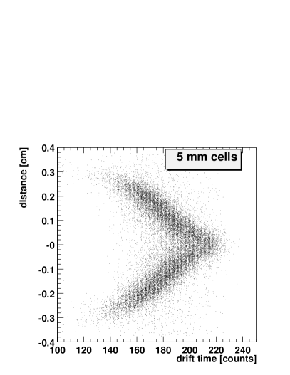
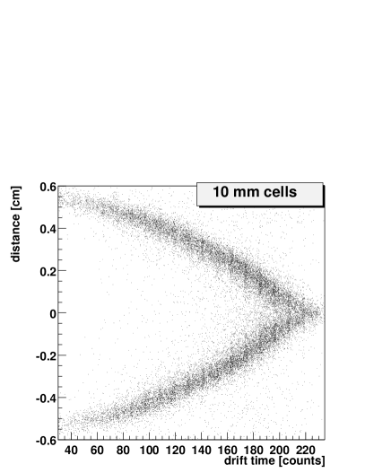
Figure 10: Signed reconstructed distance versus measured drift time for 5 and 10 mm cells in the PC chambers. One TDC count is 100/256 ns. Because of operation in “Common Stop” mode high TDC counts correspond to short drift distances.

In each drift time bin the average value $\langle|d|\rangle$ of the unsigned predicted distances is calculated. The resulting data points are smoothed in a least squares fit using third order B-spline polynomials. These eventually yield the values of the new $rt$-relation. Figure 11 illustrates such an $rt$-calibration step. From the plots one can also deduce quite high drift velocities of about 115 and 90 $\mu$m/ns in the centers of the 5 and 10 mm drift cells, respectively.

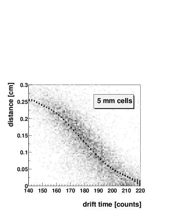
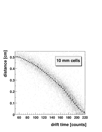
Figure 11: Interpolated points of the $r(t)$ functions for 5 and 10 mm cells. The input distributions $|d|(t)$ are shown as well.

The value of the resolution function $\sigma(t)$ in a given drift time bin follows from the RMS width of the distribution of residuals (1) in that time bin. Also here the measured points are smoothed using a B-spline fit. Since all hits which populate the residual distributions are also used in the track fit, an individual scaling factor must be applied to each residual, in order to compensate for the introduced bias [16]. Figure 12 shows distributions of scaled residuals as a function of the measured drift times for both types of drift cells. For each time bin the RMS width of the residual distribution, i.e. the value of the new resolution function is shown as a point.

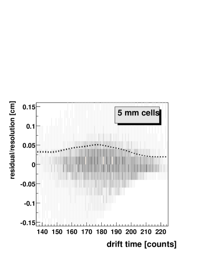
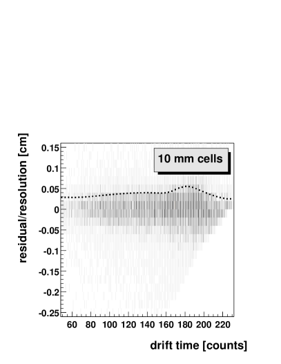
Figure 12: Resolution functions $\sigma(t)$ for 5 and 10 mm drift cells (dotted lines). The input distributions $\Delta(t)$ are shown as well.

The described steps of obtaining new functions $r(t)$ and $\sigma(t)$ define an iterative procedure. Typically five iterations are sufficient to converge to the required precision. For track reconstruction in the first iteration $r(t)$ is obtained by integrating the drift time spectrum and the resolution is assumed to be constant at 1 mm.

The $rt$-relation discussed here is a tabulated function which is used for the transformation of TDC counts to distances. It is determined using tracks going through the whole detector and thus is influenced by global effects like variations between drift cells, misalignment, variations in interaction time, and by properties of the track reconstruction procedure itself. In certain details this phenomenological function may be quite different from the physical $rt$-relation of a drift cell which is defined by the operating parameters of the cell (e.g. electric and magnetic field, drift gas mixture, pressure, temperature) and modified by properties of the attached readout electronics (e.g. impedance, threshold, pulse shaping).

The same arguments apply for the resolution function. The improvement of $\sigma(t)$ towards the sense wire (large TDC counts in Fig. 12) which contradicts the expectation from drift chamber physics, results from the described method of resolving the left-right ambiguity. This method suppresses negative residuals $\Delta(t)<-r(t)$ and leads to asymmetric and artificially narrow distributions close to the wire. Here $\sigma(t)$ still yields the correct hit weight for the track fit, but it is no longer identical to the physical drift chamber resolution.

The technical nature of both functions is emphasized by using a hardware defined time scale of TDC counts instead of proper drift times in nanoseconds.

3.3.2 Performance on Data

Figure 13 shows the distributions of scaled residuals for 5 and 10 mm cells in the PC chambers of the Outer Tracker. In both types of cells an average resolution of about 370 $\mu$m is obtained. This includes a substantial contribution from multiple scattering because the chambers in the PC region represent an average thickness of 0.15 radiation lengths while for statistics reasons the calibration procedure uses a track momentum cut of only 5 GeV/c.

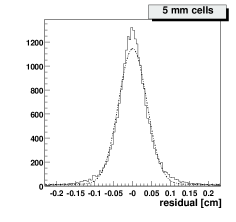
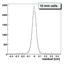
Figure 13: Distributions of scaled residuals for 5 and 10 mm cells in the PC chambers of the Outer Tracker. The dashed lines represent Gaussian fits. The average resolution is about 370 $\mu$m in both cell types.

In order to investigate this further, the average resolution of the 5 mm cells is determined as a function of track momentum. For this purpose high quality tracks are selected which have at least 20 hits in the PC chambers and which are also observed in the silicon vertex detector and in the TC chambers. In each of the chambers PC2 and PC3 one layer is excluded from pattern recognition and track fit. In these layers distributions of unbiased residuals are accumulated in bins of track momentum. The result is shown in Fig. 14. The measured data are compatible with a chamber resolution of 300 $\mu$m and multiple scattering contributions of 80 and 310 $\mu$m at $p=20$ and 5 GeV/c, respectively.

Figure 14: R.m.s. width of the residual distribution for 5 mm drift cells as a function of track momentum.

A chamber resolution of 300 $\mu$m falls outside the range 150–250 $\mu$m, the design target in the proposal [1], which was verified in several series of test measurements [17]. This is mostly due to the elevated noise level in the full detector compared to limited test setups (see Sec. 2.3). The required higher settings for the discriminator thresholds worsen the resolution. For a large system with more than 100 000 channels also the threshold granularity becomes important [4] because it defines how closely the detector can be adapted to spatially varying noise conditions. Finally, a full tracking system of independent chambers also suffers more from alignment and calibration uncertainties both of which adversely affect the spatial resolution.

3.4 Alignment

There are two independent alignment tasks: The internal alignment deals with the relative positions of the individual OTR modules, while the global alignment determines the spatial position of the OTR with respect to the other components of HERA-B.

3.4.1 Internal Alignment Considerations

An internal alignment procedure for the HERA-B Outer Tracker must meet certain demands:

• It must use tracks reconstructed in the OTR itself because there are no external tracks of sufficient precision available.

• It must be able to work with hadronic tracks that are found in typical HERA-B events with only a moderate momentum cut being applied (typically 5 GeV/c). Such a track sample can be collected within a few hours and covers the full acceptance of the detector. This is adequate for the sometimes quite short intervals of stable detector geometry.

• It must be robust against a possible bias introduced by the track reconstruction procedure. The problem with the above track sample is the large spatial track density per event and hence the proper assignment of hits to tracks. If no measures are taken any track reconstruction algorithm will pick up the nearest hits and will prefer left-right signs for the drift distances that minimize the residual squares, thus creating a background in the residual distribution that peaks at zero.

In the following section an iterative algorithm is described which meets the above demands. Possible improvements by other algorithms have been investigated [18] but have not become relevant for the HERA-B data analysis.

3.4.2 Iterative Method of Internal Alignment

The HERA-B geometry is described by a data structure called GEDE (GEometry of DEtector). In the following this name will be used to denote the smallest OTR units to be aligned, the sensitive sectors of OTR modules [3]. There are in total 1380 GEDE units within the PC/TC area. GEDE units belonging to the same module are mechanically coupled but for simplicity such constraints are neglected. Each GEDE unit $k$ is treated as a rigid body and two alignment constants are considered: $a^{u}_{k},a^{z}_{k}$, where $u$ means the direction orthogonal to the wire, $z$ is the direction along the beam. The stereo angle $\alpha$ is treated as a constant.

If the alignment is based on internal tracks, all GEDE parameters become correlated. Instead of a proper treatment of the large correlated system we simplify the problem and consider each GEDE as an independent unit. The algorithm is then based on the residual distributions for each individual GEDE plane. To avoid the above mentioned uncertainties of the track-to-hits association, for each track the residuals are calculated for all hits in the traversed GEDE. Also for the left-right ambiguity of the drift distance measurement no decision is made at this point, but both signs are accepted. This is done by creating two residual histograms $h_{+}$ and $h_{-}$ per GEDE plane, which are filled using always the positively or negatively signed drift distance, respectively. The left hand plots in Fig. 15 show the characteristic shapes of these histograms:

Figure 15: Combining two residual histograms using always positive or negative drift distance signs.

There is a flat background from calculating residuals using hits in wrong cells, a shoulder from calculating residuals using hits from the right cell but with wrongly signed drift distances, and a peak resulting from properly calculated residuals. The peak occurs at the same position in both histograms.

In order to improve the computational robustness of automatic peak fitting, after processing all events the histograms are combined binwise: For each bin $i$ we set $h^{i}=\min(h^{i}_{+},h^{i}_{-})$. This symmetric histogram (see Fig. 15) does neither depend on the hit-to-track association nor on the left-right ambiguity resolution, and even for large offsets a clear peak can be observed. The fitted peak position is used as an alignment correction $a^{u}_{k}$ and the track reconstruction is repeated iteratively as long as there is an improvement. Beyond a certain alignment accuracy the residual width is dominated by multiple scattering. Therefore the standard deviation of the residual mean distribution is used as a control parameter. Typically after 20 iterations this quantity is less than 50 $\mu$m and does not improve any further.

3.4.3 External Degrees of Freedom and Layer $z$ Corrections

The described algorithm does not fix the alignment constants uniquely. In general any global transformation that maps straight tracks into straight tracks will give a valid set of alignment constants:

$$\tilde{a}^{u}_{k}=a^{u}_{k}+[T^{x}+S^{xz}z_{k}]\cos\alpha_{k}-[T^{y}+S^{yz}z_{k}]\sin\alpha_{k}$$

Here $T^{x}$ and $T^{y}$ are global offsets in $x$ and $y$, $S^{xz}$ and $S^{yz}$ are shearings, i.e. offsets that depend linearly on $z$. The stereo angle for a given GEDE is denoted by ${\alpha_{k}}$. For each iterative step we choose the global offsets and shearings such that they minimize the summed squares of the alignment constants $\sum_{k}(\tilde{a}^{u}_{k})^{2}$.

Finally from the alignment constants $\tilde{a}^{u}_{k_{l}}$ belonging to layer $l$ the average $z$ shift $a^{z}_{l}$ for this layer can be estimated by minimizing $\sum_{k_{l}}(\langle\tan\theta_{k_{l}}\rangle a^{z}_{l}+\tilde{a}^{u}_{k_{l}})^{2}$. Here $\langle\tan\theta_{k_{l}}\rangle$ is the average track slope for the GEDE plane $k_{l}$. The error of $a^{z}_{l}$ is about a factor $1/\langle\tan\theta_{l}\rangle$ larger than the average error of the $\tilde{a}^{u}_{k_{l}}$, $\langle\tan\theta_{l}\rangle$ being the average track slope in layer $l$. For the PC chambers one has $\langle\tan\theta_{l}\rangle\approx 0.14$, leading to $z$ shift precisions of about 350 $\mu$m.

3.4.4 Global Alignment

The above procedure does not define the position of the OTR within the HERA-B coordinate system. To define this global alignment, external tracks are necessary. Here the problem appears that the tracking through the HERA-B magnetic field depends on the track momentum and the measurement of the track momentum depends on the global alignment. To avoid this circular argument, special sets of alignment data have been taken with the magnet switched off. This allows for a straightforward determination of the relative position of the OTR.

The data samples used for the global OTR alignment were large enough to obtain statistical errors of the alignment parameters which were small compared to the coordinate resolution. In practice the systematic uncertainties of the parameters were much bigger than the statistical errors. Their effect on the momentum resolution will be discussed in Section 4.4.

4 Detector Performance

4.1 Cell Hit Efficiency

The cell hit efficiency is the probability to register a signal in an Outer Tracker drift cell after the passage of a charged particle. This is one of the essential quantities which characterises the detector performance and which has a strong impact on the track and trigger efficiencies. A charged particle passing a stereo layer should hit at least one cell in each single layer and two cells in each double layer. Counting the layers, the expected number of hits would be 30 in the PC and 12 in the TC chambers. Due to the overlap of cells and modules, the real number of hits can be larger.

In order to study the cell hit efficiency, high statistics track samples have been selected using the following requirements:

• Events must be reasonably populated, with a total number of hits $900<N_{hits}<8000$ in the OTR chambers.

• Tracks must traverse the whole detector, with segments in the Vertex Detector (VDS) and in the PC and TC Outer Tracker superlayers.

• Tracks must have enough hits per segment, with $N^{VDS}>6$, $N^{TC}+N^{PC}>20$, and $N^{TC}>6$.

• Tracks must have a momentum $p>5$ GeV/c to keep multiple scattering small.

• Track segments must point to the target, with a vertical coordinate of the extrapolated segment at the target position $|y_{target}|<25$ cm.

A segment is approximated by a straight line connecting the first and last point of the segment. This line is used to predict the hit positions in all traversed drift cells. For each cell two histograms are filled: $N^{found}(x)$ and $N^{expect}(x)$, i.e. the found and expected numbers of hits, respectively, at the distance $x$ from the segment to the wire. The hit efficiency is calculated as

$$\epsilon_{hit}(x)=\frac{N^{found}(x)}{N^{expect}(x)}\,$$

Fig. 16 shows an example of such a cell efficiency profile.

Figure 16: Example of an efficiency profile for a 5 mm drift cell.

To extract the single cell efficiency, the measured efficiency profile is fitted by a function with six free parameters. The most important ones are the maximum of the efficiency profile, the smearing of its edges due to cell geometry and track parameter errors, the background level which describes the average occupancy, and the shift of the cell profile due to misalignment. The method and the fitting procedure are described more detailed in [19, 20].

The resulting average cell efficiency per chamber, i.e. the mean value of the cell efficiency profile maxima, for 5 and 10 mm cells is summarized in Table 4 for a typical run.

Table 4: Average cell efficiencies (in %) for 5 and 10 mm cells in all PC and TC chambers for a standard run.

Superlayer	$-x$		$+x$
	5 mm	10 mm	5 mm	10 mm
PC1	95.8	97.5	94.9	98.2
PC2	95.0	97.2	92.3	98.2
PC3	96.2	98.2	96.3	98.5
PC4	95.0	96.8	94.2	94.7
TC1	95.6	97.7	94.4	96.9
TC2	92.2	95.4	89.8	93.2

The average hit efficiency is about 94 % for 5 mm cells and 97 % for 10 mm cells. This is consistent with the expectation of a higher efficiency for a larger drift cell at the same gas gain. The observed lower efficiencies of superlayer TC2 are not completely understood.

Hits which are used twofold, first defining the track and then estimating the efficiency, can bias the hit efficiency result. This was studied by exclusion of a stereo layer from tracking and showed the bias to be less than 1 %.

The First Level Trigger (FLT) of HERA-B utilizes three stereo double layers in each of the chambers PC1, PC4, TC1, and TC2. In order for a track to be triggered hit signals must be found in all 12 double layers, with each hit being the logical OR of two lined-up drift cells. A single cell hit efficiency $\epsilon_{hit}$ then limits the trigger efficiency to

$$\epsilon_{trig,max}=[1-(1-\epsilon_{hit})^{2}]^{12}.$$

For $\epsilon_{hit}=94\,(97)\,\%$ this yields $\epsilon_{trig,max}=95.8\,(98.9)\,\%$, which can be compared to the measured efficiency for FLT tracking in the OTR layers, averaged over the 2002 run, of approximately 60 %. The additional inefficiencies come from limitations of the FLT tracking algorithm and data transmission problems in the optical links connecting the OTR front-end electronics to the FLT processor network.

4.2 Tracking Efficiency

The tracking efficiency is a basic quantity for most of the physics analyses. The evaluation method developed for the OTR of HERA-B [21] uses a sample of reference tracks which are reconstructed without using the OTR. A reference track consists of a track segment in the VDS together with an associated RICH ring or ECAL cluster. In order to keep the contamination by unphysical tracks (e.g. detector or reconstruction artefacts) in the reference sample low, each reference track must be consistent with originating from a $K^{0}_{S}\to\pi^{+}\pi^{-}$ decay. For all pairwise combinations of reference tracks and partner tracks with at least a VDS and an OTR segment the invariant mass is calculated, and the fitted number of $K^{0}_{S}$ particles in the mass spectrum is defined to be the number of reference tracks $N^{RICH}_{ref}$.

Then in the vicinity of each reference track an OTR segment matching with the same VDS segment is searched. If one is found, the track momentum is recalculated, and another invariant mass spectrum is generated as described above. A fit to this spectrum yields the number of reference tracks confirmed by the OTR, $N^{OTR}_{ref}$.

Figure 17: Determination of $N^{RICH}_{ref}$ and $N^{OTR}_{ref}$. (a) All particle candidates with VDS-RICH reference tracks which survive the selection cuts. (b) Particle candidates with OTR segments matching the reference tracks. The momentum of the reference track is replaced by the momentum of the corresponding VDS-OTR track.

Figure 17 shows an example of corresponding mass spectra and fits. The surprising fact that $N^{OTR}_{ref}>N^{RICH}_{ref}$ is due to the higher probability for wrong matches in the VDS-RICH track sample. There are $K^{0}_{S}$ candidates which only show up when the better quality VDS-OTR track is used in the invariant mass calculation.

Figure 18: Correlation between the invariant masses of reference particles computed with the momenta from VDS-RICH and VDS-OTR tracks, respectively.

This effect can be observed in Fig. 18 where side band events in the VDS-RICH sample have the proper invariant mass for the corresponding VDS-OTR tracks. The effect of such tracks must be excluded from the efficiency calculation.

The determination of the number of reference particles $N^{OTR}_{side}$ which contribute to the $K^{0}_{S}$ peak of the $m_{\pi^{+}\pi^{-}}^{OTR}$ spectrum, but are in the side bands of the $m_{\pi^{+}\pi^{-}}^{RICH}$ spectrum, is similar to that of $N^{OTR}_{ref}$ described above. The only difference is that all VDS-RICH reference particle candidates with masses in the range $m_{K^{0}_{S}}^{RICH}\pm 3\sigma_{K^{0}_{S}}^{RICH}$ (see Fig. 17a) are excluded. A scaling factor $f$ must be introduced to extrapolate the number $N^{OTR}_{side}$, which is determined in the side bands, to the full mass range. Then the tracking efficiency can be calculated as

$$\epsilon=\frac{N^{OTR}_{ref}-f\cdot N^{OTR}_{side}}{N^{RICH}_{ref}}.$$

The efficiencies evaluated for the OTR in the 2002 running period are about 95–97 %, as shown in Table 5.

Table 5: An example of tracking efficiency results for data from the 2002 running period.

Mode	$N^{Mode}_{ref}$	$N^{OTR}_{ref}$	$N^{OTR}_{side}$	$f$	$\epsilon$
RICH	$7031\pm 94$	$8230\pm 93$	$1095\pm 35$	$1.34\pm 0.02$	$0.965\pm 0.020$
ECAL	$4588\pm 78$	$5417\pm 77$	$787\pm 30$	$1.35\pm 0.02$	$0.954\pm 0.026$

An important point to be noticed is that the efficiency estimation with this method includes both the OTR tracking efficiency and the matching efficiency between VDS and OTR segments. This is no disadvantage because the physics analyses require the total efficiency anyway. In Sec. 4.3 the VDS-OTR matching efficiency is estimated to be 98 % for pion tracks, which means that the proper OTR tracking efficiency is even about 2 % higher than the numbers displayed in Table 5.

4.3 Efficiency of Track Matching

Track segments are reconstructed independently in the VDS and in the OTR PC chambers. The vector of track segment parameters at a reference $z$ coordinate is

$$\mathbf{V}^{\rm T}=(x,\;y,\;t_{x},\;t_{y},\;q),$$

where $x$ and $y$ are the transverse coordinates, $t_{x}=p_{x}/p_{z}$ and $t_{y}=p_{y}/p_{z}$ are the track slopes, and $q=Q/\left|\vec{p}\right|$ is the ratio of the charge $Q$ and the particle momentum $\left|\vec{p}\right|$.

Matching VDS and PC track segments goes through the following steps:

1. Initially the vectors of segment parameters in the VDS ($\mathbf{V}^{i}_{VDS}$) and in the PC region ($\mathbf{V}^{j}_{PC}$) together with their covariance matrices are only partially known, because the component $q$ is not yet defined.

2. A function performing a Kalman filter fit finds all pairs $\mathbf{V}^{i}_{VDS}$ and $\mathbf{V}^{j}_{PC}$ which fit to each other. The $\chi^{2}$ of the fit is a measure of the matching quality.

3. For each matched pair the fit yields a track parameter $q$, which is common to both segments.

The matching $\chi^{2}$ in step 2 does not follow a $\chi^{2}$ distribution because the track parameter differences from the Kalman filter step are not Gaussian distributed. The reasons are Molière scattering of particles, hit corruption by background particles, and failures of pattern recognition due to erroneous hit-segment assignment or wrong left-right assignment of drift distances in the OTR.

In order to find a reasonable cut value for the matching $\chi^{2}$, the reconstruction efficiencies of $K^{0}_{S}\to\pi^{+}\pi^{-}$ and $J/\psi\to\mu^{+}\mu^{-}$ decays were investigated for different cuts on the matching $\chi^{2}$ [22]. From the invariant mass spectra of $\pi^{+}\pi^{-}$ and $\mu^{+}\mu^{-}$ combinations the number of events in the corresponding peaks and the combinatorial background underneath were evaluated. The results are shown in Fig. 19.

Figure 19: The number of (a) $K^{0}_{S}\to\pi^{+}\pi^{-}$ decays and (b) $J/\psi\to\mu^{+}\mu^{-}$ decays together with the combinatorial backgrounds underneath the signal peaks as functions of the cut on the matching $\chi^{2}$.

For very soft cuts on the matching $\chi^{2}$ all proper pairs of segments are matched and the number of events in the peak reaches a plateau, but also the probability to match wrong pairs becomes large and the background increases. Cutting the matching $\chi^{2}$ at 200, the default value for data processing, the number of reconstructed $K^{0}_{S}$ decreases by only $(3.3\pm 0.1)\,\%$ from the plateau value (see Fig. 19a). This results in a matching efficiency of about 98 % for a single pion track.

The muons from the $J/\psi$ decays are more energetic than the pions and also have better chances to be reconstructed and matched because they have already been selected by the trigger. As can be seen in Fig. 19b, the number of reconstructed $J/\psi$ particles already reaches a plateau for matching $\chi^{2}$ cuts much smaller than 200. Hence with the default cut the matching efficiency for energetic muons is close to 100 %.

4.4 Momentum Resolution

The momentum resolution is one of the most important characteristics of a forward spectrometer [23]. It defines not only the mass resolution, but also the resolutions of kinematic variables, like the Feynman variable $x_{F}$ and the transverse momentum $p_{T}$.

The performance of the momentum reconstruction procedure was investigated on a sample of $J/\psi\to\mu^{+}\mu^{-}$ decays. This sample was sorted into a $4\times 4$ grid, binned in momenta of the $\mu^{+}$ and the $\mu^{-}$. The mean momentum values of each bin were 14, 26, 44, and 72 GeV/c. The mean mass values of the $J/\psi$ in Fig. 20a show good agreement with the nominal value in all momentum bins, with a maximal relative deviation of less than $3\cdot 10^{-3}$.

The mass resolution of the $J/\psi$ can be expressed by the momentum resolution of muons approximately as

$$\frac{\sigma(M_{ij})}{M_{ij}}=\frac{1}{2}\left(\frac{\sigma(p_{i})}{p_{i}}\oplus\frac{\sigma(p_{j})}{p_{j}}\right),$$ (2)

where $i,j$ are the indices of the momentum bins for $\mu^{+}$ and $\mu^{-}$, respectively. The momentum resolution is evaluated by fitting the mass resolution in different bins using the formula (2), where the $\sigma(p_{i})/p_{i}$ are kept as free parameters identical for both muon charges. The momentum resolution of the HERA-B spectrometer as a function of momentum is presented in Fig. 20b. In the evaluated momentum range from 10 to 80 GeV/c the function

$$\frac{\sigma(p)}{p}\,[\%]=(1.61\pm 0.02)+(0.0051\pm 0.0006)\cdot p\textrm{ [GeV/c]}$$ (3)

parametrises the momentum resolution rather well [24]. Monte Carlo studies in the same momentum region show the same linear dependence of the momentum resolution on the momentum, but the values are a factor of about 0.75 lower [25]. This can be attributed to remaining detector misalignments which were not simulated.

Figure 20: Characteristics of the HERA-B spectrometer evaluated on a sample of $J/\psi\to\mu^{+}\mu^{-}$ decays. a) The mean value of the $J/\psi$ mass as a function of the mean $\mu^{-}$ momentum for the given bins of the $\mu^{+}$ momentum. The dashed line shows the nominal value of the $J/\psi$ mass. b) The momentum resolution versus momentum. The dashed line shows the parametrisation (3).

5 Conclusions

In this paper we describe the operation and performance of the HERA-B Outer Tracker, a 112 674 channel system of planar drift tube layers. The design and construction of the detector is described in [3], the electronics in [4] and the aging investigations in [11].

The Outer Tracker was run for about 3500 hours in the HERA-B experiment at target rates of typically 5 MHz, corresponding to channel occupancies of about 2 % in the hottest regions. In a first running period the detector showed various operational problems which could be overcome by major repairs and improvements in a longer shutdown. After that the detector was stably operated at a gas gain of $3\cdot 10^{4}$ using an Ar/CF₄/CO₂ (65:30:5) gas mixture. At this working point a good trigger and track reconstruction efficiency was measured. At the end of the HERA-B running no aging effects in the Outer Tracker cells were observed. However, the total irradiation stayed far below the originally anticipated exposure.

About 95 % of all drift cells were well functioning, losses were mainly due to dead channels while the fraction of noisy channels stayed below 1 % in most chambers. Due to the high redundancy of the tracking system this caused essentially no loss in tracking efficiency which was more than 95 % for tracks with momenta above 5 GeV/c.

The hit resolution of the drift cells was 300 to 320 $\mu$m. Due to the large lever arm of the tracking system and the high redundancy the single cell resolution has no large influence on the momentum resolution which as a function of the momentum in the range from 10 to 80 GeV/c was determined to be

$$\frac{\sigma(p)}{p}\,[\%]=(1.61\pm 0.02)+(0.0051\pm 0.0006)\cdot p\textrm{ [GeV/c]}$$

In summary, the performance of the HERA-B Outer Tracker system fullfilled all requirements for stable and efficient operation in a hadronic environment, thus confirming the adequacy of the honeycomb drift tube technology and of the front-end readout system. Although the detector has not really been challenged regarding radiation exposure and occupancies, the performance studies allow to conclude that a suitable tracking concept for a high rate environment was found.

References

- [1] T. Lohse et al., HERA-B: An Experiment to Study CP Violation in the B System Using an Internal Target at the HERA Proton Ring, Proposal, DESY-PRC 94/02 (1994).
- [2] E. Hartouni et al., HERA-B: An Experiment to Study CP Violation in the B System Using an Internal Target at the HERA Proton Ring, Design Report, DESY-PRC 95/01 (1995).
- [3] H. Albrecht et al. (HERA-B Outer Tracker Group), Nucl. Instr. and Meth. A 555 (2005) 310.
- [4] H. Albrecht et al. (HERA-B Outer Tracker Group), Nucl. Instr. and Meth. A 541 (2005) 610.
- [5] R. Mankel, Nucl. Instr. and Meth. A 395 (1997) 169.
- [6] The HERA-B Collaboration, HERA-B Report on Status and Prospects, October 2000, DESY-PRC 00/04.
- [7] V. Rybnikov et al., Proc. 7th International Conference on Accelerator and Large Experimental Physics Control Systems (ICALEPCS 99), Trieste, Italy, 1999, 630-632.
- [8] M. Hohlmann, Nucl. Instr. and Meth. A 515 (2003) 132.
- [9] M. Dam et al., Nucl. Instr. and Meth. A 525 (2004) 566.
- [10] T. Fuljahn, G. Hochweller and D. Ressing, IEEE Trans. Nucl. Sci., Vol. 46 (1999) 920.
-
[11]
M. Capeáns et al., Nucl. Instr. and Meth. A 515
(2003) 140.
H. Albrecht et al., Nucl. Instr. and Meth. A 515 (2003) 155.
K. Berkhan et al., Nucl. Instr. and Meth. A 515 (2003) 185. - [12] A. Schreiner et al., Nucl. Instr. and Meth. A 515 (2003) 146.
- [13] J. M. Hernández et al., Nucl. Instr. and Meth. A 546 (2005) 574.
- [14] GEANT, Detector Description and Simulation Tool, CERN Program Library W5013 (1994).
- [15] I. Vukotić, Measurement of and Production in Proton-Nucleus Interactions Using the HERA-B Experiment, Ph.D. Thesis, Humboldt Universität zu Berlin (2005).
- [16] W. Hulsbergen, A Study of Track Reconstruction and Massive Dielectron Production in HERA-B, Ph.D. Thesis, Universiteit van Amsterdam (2002).
- [17] R. Zimmermann, Zeitmesselektronik für den HERA-B Detektor, Ph.D. Thesis, Universität Rostock (1999).
- [18] I. Belotelov, A. Lanyov and G. Ososkov, Alignment of HERA-B Outer Tracker with simultaneous fit of track and alignment parameters, HERA-B 05-009 (2005).
- [19] A. Abyzov et al., Study of the Hit Efficiency of the OTR PC Chambers, HERA-B 02-034 (2002).
- [20] A. Abyzov et al., Part. Nucl. Lett. 5 (2002) 40.
- [21] R. Pernack, - und -Produktion bei HERA-B, Ph.D. Thesis, Universität Rostock (2004).
- [22] N. Karpenko and A. Spiridonov, Effects of Matching on Signals and Backgrounds, HERA-B 03-019 (2003).
- [23] A. Spiridonov, Uncertainties in Track Momentum due to Multiple Scattering in a Forward Spectrometer, DESY 02-151 (2002).
- [24] A. Spiridonov, Nucl. Instr. and Meth. A 566 (2006) 153.
- [25] A. Spiridonov, Momentum and Angular Resolutions in the HERA-B Detector, HERA-B 02-069 (2002).