Super-Droplet Method for the Numerical Simulation of Clouds and Precipitation: a Particle-Based and Probabilistic Microphysics Model Coupled with Non-hydrostatic Model

Abstract

A novel, particle based, probabilistic approach for the simulation of cloud microphysics is proposed, which is named the Super-Droplet Method (SDM). This method enables accurate simulation of cloud microphysics with less demanding cost in computation. SDM is applied to a warm-cloud system, which incorporates sedimentation, condensation/evaporation, and stochastic coalescence. The methodology to couple super-droplets and a non-hydrostatic model is also developed. It is confirmed that the result of our Monte Carlo scheme for the stochastic coalescence of super-droplets agrees fairly well with the solutions of the stochastic coalescence equation. The behavior of the model is evaluated using a simple test problem, that of a shallow maritime cumulus formation initiated by a warm bubble. Possible extensions of SDM are briefly discussed. A theoretical analysis suggests that the computational cost of SDM becomes lower than the spectral (bin) method when the number of attributes - the variables that identify the state of each super-droplet - becomes larger than some critical value, which we estimate to be in the range $2\sim 4$.

1 Introduction

Although clouds play a crucial role in atmospheric phenomena, the numerical modeling of clouds remains somewhat crude. Clouds incorporate both cloud dynamical processes (i.e., turbulent fluid dynamics), and cloud microphysical processes (such as kinetic interactions among particles, sedimentation, etc.) These two processes mutually affect each other in the course of cloud and precipitation development, and this fact suggests that we need to simulate both processes and their interactions concurrently in order to produce an accurate prediction (e.g., Stevens et al., 1998). Cloud dynamics model to describe the fluid motion in the atmosphere has been well developed and have been widely used since the 1960s (e.g., Ogura and Phillips, 1962; Lilly, 1962; Clark, 1973). However, it is still difficult to perform an accurate simulation of cloud microphysical processes, though several simulation methods have been proposed. For example, the bulk parameterization method (e.g., Kessler, 1969; Ziegler, 1985; Murakami, 1990; Ferrier, 1994; Meyers et al., 1997; Khairoutdinov and Kogan, 2000; Seifert and Beheng, 2001) is computationally inexpensive but less accurate, where as the spectral (bin) method (e.g., Clark, 1973; Soong, 1974; Hall, 1980; Kogan, 1991; Stevens et al., 1996; Khain et al., 2004) can be accurate but computationally demanding. Accurate and inexpensive numerical methods to simulate the cloud microphysics and the interactions between the cloud dynamics are required to understand and predict cloud-related phenomena.

In this paper we propose a novel, particle based, probabilistic approach for the simulation of cloud microphysics, named the Super-Droplet Method (SDM). As an illustrative example, SDM is applied to a warm-cloud system, which incorporates sedimentation, condensation/evaporation, and stochastic coalescence. The methodology to couple super-droplets and a non-hydrostatic model is also developed. The extensions and the computational efficiency of the SDM are also briefly discussed. It is suggested that SDM is as accurate as the spectral (bin) method, but could be less demanding in computation when we simulate many detailed cloud microphysical processes. The most expensive part of the spectral (bin) method is the stochastic coalescence process because it appears in the form of a multiple-integral term. However, the particle based and probabilistic approach of SDM enables us to reduce the computational cost.

The organization of the present paper is as the following. In Sec. 2 we introduce the primitive model, which is a detailed microphysics-dynamics coupled warm-cloud model. In this paper this model is considered as the master framework for describing the behavior of warm clouds, and will be the starting point for our discussions. In Sec. 3 we review the traditional methods to simulate cloud microphysics, and see how they can be applied to the primitive model. In Sec. 4 and 5, we apply SDM to the primitive model in two steps. In Sec. 4, introducing the notion of super-droplet, we derive a coarse-grained model of the primitive model, and discuss the basic ideas of SDM. The model introduced in this section cannot be implemented on a computer directly, and a numerical simulation scheme is proposed for each process in Sec. 5. In particular, a novel Monte Carlo scheme for the stochastic coalescence process is developed and validated. In Sec. 6, the behavior of the models is evaluated using a simple test problem, that of a shallow maritime cumulus formation initiated by a warm bubble. This is introduced as a proof of concept of our ideas, and more quantitative and detailed evaluations of the methods will be pursued in subsequent work. In Sec. 7 possible extensions of the methods we develop are briefly discussed as are some of the computational issues involved. Finally, a summary and concluding remarks are presented in Sec. 8.

2 The primitive model

This section is devoted for the introduction of the primitive model. This is a detailed microphysics-dynamics coupled warm-cloud model in the sense that it follows all the aerosol/cloud/precipitation particles in the atmosphere. Though there are various cloud microphysical processes (e.g., Pruppacher and Klett, 1997), we selected three elementary processes which could be the minimum for describing warm clouds. In the proceeding sections, we will see how the traditional methods and the SDM can simulate the primitive model.

2.1 Cloud microphysics of the primitive model

2.1.1 Definition of droplet

We use the word droplet as a generic term referring to the aerosol/cloud/precipitation particles.

Let $N_{r}(t)$ be the number of droplets in some specified atmospheric control volume at time $t$. The $i$-th droplet is completely characterized by a set of variables $\{\mathbf{x}_{i}(t),\mathbf{v}_{i}(t),R_{i}(t),M_{i}(t)\}$. Here, $i=1,2,\dots,N_{r}(t)$; $\mathbf{x}_{i}(t)$ is the position coordinate of the droplet; $\mathbf{v}_{i}(t)$ is its velocity; $R_{i}(t)$ is the equivalent radius, which represents the amount of water that the droplet contains, defined as the radius of a sphere having the same volume as the contained water; $M_{i}(t)$ denotes the mass of the solute contained in the droplet. In general, several sorts of soluble/insoluble aerosols are contained in each droplets. However, in this model, we consider aerosols are composed of only one soluble substance (solute) for simplicity.

We refer to the following state variables as the attributes of droplets: the velocity $\mathbf{v}_{i}(t)$; the radius $R_{i}(t)$; and the mass of solute $M_{i}(t)$. To simplify the notation, the attributes are sometimes denoted by $\mathbf{a}_{i}(t)$. Note that we do not regard the position $\mathbf{x}_{i}(t)$ as an attribute for convenience.

As we will see in the next section, we assume that the droplet velocity immediately reaches their terminal velocity, and hence $\mathbf{v}_{i}(t)$ is determined by their radius $R_{i}(t)$. As a result, the number of independent attributes of our droplet is two: the radius $R_{i}(t)$ and the mass of solute $M_{i}(t)$.

2.1.2 Motion of droplets

Assuming that all the droplets reach their terminal velocity immediately, the motion of each droplet is governed by the following equations:

$$\mathbf{v}_{i}(t)=\mathbf{U}(\mathbf{x}_{i})-\hat{\mathbf{z}}v_{\infty}(R_{i}),\quad\frac{d\mathbf{x}_{i}}{dt}=\mathbf{v}_{i},$$ (1)

where $\mathbf{U}(\mathbf{x}_{i})$ is the wind velocity at the droplet position $\mathbf{x}_{i}(t)$ and $v_{\infty}(R_{i})$ is given by the semi-empirical formulas developed by Beard (1976) (see also Pruppacher and Klett, 1997, Chap. 10). Consequently, $\mathbf{v}_{i}(t)$ is no longer an independent attribute of droplet in our model.

2.1.3 Condensation/evaporation of droplets

We consider the mass change of droplets through the condensation/evaporation process according to Köheler’s theory, which takes into account the solution and curvature effects on the droplet’s equilibrium vapor pressure (Köhler, 1936; Rogers and Yau, 1989; Pruppacher and Klett, 1997, Chap. 13). The growth equation of the radius $R_{i}$ is derived as the following.

$$R_{i}\frac{dR_{i}}{dt}=\frac{(S-1)-\frac{a}{R_{i}}+\frac{b}{R_{i}^{3}}}{F_{k}+F_{d}},$$ (2)

$$F_{k}=\left(\frac{L}{R_{v}T}-1\right)\frac{L\rho_{\mathrm{liq}}}{KT},\quad F_{d}=\frac{\rho_{\mathrm{liq}}R_{v}T}{De_{s}(T)}.$$

Here, $S$ is the ambient saturation ratio; $F_{k}$ represents the thermodynamic term associated with heat conduction; $F_{d}$ is the term associated with vapor diffusion; the term $a/R_{i}$ represents the curvature effect which expresses the increase in saturation ratio over a droplet as compared to a plane surface; the term $b/R_{i}^{3}$ shows the reduction in vapor pressure due to the presence of a dissolved substance and $b$ depends on the mass of solute $M_{i}$ dissolved in the droplet. Numerically, $a\simeq 3.3\times 10^{-5}~{}\mathrm{cm~{}K}/T$ and $b\simeq 4.3~{}\mathrm{cm}^{3}~{}iM_{i}/m_{s}$, where $T$ is the temperature, $i\simeq 2$ is the degree of ionic dissociation, $m_{s}$ is the molecular weight of the solute. $R_{v}$ is the individual gas constant for water vapor, $K$ is the coefficient of thermal conductivity of air, $D$ is the molecular diffusion coefficient, $L$ is the latent heat of vaporization, $e_{s}(T)$ is the saturation vapor pressure, and $\rho_{\mathrm{liq}}=1.0~{}\mathrm{g~{}cm^{-3}}$ is the density of liquid water.

2.1.4 Stochastic coalescence of droplets

Two droplets may collide and coalesce into one bigger droplet and this process is responsible for precipitation development. It is worth noting here that the coalescence process is our particular concern in this paper because SDM is expected to overcome the difficulty in the numerical simulation of the coalescence process.

Our primary postulate, which is commonly used in many previous studies, is that the coalescence process can be described in a probabilistic way: Following, e.g., Gillespie (1972), consider a region with volume $\Delta V$. If $\Delta V$ is small enough, we can consider that the droplets inside this region are “well-mixed,” and the droplets coalesce with each other with some probability during a sufficiently short time interval $(t,t+\Delta t)$, i.e., there exists such $C(R_{j},R_{k})$ that satisfies

$$\begin{split}P_{jk}=&C(R_{j},R_{k})|\mathbf{v}_{j}-\mathbf{v}_{k}|\frac{\Delta t}{\Delta V}\\ =&K(R_{j},R_{k})\frac{\Delta t}{\Delta V}\\ =&\mbox{probability that droplet $j$ and $k$ }\\ &\mbox{inside a small region $\Delta V$ will coalesce }\\ &\mbox{in a short time interval $(t,t+\Delta t)$.}\end{split}$$ (3)

Here, $C(R_{j},R_{k})$ can be regarded as the effective collision cross-section of the droplets $j$ and $k$ and may be evaluated as

$$C(R_{j},R_{k})=E(R_{j},R_{k})\pi(R_{j}+R_{k})^{2},$$ (4)

where $E(R_{j},R_{k})$ is the collection efficiency, which takes into account the effect that a smaller droplet would be swept aside by the stream flow around the larger droplet or bounce on the surface (Davis, 1972; Hall, 1980; Jonas, 1972; Pruppacher and Klett, 1997, Chap. 14). $K(R_{j},R_{k})$ in (3) is defined by $K(R_{j},R_{k}):=C(R_{j},R_{k})|\mathbf{v}_{j}-\mathbf{v}_{k}|$ and it is called the coalescence kernel, which will later appear in the stochastic coalescence equation.

Here, let us estimate the typical size of the well-mixed volume $\Delta V$ by a dimensional analysis. We can consider that the droplets inside the clouds are being mixed by the turbulence. Let $\epsilon$ be the energy dissipation rate of the cloud turbulence, $t$ be the typical time scale of the evolution of the droplet size distribution, and $l$ be the typical length scale of the well-mixed volume $\Delta V$. Comparing the dimensions of these three variables, we get $l=\epsilon^{1/2}t^{3/2}$. Typical value of $\epsilon$ is $10^{-3}~{}\mathrm{m^{2}~{}s^{-3}}\sim 10^{-1}~{}\mathrm{m^{2}~{}s^{-3}}$ (Siebert et al., 2006), and $t$ is $100~{}\mathrm{s}$ (which will be justified in Fig. 2). Hence, $l$ ranges from $30~{}\mathrm{m}$ to $300~{}\mathrm{m}$ depending on the intensity of the turbulence, and we can say that the well-mixed assumption can be justified if $\Delta V$ is smaller than $l^{3}$.

The cloud microphysical process of the primitive model has been defined. We will turn to define the cloud dynamical process of the primitive model.

2.2 Cloud dynamics of the primitive model

We adopt a non-hydrostatic model to describe the cloud dynamical process of the primitive model. There exists several variations of non-hydrostatic model, but the basic equations used in this paper is as the following.

$$\rho\frac{D\mathbf{U}}{Dt}=-\nabla P-(\rho+\rho_{w})\mathbf{g}+\lambda\nabla^{2}\mathbf{U},$$ (5)

$$P=\rho R_{d}T,$$ (6)

$$\frac{D\theta}{Dt}=-\frac{L}{c_{p}\Pi}S_{v}+\kappa\nabla^{2}\theta,$$ (7)

$$\frac{D\rho}{Dt}=-\rho\nabla\cdot\mathbf{U},$$ (8)

$$\frac{Dq_{v}}{Dt}=S_{v}+\kappa\nabla^{2}q_{v}.$$ (9)

Here, $D/Dt:=\partial/\partial t+\mathbf{U}\cdot\nabla$ is the material derivative; $\rho=\rho_{d}+\rho_{v}$ is the density of moist air, which is represented by the sum of dry air density $\rho_{d}$ and vapor density $\rho_{v}$; $q_{v}=\rho_{v}/\rho$ is the mixing ratio of vapor; $\mathbf{U}$ is the wind velocity; $T$ is the temperature; $\theta$ is the potential temperature; $\Pi=(P/P_{0})^{(R_{d}/c_{p})}$ is the Exner function with reference pressure $P_{0}$; $\rho_{w}$ is the density of liquid water per unit volume of air; $S_{v}$ is the source term of water vapor associated with condensation/evaporation process; $\mathbf{g}$ is the gravitational constant; $\lambda$ and $\kappa$ are the transport coefficient; $R_{d}$ is the gas constant for dry air; $c_{p}$ is the specific heat of dry air at constant pressure; $L$ is the latent heat of vaporization. Equations (5)-(9) represent equation of motion, equation of state, thermodynamic equation, mass continuity, and water continuity, respectively. Note here that it is assumed that $q_{v}\ll 1$ to derive these equations.

There are three coupling terms from the microphysics: $\rho_{w}$ is the density of liquid water per unit volume of air, which represents the momentum coupling; $S_{v}$ is the source term of vapor through the condensation/evaporation process; $LS_{v}/c_{p}\Pi$ is the release of latent heat through the condensation/evaporation process. $\rho_{w}$ and $S_{v}$ can be evaluated by the microphysics variables as,

$$\rho_{w}(\mathbf{x},t):=\sum_{i=1}^{N_{r}}m_{i}(t)\delta^{3}(\mathbf{x}-\mathbf{x}_{i}(t)),$$ (10)

$$S_{v}(\mathbf{x},t):=\frac{-1}{\rho(\mathbf{x},t)}\sum_{i=1}^{N_{r}}\frac{dm_{i}(t)}{dt}\delta^{3}(\mathbf{x}-\mathbf{x}_{i}(t)),$$ (11)

where $m_{i}:=(4\pi/3)R_{i}^{3}\rho_{\mathrm{liq}}$ is the mass of the droplet $i$.

The primitive model has now been defined completely and we can see that this is a detailed microphysics-dynamics coupled warm-cloud model.

3 Traditional methods for the simulation of cloud microphysics

In this section, we review the traditional methods to simulate the cloud microphysics and see how they can simulate the primitive model and what are the problems involved in each method.

3.1 Direct simulation using the exact Monte Carlo method

If we can follow all the the droplets, we can perform a direct simulation of the cloud microphysical processes. To do that, we have to store all the information of the droplets, $\{(\mathbf{x}_{i}(t),\mathbf{a}_{i}(t))\mid i=1,2,\dots,N_{r}(t)\}$, on the memory of our computer. The motion and condensation/evaporation of droplets can be simulated by solving the ordinary differential equations (1) and (2) for all the droplets. A direct simulation of the stochastic coalescence process (3) can also be performed if we use the exact Monte Carlo method, which was developed by Gillespie (1975) and improved by Seeßelberg et al. (1996). Their procedure repeatedly draws a random waiting time for which the next one pair of droplets will coalesce.

Therefore it is conceptually possible to perform an exact simulation of the cloud microphysics in a sufficiently large region to simulate the cloud formation and precipitation. However, even the world most powerful computer can not do that because of the very high cost in computation: the typical number density of droplets is $10^{7}\sim 10^{9}\mathrm{m^{-3}}$.

3.2 Bulk parameterization method

The bulk parameterization method is the most common way to deal with cloud microphysics (e.g., Kessler, 1969; Ziegler, 1985; Murakami, 1990; Ferrier, 1994; Meyers et al., 1997; Khairoutdinov and Kogan, 2000; Seifert and Beheng, 2001). The characteristic feature of this method is that the cloud microphysical processes are approximately represented by the dynamics closed in a very small number of variables, such as cloud water mass content, rain water mass content, and their number concentrations. Consequently, the number of degrees of freedom is reduced so much that the computational demand is extremely relaxed. However, to derive the equations from the primitive model, we need to rely on several empirical assumptions, such as, on the function form of the droplet size distribution. Hence, this methodology should further be elaborated for accurate simulation (e.g., Seifert and Beheng, 2001; Khain and Pokrovsky, 2004; Lynn et al., 2005a, b).

3.3 Spectral (bin) method

Another approach to the cloud microphysics is the spectral (bin) method (e.g., Clark, 1973; Soong, 1974; Hall, 1980; Kogan, 1991; Stevens et al., 1996; Khain et al., 2004) The spectral (bin) method is a class of numerical schemes which solves the time evolution equation of the number density distribution of droplets by discretizing the number density distribution into bins.

The time evolution equation of the number density distribution is sometimes called the stochastic coalescence equation (SCE). This is an integro-differential equation and can be derived under the assumption that we can ignore a certain correlation among the droplet population probabilities (Gillespie, 1972). (The explicit form of the SCE is displayed in Appendix B (26).) This assumption seems to be correct (Seeßelberg et al., 1996), thus the result of the spectral (bin) method could be very accurate. However, the computational cost of the spectral (bin) method would be very expensive if we consider various microphysical processes and hence the number of attributes $d$ becomes large. Some discussions on this point will be carried out in Sec. 7 and Appendix B, but in a word, this is owing to the fact that the SCE contains a $d$-multiple integral.

4 Super-Droplet Method: basic equations

In the two subsequent sections SDM is applied to the primitive model. In this section, introducing the notion of super-droplet, we derive the basic equations of the SDM, which can be regarded as a coarse-grained model of the primitive model. The numerical implementations will be proposed in the next section.

4.1 Cloud microphysics of Super-Droplet Method

4.1.1 Definition of super-droplet

First of all, let us define what a super-droplet is. Each super-droplet represents a multiple number of droplets with the same attributes and position, and the multiplicity is denoted by the positive integer $\xi_{i}(t)$, which can be different in each super-droplet, and time-dependent due to the definition of coalescence introduced later. That is to say, each super-droplet has its own position $\mathbf{x}_{i}(t)$ and its own attributes $\mathbf{a}_{i}(t)$, which characterize the $\xi_{i}(t)$ identical droplets represented by the super-droplet $i$. Here, for our simple warm-rain system, the attribute consists of the equivalent radius of water and the solute mass: $\mathbf{a}_{i}(t)=(R_{i}(t),M_{i}(t)).$ Note here that no two droplets have exactly the same position and attributes, and in this sense, super-droplet is a kind of coarse-grained view of droplets both in real-space and attribute-space. Let $N_{s}(t)$ be the number of super-droplets floating in the atmosphere at time $t$. Then, these super-droplets represent $N_{r}(t)=\sum_{i=1}^{N_{s}(t)}\xi_{i}(t)$ number of droplets in total. To summarize, we approximate the droplets $\{(\mathbf{x}_{i}(t),\mathbf{a}_{i}(t))\mid i=1,2,\dots,N_{r}(t)\}$ by the super-droplets $\{(\mathbf{x}_{j}(t),\mathbf{a}_{j}(t),\xi_{j}(t))\mid j=1,2,\dots,N_{s}(t)\}$. In the following, we give the time evolution law of the super-droplets.

4.1.2 Motion of super-droplets

Except for the coalescence process, each super-droplet behaves in just the same way as a droplet. Thus, a super-droplet moves according to the motion equation (1) and $\mathbf{v}_{i}(t)$ is evaluated by the terminal velocity.

4.1.3 Condensation/evaporation of super-droplets

The condensation/evaporation process of super-droplets is governed by the growth equation (2).

4.1.4 Stochastic coalescence of super-droplets

The stochastic coalescence process for the super-droplets must be formulated carefully so that the super-droplets well-approximate the behavior of droplets. The formulation procedure is in two steps: 1) define how a pair of super-droplets coalesce; 2) determine the probability that the super-droplet coalescence occurs.

Consider the case when a pair of super-droplets $(j,k)$ will coalesce. These super-droplets represent $\xi_{j}$ droplets $(\mathbf{a}_{j},\mathbf{x}_{j})$ and $\xi_{k}$ droplets $(\mathbf{a}_{k},\mathbf{x}_{k})$. Let us define that exactly $\min{(\xi_{j},\xi_{k})}$ pairs of droplets will contribute to the coalescence of the super-droplet pair $(j,k)$. Figure. 1 is a schematic view of the coalescence of super-droplets. In this example, $\xi_{j}=3$ and $\xi_{k}=2$. We can see that $\min{(\xi_{j},\xi_{k})}=2$ pairs of droplets undergo coalescence, which results in the decrease of multiplicity $\xi_{j}:3\to 1$ and the increase of the size of the super-droplet $k$.

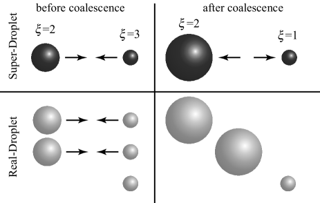
Figure 1: Schematic view of the coalescence of super-droplets. Two super-droplets with multiplicity $2$ and $3$ undergo coalescence (upper left). This represents the coalescence of two droplet pairs (lower left and right). As a result the super-droplet with multiplicity $2$ becomes larger and the multiplicity of the other super-droplet decreases $3\to 1$ (upper right).

Below is the complete definition of how a pair of super-droplets $(j,k)$ change their state after they coalesce:

1. if $\xi_{j}\neq\xi_{k}$, we can choose $\xi_{j}>\xi_{k}$ without losing generality, and

   $$\xi^{\prime}_{j}=\xi_{j}-\xi_{k},\quad\xi^{\prime}_{k}=\xi_{k},$$ (12)

   $$R^{\prime}_{j}=R_{j},\quad R^{\prime}_{k}=(R_{j}^{3}+R_{k}^{3})^{1/3},$$ (13)

   $$M^{\prime}_{j}=M_{j},\quad M^{\prime}_{k}=(M_{j}+M_{k}),$$ (14)

   $$\mathbf{x}^{\prime}_{j}=\mathbf{x}_{j},\quad\mathbf{x}^{\prime}_{k}=\mathbf{x}_{k},$$ (15)

   where the dashed valuables represent the updated value after the coalesce.

2. if $\xi_{j}=\xi_{k}$,

   $$\xi^{\prime}_{j}=[\xi_{j}/2],\quad\xi^{\prime}_{k}=\xi_{j}-[\xi_{j}/2],$$ (16)

   $$R^{\prime}_{j}=R^{\prime}_{k}=\left(R_{j}^{3}+R_{k}^{3}\right)^{1/3},$$ (17)

   $$M^{\prime}_{j}=M^{\prime}_{k}=\left(M_{j}+M_{k}\right),$$ (18)

   $$\mathbf{x}^{\prime}_{j}=\mathbf{x}_{j},\quad\mathbf{x}^{\prime}_{k}=\mathbf{x}_{k},$$ (19)

   where Gauss’ symbol $[b]$ is the greatest integer that is less than or equal to the real number $b$.

Note here that in the case $\xi_{j}=\xi_{k}$, no droplets will be left after the coalescence because all $\xi_{j}$ number of droplets contribute to the coalescence. Thus, we divide the resulting $\xi_{j}$ number of droplets into two super-droplets.

This definition of super-droplet coalescence possesses a favorable property that the number of super-droplets is unchanged in most cases though the number of droplets always decreases. The number of super-droplets is decreased through the coalescence only when $\xi_{j}=\xi_{k}=1$, i.e., both super-droplets are droplets. This results in $\xi^{\prime}_{j}=0$ and $\xi^{\prime}_{k}=1$, and we remove the super-droplet $j$ out of the system. Because the number of super-droplets corresponds to the accuracy of SDM, the number conservation of super-droplets suggests the flexible response of SDM to the drastic change of the number of droplets.

Having defined how a pair of super-droplets coalesces, we turn to determine the probability that the coalescence occurs. If we require the consistency of the expectation value, the probability is determined as the following.

$$\begin{split}P_{jk}^{(s)}=&\max(\xi_{j},\xi_{k})P_{jk}\\ =&\mbox{probability that super-droplet $j$ and $k$ }\\ &\mbox{inside a small region $\Delta V$ will coalesce }\\ &\mbox{in a short time interval $(t,t+\Delta t_{c})$.}\end{split}$$ (20)

Indeed, we can confirm that the expectation value is identical to that of the primitive model (the real world). The super-droplet $j$ represents $\xi_{j}$ droplets with attribute $\mathbf{a}_{j}$ and the super-droplet $k$ represents $\xi_{k}$ droplets with attribute $\mathbf{a}_{k}$. In terms of the real world, this corresponds to the situation that there are $\xi_{j}\xi_{k}$ droplet pairs which have the possibility to coalesce with probability $P_{jk}$. Thus, the number of droplet pairs which will coalescence follows the binomial distribution with $\xi_{j}\xi_{k}$ trials and success probability $P_{jk}$. Thus, in the real world, the expectation value of the number of coalesced pairs is $\xi_{j}\xi_{k}P_{jk}$. On the other hand, in the super-droplet world, a coalescence of the super-droplets $j$ and $k$ represents the coalescence of $\min(\xi_{j},\xi_{k})$ pairs of droplets with attribute $\mathbf{a}_{j}$ and $\mathbf{a}_{k}$. Thus, the coalescence of the super-droplets $j$ and $k$ is expected to represent $\min(\xi_{j},\xi_{k})P_{jk}^{(s)}=\min(\xi_{j},\xi_{k})\max(\xi_{j},\xi_{k})P_{jk}=\xi_{j}\xi_{k}P_{jk}$ coalescences of droplet pairs, which is identical to the value of the real world. It is worth noticing here that the variance in the super-droplet world becomes larger than that of the real world. In the real world, the variance of the number of coalesced pairs is $\xi_{j}\xi_{k}P_{jk}(1-P_{jk})\simeq\xi_{j}\xi_{k}P_{jk}=:V_{r}$ (Poisson distribution limit). In the super-droplet world, the variance is $\{\min(\xi_{j},\xi_{k})\}^{2}P_{jk}^{(s)}-\{\xi_{j}\xi_{k}P_{jk}\}^{2}\simeq\min(\xi_{j},\xi_{k})V_{r}$, which is $\min(\xi_{j},\xi_{k})$ times larger than that of the real world.

We have defined the cloud microphysics of super-droplets. If all the multiplicity $\xi_{i}=1$ then our model is equivalent to the primitive model. Thus, we can change the accuracy of our model by changing the initial distribution of multiplicity $\{\xi_{i}(t=0)\}$, or equivalently, the initial number of super-droplets $N_{s}(t=0)$. If the convergence to the primitive model is rapid, we can say that the use of SDM is beneficial.

The definition of the coalescence process of super-droplets is still theoretical and we have to do numerical simulation on this model somehow. In Sec. 5.1.3, we will develop a Monte Carlo scheme for the stochastic coalescence, which can simulate the coalescence process of super-droplets efficiently.

4.2 Cloud dynamics of Super-Droplet Method

For the cloud dynamics of SDM, we can also apply the non-hydrostatic model (5)-(9). Note here that we have to evaluate the source terms from microphysics (10) and (11) not by the droplets but by the super-droplets:

$$\rho_{w}(\mathbf{x},t)=\sum_{i=1}^{N_{s}}\xi_{i}m_{i}(t)\delta^{3}(\mathbf{x}-\mathbf{x}_{i}(t)),$$ (21)

$$S_{v}(\mathbf{x},t):=\frac{-1}{\rho(\mathbf{x},t)}\sum_{i=1}^{N_{s}}\xi_{i}\frac{dm_{i}(t)}{dt}\delta^{3}(\mathbf{x}-\mathbf{x}_{i}(t)).$$ (22)

5 Super-Droplet Method: numerical implementation

The model developed in the previous section is still theoretical. In this section, we propose a numerical simulation scheme, in which we solve the individual processes independently in different time steps, instead of solving the whole equations at once. In particular, a novel Monte Carlo scheme for the stochastic coalescence process is developed and validated.

5.1 How to simulate cloud microphysics

5.1.1 Motion of super-droplets

Let $\Delta t_{m}$ be the time step to simulate this process. After evaluating the terminal velocity $\mathbf{v}_{i}(t)=\mathbf{U}_{i}^{*}-\hat{\mathbf{z}}v_{\infty}(R_{i}(t))$, we can update the position as $\mathbf{x}_{i}(t+\Delta t_{m})=\mathbf{x}_{i}(t)+\Delta t_{m}\mathbf{v}_{i}(t)$. Here, $\mathbf{U}_{i}^{*}$ is the wind velocity at the super-droplet position $\mathbf{x}_{i}(t)$. As we will see in Sec. 5.2, we use a regular grid $\mathbf{x}_{lmn}$ for the spatial discretization of the fluid field variables. Let us evaluate $\mathbf{U}_{i}^{*}$ by the linear interpolation of the current wind-velocity field $\mathbf{U}(\mathbf{x}_{lmn},t)$.

5.1.2 Condensation/evaporation of super-droplets

Let $\Delta t_{g}$ be the time step to simulate this process. Because the time scale of condensation/evaporation can be much faster than $\Delta t_{g}$, we adopt the implicit Euler discretization scheme for the numerical simulation of (2), yielding

$$\frac{R_{i}^{2}(t+\Delta t_{g})-R_{i}^{2}(t)}{2\Delta t_{g}}\\ =\frac{(S_{i}^{*}-1)-\frac{a(T_{i}^{*})}{R_{i}(t+\Delta t_{g})}+\frac{b(M_{i}(t))}{R_{i}^{3}(t+\Delta t_{g})}}{F_{k}(T_{i}^{*})+F_{d}(T_{i}^{*})},$$

where $S_{i}^{*}$ and $T_{i}^{*}$ are the ambient saturation ratio and the temperature at the super-droplet position $\mathbf{x}_{i}(t)$, which are evaluated by the fluid variables $q_{v}(\mathbf{x}_{lmn},t)$, $\theta(\mathbf{x}_{lmn},t)$, and $\rho(\mathbf{x}_{lmn},t)$, applying interpolation. It may be not possible to determine analytically the next step value $R_{i}(t+\Delta t_{g})$ from the current value $R_{i}(t)$. Hence, we adopt the Newton-Raphson scheme to evaluate $R_{i}(t+\Delta t_{g})$. After evaluating $R_{i}(t+\Delta t_{g})$ for all the super-droplets $i$, we will update the mixing ratio of vapor and potential temperature to $q_{v}(\mathbf{x}_{lmn},t+\Delta t_{g})$ and $\theta(\mathbf{x}_{lmn},t+\Delta t_{g})$. Please refer to Sec. 5.2 for the detail.

5.1.3 Monte Carlo scheme for the coalescence of super-droplets

Let $\Delta t_{c}$ be the time step to simulate this process. Let us introduce a grid which covers the entire real-space for our simulation. We can choose any kind of grid - which may be unstructured - but the volume of each cell must be small enough that the super-droplets are well-mixed inside the cell and the coalescence occurs according to the probability (20) in each cell. Let us make a list of super-droplets in a certain cell at time $t$: $I:=\{i_{1},i_{2},\dots,i_{n_{s}}\}$, where $n_{s}$ is the total number of super-droplets in the cell. Then, by definition, each pair of super-droplets $(j,k)\in I^{2}$, $j\neq k$, coalesces with probability $P_{jk}^{(s)}$ within the short time interval $(t,t+\Delta t_{c})$. Note that $P_{jk}^{(s)}\ll 1$ if $\Delta t_{c}$ is small. We have to examine all the possible pairs $(j,k)$ to know the random realization at the time $t+\Delta t_{c}$. However, this yields computational cost $O(n_{s}^{2})$ and this is not efficient. Instead, we propose a novel Monte Carlo scheme which leads us to $O(n_{s})$ cost in computation.

Let $L:=\{(j_{1},k_{1}),(j_{2},k_{2}),\dots,(j_{[n_{s}/2]},k_{[n_{s}/2]})\}$ be a list of $[n_{s}/2]$ randomly generated, non-overlapping pairs. Non-overlapping means that no super-droplet belongs to more than one pair. This list can be made by generating a random permutation of $I$ and make pairs from the front, which cost $O(n_{s})$ in computation (see Appendix A). By examining only these $[n_{s}/2]$ pairs instead of the whole possible $n_{s}(n_{s}-1)/2$ pairs, the cost will be $O(n_{s})$. In compensation for this simplification, the coalescence probability is divided by the decreasing ratio of pair number, and the corrected, scaled up probability for the $\alpha$th pair is obtained as

$$p_{\alpha}:=P_{j_{\alpha}k_{\alpha}}^{(s)}\frac{n_{s}(n_{s}-1)}{2}\Bigm{/}\left[\frac{n_{s}}{2}\right],\;\;\;\alpha=1,2,\dots,\left[\frac{n_{s}}{2}\right].$$

This may be justified if the following relation holds good,

$$\begin{split}\sum_{\alpha=1}^{[n_{s}/2]}\min(\xi_{j_{\alpha}},\xi_{k_{\alpha}})p_{\alpha}&\simeq\frac{1}{2}\operatorname*{\sum\sum}_{j,k,j\neq k}\min(\xi_{j},\xi_{k})P^{(s)}_{jk}\\ &=\frac{1}{2}\operatorname*{\sum\sum}_{j,k,j\neq k}\xi_{j}\xi_{k}P_{jk},\end{split}$$

which represent the consistency of the expectation number of coalesced droplet pairs in this cell.

Based on the above idea, below is the complete procedure of our Monte Carlo scheme to obtain one of the stochastic realizations in a certain cell at time $t+\Delta t_{c}$ from the sate of super-droplets at time $t$.

1. Make the super-droplet list at time $t$ in this certain cell: $I=\{i_{1},i_{2},\dots,i_{n_{s}}\}$.

2. Make the $[n_{s}/2]$ candidate-pairs $L=\{(j_{1},k_{1}),(j_{2},k_{2}),\dots,(j_{[n_{s}/2]},k_{[n_{s}/2]})\}$ from the random permutation of $I$ (see Appendix A for detail).

3. For each pair of super-droplets $(j_{\alpha},k_{\alpha})\in L$, generate a uniform random number $\phi_{\alpha}\in(0,1)$. Then, evaluate

   $$\gamma_{\alpha}:=\begin{cases}[p_{\alpha}]+1&\text{if $\phi_{\alpha}<p_{\alpha}-[p_{\alpha}]$}\\ [p_{\alpha}]&\text{if $\phi_{\alpha}\geq p_{\alpha}-[p_{\alpha}]$}\end{cases}$$

4. If $\gamma_{\alpha}=0$, the $\alpha$th pair $(j_{\alpha},k_{\alpha})$ is updated to $t+\Delta t_{c}$ without changing their state.

5. If $\gamma_{\alpha}\neq 0$, choose $\xi_{j_{\alpha}}\geq\xi_{k_{\alpha}}$ without losing generality and evaluate $\tilde{\gamma}_{\alpha}:=\min(\gamma_{\alpha},[\xi_{j_{\alpha}}/\xi_{k_{\alpha}}])$.

   1. if $\xi_{j_{\alpha}}-\tilde{\gamma}_{\alpha}\xi_{k_{\alpha}}>0$,

      $$\xi^{\prime}_{j_{\alpha}}=\xi_{j_{\alpha}}-\tilde{\gamma}_{\alpha}\xi_{k_{\alpha}},\quad\xi^{\prime}_{k_{\alpha}}=\xi_{k_{\alpha}},$$

      $$R^{\prime}_{j_{\alpha}}=R_{j_{\alpha}},\quad R^{\prime}_{k_{\alpha}}=(\tilde{\gamma}_{\alpha}R_{j_{\alpha}}^{3}+R_{k_{\alpha}}^{3})^{1/3},$$

      $$M^{\prime}_{j_{\alpha}}=M_{j_{\alpha}},\quad M^{\prime}_{k_{\alpha}}=(\tilde{\gamma}_{\alpha}M_{j_{\alpha}}+M_{k_{\alpha}}),$$

      $$\mathbf{x}^{\prime}_{j_{\alpha}}=\mathbf{x}_{j_{\alpha}},\quad\mathbf{x}^{\prime}_{k_{\alpha}}=\mathbf{x}_{k_{\alpha}},$$

   2. If $\xi_{j_{\alpha}}-\tilde{\gamma}_{\alpha}\xi_{k_{\alpha}}=0$, i.e., $\tilde{\gamma}_{\alpha}=\xi_{j_{\alpha}}/\xi_{k_{\alpha}}=[\xi_{j_{\alpha}}/\xi_{k_{\alpha}}]\leq\gamma_{\alpha}$,

      $$\xi^{\prime}_{j_{\alpha}}=[\xi_{k_{\alpha}}/2],\quad\xi^{\prime}_{k_{\alpha}}=\xi_{k_{\alpha}}-[\xi_{k_{\alpha}}/2],$$

      $$R^{\prime}_{j_{\alpha}}=R^{\prime}_{k_{\alpha}}=\left(\tilde{\gamma}_{\alpha}R_{j_{\alpha}}^{3}+R_{k_{\alpha}}^{3}\right)^{1/3},$$

      $$M^{\prime}_{j_{\alpha}}=M^{\prime}_{k_{\alpha}}=\left(\tilde{\gamma}_{\alpha}M_{j_{\alpha}}+M_{k_{\alpha}}\right),$$

      $$\mathbf{x}^{\prime}_{j_{\alpha}}=\mathbf{x}_{j_{\alpha}},\quad\mathbf{x}^{\prime}_{k_{\alpha}}=\mathbf{x}_{k_{\alpha}}.$$

      If $\xi^{\prime}_{j_{\alpha}}=0$, the super-droplet $j_{\alpha}$ is removed out of the system.

Our Monte Carlo scheme numerically solves the stochastic coalescence process of super-droplets defined in Sec. 4.1.4. We reduced the candidate pairs using a random permutation technique to achieve the computational cost $O(n_{s})$. Further extension are introduced in our Monte Carlo scheme to deal with multiple coalescence. The integer $\gamma_{\alpha}$ represents how many times the pair $(j_{\alpha},k_{\alpha})$ will coalesce, and $\tilde{\gamma}_{\alpha}$ is the restricted value of $\gamma_{\alpha}$ by its maximum value $[\xi_{j_{\alpha}}/\xi_{k_{\alpha}}]$. Primarily, $p_{\alpha}$ must be smaller than $1$ because $p_{\alpha}$ represents a probability, thus $\gamma_{\alpha}$ should be either $0$ or $1$. However, if we take $\Delta t_{c}$ too much larger, $p_{\alpha}$ may become larger than $1$. Though the situation $\gamma_{\alpha}>1$ is not consistent with the fundamental premise of our theory, we formulate our Monte Carlo scheme to cope with this situation so that SDM robustly well-approximates the primitive model irrespective of the choice of $\Delta t_{c}$.

Alternatively, the most rigorous selection criteria of the simulation time step for the coalescence process $\Delta t_{c}$ is that $p_{\alpha}\ll 1$ holds good for all the candidate pairs $\alpha$. Let us estimate $\Delta t_{c}$ very roughly. The typical number density and radius of small cloud droplets are $10^{9}~{}\mathrm{m}^{-3}$ and $R=10~{}\mu\mathrm{m}$. The typical terminal velocity of a rain droplet is $1~{}\mathrm{m~{}s^{-1}}$. Then, we may roughly evaluate $p_{\alpha}$ as follows.

$$\begin{split}p_{\alpha}&\simeq n_{s}P_{j_{\alpha}k_{\alpha}}^{(s)}\\ &=\frac{n_{s}\max{(\xi_{j_{\alpha}},\xi_{k_{\alpha}})}}{\Delta V}E\pi(R_{j_{\alpha}}+R_{k_{\alpha}})^{2}\lvert\mathbf{v}_{j_{\alpha}}-\mathbf{v}_{k_{\alpha}}\rvert\Delta t_{c}\\ &\simeq 10^{9}\text{m}^{-3}\cdot 1\cdot\pi(2\times 10^{-5}\text{m})^{2}\cdot 1~{}\mathrm{m~{}s^{-1}}\cdot\Delta t_{c}\\ &=(0.4\pi~{}\mathrm{s^{-1}})\Delta t_{c}.\end{split}$$

Because $p_{\alpha}<1$ should be satisfied, we can estimate that $\Delta t_{c}<1/(0.4\pi~{}\mathrm{s^{-1}})\simeq 0.8~{}\mathrm{s}$. It is worth noticing here, that our estimation is independent of the number of super-droplets $n_{s}$ and the volume of the coalescence cell $\Delta V$.

5.1.4 Validation of our Monte Carlo scheme

In this section, we validate our Monte Carlo scheme for the stochastic coalescence process by confirming that the numerical results agree well with the solution of a SCE.

The super-droplets in this section undergo only the coalescence process, which will be simulated by our Monte Carlo scheme. The super-droplets have velocities, but do not move out of the coalescence cell, nor do they undergo condensation/evaporation. The equivalent radius of water $R_{i}$ is the only attribute. The corresponding SCE for this extreme case can be derived as

$$\begin{split}\frac{\partial n(X,t)}{\partial t}=\;&\frac{1}{2}\int_{0}^{X}dX^{\prime}n(X^{\prime})n(X^{\prime\prime})K(X^{\prime},X^{\prime\prime})\\ &-n(X)\int_{0}^{\infty}dX^{\prime}n(X^{\prime})K(X,X^{\prime}),\end{split}$$ (23)

where $n(X,t)$ is the number density of droplets, $X=(4\pi/3)R^{3}$ is the water volume of droplet, $K$ is the coalescence kernel defined in (3), and $X^{\prime\prime}:=X-X^{\prime}$.

To compare the simulation result, we have to reconstruct the number density distribution $n(X,t)$ from the data of super-droplets $\{(\xi_{i},R_{i})\}$. There are several ways to do this, but we adopt the kernel density estimate method with Gaussian kernel (Terrell and Scott, 1992). Some brief discussions on the application of the kernel density estimate method to SDM is also developed in Sec. 7.2. It is convenient to plot the results by the mass density function over $\ln R$, which is defined by $g(\ln R)d\ln R:=\rho_{\mathrm{liq}}Xn(X)dX$. The corresponding estimator function $\tilde{g}(\ln R)$ becomes,

$$\begin{split}\tilde{g}(\ln R)&:=\frac{1}{\Delta V}\sum_{i=1}^{N_{s}}\xi_{i}m_{i}W_{\sigma}(\ln R-\ln R_{i}),\\ W_{\sigma}(Y)&:=\frac{1}{\sqrt{2\pi}\sigma}\exp{\left(-Y^{2}/2\sigma^{2}\right)}.\\ \end{split}$$

Here, $\Delta V$ is the volume of the coalescence cell, and $\sigma=\sigma_{0}N_{s}^{-1/5}$ with some constant $\sigma_{0}$. Theoretically, the most efficient choice of $\sigma_{0}$ is estimated as $\sigma_{0}=(2\sqrt{\pi}\Delta V^{2}\int g^{\prime\prime 2}d\ln R/M_{\mathrm{tot}}N_{r})^{-1/5}$, where $M_{\mathrm{tot}}$ is the total mass of liquid water. Because $g$ itself is the function under estimation, we have to estimate also $\sigma_{0}$ from the data of super-droplets to find the maximum likelihood estimator function $\tilde{g}$, but in this paper we simply choose $\sigma_{0}$ empirically.

We have to give an explicit form of the coalescence kernel $K(R_{j},R_{k})$ in (3) to determine the dynamics. For Golovin’s kernel $K(R_{j},R_{k})=b(X_{j}+X_{k})$, we have the analytic solution of the SCE (23) (Golovin, 1963) though this choice of coalescence kernel is not realistic. The result of our comparison simulation for Golovin’s kernel is shown in Fig. 2a. We set $b=1.5\times 10^{3}~{}\mathrm{s^{-1}}$. We need only use one big coalescence cell, the volume of which is chosen as $\Delta V=10^{6}~{}\mathrm{m}^{3}$. The time step is fixed as $\Delta t_{c}=1.0~{}\mathrm{s}$. The initial number density of droplets is set to be $n_{0}=2^{23}~{}\mathrm{m}^{-3}$. The initial size distribution of the droplets follows an exponential distribution of the droplet volume $X_{i}$ which is determined by the probability density $p(X_{i})=(1/X_{0})\exp{\left(-X_{i}/X_{0}\right)}$, $X_{0}=(4\pi/3)R_{0}^{3}$, $R_{0}=30.531\times 10^{-6}~{}\mathrm{m}$. This setting results in the total amount of liquid water $1.0~{}\mathrm{g~{}m^{-3}}$. The initial number of super-droplet $N_{s}$ is changed as the simulation parameter. The initial multiplicity $\xi_{i}$ is determined by the equality $\xi_{i}=n_{0}\Delta V/N_{s}$. $\sigma_{0}$ is fixed as $\sigma_{0}=0.62$.

Figures 2b and 2c show the results for the case of the so-called hydrodynamic kernel, which is a much more realistic coalescence kernel, defined by (3) and (4). The same coalescence efficiency $E(R_{j},R_{k})$ is adopted as described in Seeßelberg et al. (1996) and Bott (1998): For small droplets the dataset of Davis (1972) and Jonas (1972) is used, and for large droplets the dataset of Hall (1980) is used. Because the analytic solution is not available for hydrodynamic kernel, we generated the reference solution numerically using the Exponential Flux Method (EFM) developed by Bott (1998, 2000). A logarithmically equidistant radius grid is used in EFM. We adopted 1000 bins ranging from 0.62 $\mu$m to 6.34 cm. The time step was set to 0.1 s. These parameter settings provide a sufficiently accurate numerical solution of the SCE (23). In Fig. 2b, simulation settings are the same as in case (a) except for the coalescence kernel. In Fig. 2c we changed the initial size distribution by reducing $R_{0}$ to one-third, i.e., $R_{0}=10.177\times 10^{-6}~{}\mathrm{m}$, and increased the initial number density of droplets as $n_{0}=3^{3}\cdot 2^{23}~{}\mathrm{m}^{-3}$. Consequently, the total amount of liquid water $1.0~{}\mathrm{g~{}m^{-3}}$ is unchanged from the case (b). $\Delta t_{c}=0.1~{}\mathrm{s}$ and $\sigma_{0}=1.5$ for the case (c).

In case (a) and (b), we can see that the result of SDM with $N_{s}=2^{13}$ agrees fairly well with the solution of SCE (23), and is much improved when $N_{s}=2^{17}$. However, case (c) is not so good as the previous two cases. Even $N_{s}=2^{17}$ is not good and we need $N_{s}=2^{21}$ for good agreement. This situation reveals a typical weak point of SDM. The initial size of the droplets is comparatively small and coalescence hardly occurs. We can see that the thick solid line at $t=1200~{}\mathrm{s}$ is not so changed from the initial distribution. However, once a few big droplets are created, then the coalescence process is abruptly accelerated. Accordingly, for an accurate prediction, we have to resolve the right tail of the distribution at the time $t=1200~{}\mathrm{s}$. However, the existence probability of super-droplets is very low for this region and sampling error occurs if the number of super-droplets $N_{s}$ is not sufficient. As a result, we need many more super-droplets for the case (c) compared to that of (a) and (b). For practical applications to cloud formation, this fact would not impose severe restrictions on SDM because the condensation/evaporation process dominates the growth of small droplets in such cases like (c).

Anyway, we have confirmed that SDM reproduces the solution of the SCE (23) if the number of super-droplets $N_{s}$ is sufficiently large. These results support the validity of our Monte Carlo scheme for the stochastic coalescence.

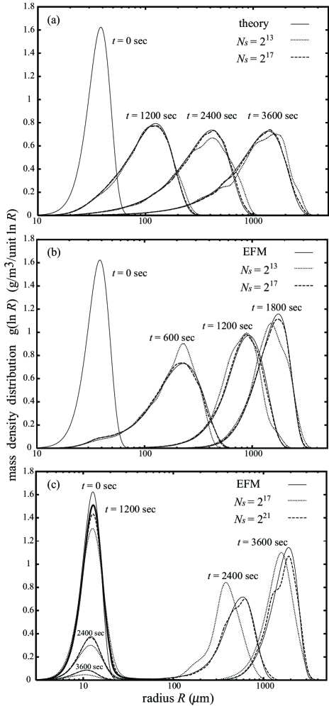
Figure 2: Time evolution of the mass density distribution $g(\ln R,t)$, which is numerically obtained by the Monte Carlo scheme of SDM. (a): The case of Golovin’s kernel. The solid line represents the analytic solution of the SCE (23). (b) and (c): The case of hydrodynamic kernel. The solid line represents the approximate solution of the SCE (23), which is numerically obtained by EFM. In each case, we can see that the result of SDM agrees fairly well with solution of the SCE (23) when the number of super-droplets $N_{s}$ is sufficiently large. $\Delta t_{c}=1.0~{}\mathrm{s}$ for (a) and (b), and $\Delta t_{c}=0.1~{}\mathrm{s}$ for (c).

5.2 How to simulate cloud dynamics

Let $\Delta t_{f}$ be the time step to simulate this process. Let us introduce a regular grid for the spatial discretization of the fluid field variables, and let $\mathbf{x}_{lmn}$ be the position coordinate of the grid point $(l,m,n)$. Then, we can adopt the 4th-order Runge-Kutta scheme for the time derivative, the second-order central difference scheme for the spatial derivatives, with artificial viscosity to stabilize the numerical instability, to simulate (5)-(9).

Here, the cloud microphysics processes exert an influence on the cloud dynamics through the source terms (21) and (22). While we calculate the momentum coupling related to (21) in the fluid time step $\Delta t_{f}$, we calculate the vapor and latent heat coupling related to (22) in the condensation/evaporation time step $\Delta t_{g}$, in the following manner.

Every time, before updating the fluid variables in the $\Delta t_{f}$ time step, we evaluate the momentum coupling term (21) from the current state of the super-droplets. Here, (21) must be evaluated on the numerical grid point $\mathbf{x}_{lmn}$. Generally, by introducing an appropriately chosen coarsening function $w(\mathbf{x})$, it can be evaluated as

$$\begin{split}\rho_{w}(\mathbf{x}_{lmn},t)&=\int w(\mathbf{x}_{lmn}-\mathbf{x})\rho_{w}(\mathbf{x},t)d^{3}x\\ &=\sum_{i=1}^{N_{s}}\xi_{i}m_{i}(t)w(\mathbf{x}_{lmn}-\mathbf{x}_{i}(t)).\end{split}$$

Here $w$ satisfies $\int w(\mathbf{x})d^{3}x=1$, and would be a piecewise linear, localized function with length-scale comparable to the grid width. Our simplest choice is to share each super-droplet by the 8 adjacent grid points at the corner of the cell, then $w(\mathbf{x})=1/8\Delta V$ inside the cube with volume $8\Delta V$, and $w(\mathbf{x})=0$ outside the cube. Then, using this $\rho_{w}(\mathbf{x}_{lmn},t)$, we perform the 4th-order Runge-Kutta scheme to update the fluid variables to the time $t+\Delta t_{f}$.

On the other hand, we calculate the increase and decrease of vapor and potential temperature through (22) after we have calculated the condensation/evaporation of super-droplets in the time step $\Delta t_{g}$ (see also Sec. 5.1.2). Similarly to $\rho_{w}(\mathbf{x}_{lmn},t)$, $S_{v}$ on the grid point $\mathbf{x}_{lmn}$ is evaluated as

$$S_{v}(\mathbf{x}_{lmn},t)=\frac{-1}{\rho(\mathbf{x}_{lmn},t)}\\ \times\sum_{i=1}^{N_{s}}\xi_{i}\frac{m_{i}(t+\Delta t_{g})-m_{i}(t)}{\Delta t_{g}}w(\mathbf{x}_{lmn}-\mathbf{x}_{i}(t)).$$

Then, the mixing ration of vapor and the potential temperature are updated as

$$\theta(\mathbf{x}_{lmn},t+\Delta t_{g})=\theta(\mathbf{x}_{lmn},t)-\Delta t_{g}\frac{LS_{v}(\mathbf{x}_{lmn},t)}{c_{p}\Pi(\mathbf{x}_{lmn},t)},$$

$$q_{v}(\mathbf{x}_{lmn},t+\Delta t_{g})=q_{v}(\mathbf{x}_{lmn},t)+\Delta t_{g}S_{v}(\mathbf{x}_{lmn},t).$$

The way how to simulate the primitive model using the SDM has now been obtained completely.

6 Proof of concept

A simple test of a shallow maritime cumulus formation initiated by a warm bubble is presented in this section to evaluate the behavior of our model.

The simulation domain is 2-dimensional ($x$-$z$), 12.8 km in the horizontal direction and 5.12 km in the vertical direction. Initially, a humid but not saturated atmosphere is stratified, which is almost absolutely unstable under 2 km in altitude. There is a temperature inversion layer above 2 km. The equations below determine the initial base sounding of the atmosphere.

$$\mathbf{U}(\mathbf{x},t=0)=0,$$

$$T(x,z=0,t=0)=305.0~{}\mathrm{K},$$

$$P(x,z=0,t=0)=101325~{}\mathrm{Pa},$$

$$\frac{\partial T}{\partial z}=\begin{cases}-9.5~{}\mathrm{K~{}km^{-1}}&\text{if $z<2.0~{}\mathrm{km}$},\\ +3.0~{}\mathrm{K~{}km^{-1}}&\text{if $z\geq 2.0~{}\mathrm{km}$},\end{cases}$$

$$q_{v}(\mathbf{x},t=0)=0.022\exp{\left[-\left\{\frac{(z+200.0~{}\mathrm{m})}{2000.0~{}\mathrm{m}}\right\}^{2}\right]}.$$

The upper and lower boundaries are fixed to their initial values and the horizontal boundary is periodic. A warm bubble is inserted at the center of the horizontal axis according to the equation below.

$$\theta(\mathbf{x},t=0)=\theta_{b}(\mathbf{x},t=0)+1.0~{}\mathrm{K}\\ \times\exp{\left[-\left\{\frac{(z-500.0~{}\mathrm{m})}{400.0~{}\mathrm{m}}\right\}^{2}-\left\{\frac{(x-6.4~{}\mathrm{km})}{1200.0~{}\mathrm{m}}\right\}^{2}\right]},$$

where $\theta_{b}(\mathbf{x},t=0)$ is the base state of potential temperature.

We simulate the cloud dynamics according to the non-hydrostatic model introduced in Sec. 2.2 with the numerical schemes proposed in Sec. 5.2. We use a regular grid with the mesh size $\Delta x=3.125~{}\mathrm{m}$ and $\Delta z=4.0~{}\mathrm{m}$. The time step is $\Delta t_{f}=0.0125~{}\mathrm{s}$. We set the artificial viscosity $\nu=\kappa=1.5625~{}\mathrm{m^{2}~{}s^{-1}}$.

Initially, NaCl aerosols are uniformly distributed in space with number density $1.0\times 10^{7}~{}\mathrm{m}^{-3}$. The solute mass $M_{i}(t=0)$ has an exponential distribution given by the probability density $p(M_{i})=(1/M_{0})\exp{(-M_{i}/M_{0})}$, $M_{0}=1.0\times 10^{-16}~{}\mathrm{g}$. Because it is unsaturated at the beginning, the growth equation (2) has a stable and steady solution, which is adopted as the initial value of the equivalent radius of water $R_{i}(t=0)$. The coalescence efficiency used in Sec. 5.1.4 is also adopted to this simulation.

For the numerical simulation of the microphysical processes, we also use the numerical schemes proposed in Sec. 5. The same grid as that of the non-hydrostatic model is adopted for our Monte Carlo scheme. Initially, the super-droplets are uniformly distributed in space and the number density is chosen as $64$ per cell. We consider that we have a single cell in the $y$-direction of dimension $100~{}\mathrm{m}$, then the number density of super-droplets is equivalent to $64/\mathrm{cell}=5.12\times 10^{-2}~{}\mathrm{m}^{-3}$. For the super-droplets, we impose a common initial multiplicity, which value is determined by $\xi_{i}(t=0)=~{}\text{INT}(1.0\times 10^{7}/5.12\times 10^{-2})=195312500$. The time steps are $\Delta t_{m}=\Delta t_{g}=\Delta t_{c}=1.0~{}\mathrm{s}$.

Cloud started to form at about $8$ min and began to rain at about $20$ min. After raining for half an hour, the cloud remained for a while but finally disappeared at about $90$ min. The amount of precipitation is about $1$ mm in total. Figure 3 is a snapshot at time $1620$ s. We plot the super-droplets with the color and the alpha transparency which are determined by their radius $R_{i}$ and multiplicity $\xi_{i}$. The color map is indicated in the figure and the alpha value is determined by $\alpha_{i}=1.0\times 10^{-5}(R_{i}/10^{-3}~{}\mathrm{m})^{2}~{}\xi_{i}$, which is proportional to $R_{i}^{2}\xi_{i}$. We can see that the turbulent-like structures inside the cloud are resolved in our simulation. Note that there are super-droplets also in the black region, but it is not depicted in this figure because the water amount contained in the super-droplets is very low; these super-droplets are aerosols.

To perform an accurate simulation, the number of super-droplets $N_{s}$ must be sufficiently large. However, it is not so easy to determine the optimal number of super-droplets to be used. A lower bound is to use about $100$ super-droplets per fluid cell, otherwise the source terms $\rho_{w}(\mathrm{x}_{lmn},t)$ and $S_{v}(\mathrm{x}_{lmn},t)$ would be not smooth enough in space compared to the fluid variables. An upper bound is to use about $100,000$ super-droplets for each coalescence cell if the number of attributes $d=1$. Then the droplet size distribution in each coalescence cell can be fully resolved, as we have already discussed in Sec. 5.1.4. In our simulation, we used only $64$ super-droplets for each coalescence cell, nevertheless we found that the overall behavior, such as the cloud shape and the lifetime, fairly well converged. Further analyses have to be carried out to confirm the convergence of our simulation by checking the detailed structures of the cloud, such as the droplet size distribution and the aerosol size distribution.

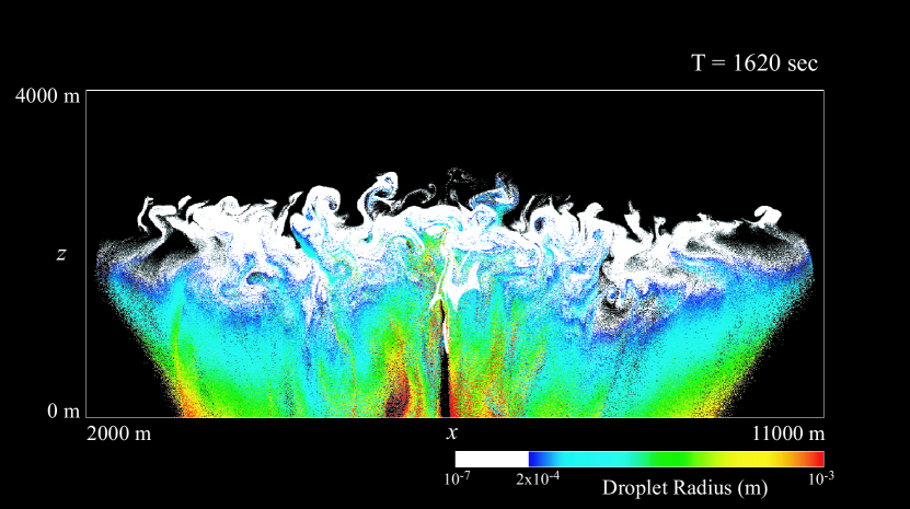
Figure 3: Shallow maritime cumulus formation initiated by a warm bubble simulated by SDM. This is a snapshot at time $1620$ s. The super-droplets are plotted with the color and the alpha transparency which are determined by their radius $R_{i}$ and multiplicity $\xi_{i}$. The color map is indicated in the figure and the alpha value is determined by $\alpha_{i}=1.0\times 10^{-5}(R_{i}/10^{-3}~{}\mathrm{m})^{2}~{}\xi_{i}$, which is proportional to $R_{i}^{2}\xi_{i}$. We can see that the turbulent like structures inside the cloud is resolved in our simulation. Note that super-droplets are also in the black region, but they are not depicted in this figure because they are regarded as aerosols.

7 Future Direction

7.1 Extension of Super-Droplet Method

The model we developed in Sec. 4 and 5 was only for warm rain with only one soluble substance as the aerosol. However, it is very conceivable that we can extend SDM to incorporate various cloud microphysical processes, such as, several sorts of soluble/insoluble aerosols, their chemical reactions, several types of ice crystals, electrification, and the breakup of droplets. Here, the possible extensions of the method is briefly discussed.

For this purpose, let us generalize the definition of attributes as $\mathbf{a}(t)=(a^{(1)},a^{(2)},\dots,a^{(d)})$, where $d$ is the number of independent attributes. Then, we have to construct the time evolution law of attributes that determines the individual dynamics of super-droplets, which can be written as:

$$\frac{d\mathbf{a}_{i}}{dt}=\mathbf{f}(\mathbf{a}_{i},\mathbf{A}(\mathbf{x}_{i})),\quad i=1,2,\dots,N_{s}(t),$$ (24)

where $\mathbf{A}(\mathbf{x}_{i})$ represents the field variable which characterizes the state of the ambient atmosphere. In the case of the primitive model, eq. (24) consists of two equations: the growth equation (2) and the time evolution of solute mass $dM_{i}/dt=0$.

The stochastic coalescence process have to be redefined for our new super-droplets. At first, we have to determine what kind of droplet $\mathbf{a}^{\prime}$ will be created after the coalescence of droplets $\mathbf{a}_{j}$ and $\mathbf{a}_{k}$. Then, the coalescence of super-droplets will be determined similarly to (12)-(19). It is not the case in (15) and (19), but we may also change the position of the super-droplets after the coalescence if necessary. Similar to (3), the coalescence probability for droplets could be evaluated in the form

$$\begin{split}P_{jk}=&C(\mathbf{a}_{j},\mathbf{a}_{k})\frac{\Delta t_{c}}{\Delta V}|\mathbf{v}_{j}-\mathbf{v}_{k}|\\ =&\mbox{probability that droplet $j$ and $k$ }\\ &\mbox{inside a small region $\Delta V$ will coalesce }\\ &\mbox{in a short time interval $(t,t+\Delta t_{c})$,}\end{split}$$ (25)

which in general is a function of the attributes $\mathbf{a}_{j}$ and $\mathbf{a}_{k}$. Then the coalescence probability of super-droplets will be determined by (20).

Incorporating the breakup of droplets to the SDM framework is a remaining problem to be solved. Such a formulation would be desirable that the number of super-droplets do not change after a breakup event, but this is our future task.

In various research areas, many types of particle-based simulation schemes have been developed recently. SDM can be regarded as a sort of Direct Simulation Monte Carlo (DSMC) method, which was initially proposed to simulate the Boltzmann equation for predicting rarefied gas flows (Bird, 1994). In particular, SDM has similarity to the Extended version of the No-Time-Counter (ENTC) method, which was developed by Schmidt and Rutland (2000) for the simulation of spray flows. Though the basic idea of using a computational particle with varying multiplicity is common in both SDM and ENTC, the Monte Carlo procedures to simulate the stochastic coalescence process are different: SDM is using $[n_{s}/2]$ randomly generated, non-overlapping candidate pairs, and allows multiple coalescence for each pair. On the other hand, the ENTC method chooses the candidate pairs randomly from the set of all the possible pairs. The number of candidate-pairs to be sampled varies proportionally to the maximum coalescence probability in the cell. Both the SDM and the ENTC methods result in the computational cost $O(N_{s})$. Presumably, the ENTC method is also applicable to cloud simulations and SDM is applicable to spray simulations, but further verifications are still necessary to compare their capability.

Independently to the work by the present authors, there exist several ongoing studies to construct novel cloud microphysics models employing similar ideas as SDM. Andrejczuk et al. (2008) have developed a particle-based cloud microphysics model, in which they have implemented the ice phase processes and some aerosol chemistry processes. In their paper, the stochastic coalescence process was not incorporated yet, but they are currently developing an original deterministic scheme to calculate the stochastic coalescence process (2008, personal communication). On the other hand, a work employing a probabilistic approach to accelerate the spectral (bin) method is currently in progress by Sato et al. (2008, personal communication).

7.2 Computational cost and accuracy

The possible extension of the SDM has been discussed in the previous section. We can see that once the fundamental equations of the cloud microphysical processes, (24) and (25), are given, we can perform an accurate simulation using the SDM. However, this statement is also true for the spectral (bin) method. Then, which method is computationally more efficient?

To answer this question, we have carried out a simple theoretical analysis to compare the computational cost of the SDM and the spectral (bin) method, which is presented in Appendix B. Here, the costs are evaluated by the amount of the operation count and memory necessary to reproduce the number density distribution of droplets within a certain margin of error.

The assertions must still be verified, but our estimation suggests that the computational cost of SDM could be less demanding than the spectral (bin) method when the number of attributes $d$ is larger than some critical value $d_{c}$. In the case when the attribute-spatial discretization error of the spectral (bin) method is in the range $1\sim 2$, then the critical value $d_{c}$ is estimated to be in the range $2\sim 4$.

Finally, we would like to present some supplemental data on the actual CPU behavior of SDM. In Sec. 5.1.4, we tested our Monte Carlo scheme and compared the results with the spectral (bin) method. In case (b), the FLoating point OPeration (FLOP) count was $2.7~{}\mathrm{G}$ and the memory used was $192~{}\mathrm{MB}$ for $N_{s}=2^{13}$. For $N_{s}=2^{17}$, the FLOP count was $4.2\times 10~{}\mathrm{G}$ and the memory used was $208~{}\mathrm{MB}$. We produced the reference solution by EFM, the spectral (bin) method developed by Bott, using $N_{b}=1000$ bins. For this simulation, the FLOP count was $6.5\times 10^{2}~{}\mathrm{G}$ and the memory used was $80~{}\mathrm{MB}$. Practically, $N_{b}=100$ would be sufficient and in this setting the FLOP count is $7.5~{}\mathrm{G}$ and the memory used is $48~{}\mathrm{MB}$, and we need $13~{}\mathrm{s}$ in wall-clock time to complete this simulation if we use one Intel Pentium 4 CPU $3.20~{}\mathrm{GHz}$.

In Sec. 6 we performed a 2D simulation of a shallow maritime cumulus formation. In this simulation, the FLOP count was $9.3\times 10^{6}~{}\mathrm{G}$ and the memory used was $65~{}\mathrm{GB}$. We used $32$ nodes of the Earth Simulator, using $11$ hours of wall-clock time to complete $2.5$ hours of simulated time, which means that the performance of our calculation was $2.3\times 10^{2}~{}\mathrm{GFLOPS}$ (Giga FLoating point Operations Per Second). This is $11~{}\%$ of the peak performance.

8 Summary and concluding remarks

In this paper, we proposed the SDM as a new approach for the accurate simulation of clouds and precipitation.

The primitive model was introduced at the beginning, which is a detailed microphysics-dynamics coupled warm-cloud model. In this paper the primitive model was regarded as the master framework for describing the behavior of warm clouds. We saw how the traditional methods can simulate the primitive model and what are the problems involved.

Then, we applied the SDM to the primitive model. First, introducing the notion of super-droplets, we derived the basic equations of SDM and discussed the ideas of SDM. Next, a numerical implementation scheme was proposed for each process. In particular, a novel Monte Carlo scheme for the stochastic coalescence process was developed and validated by comparing the numerical results with the solutions of SCE.

To evaluate the behavior of our model, we performed a simple testing simulation of a shallow maritime cumulus formation initiated by a warm bubble. Brief discussions were carried out on the possible extensions of the SDM to incorporate various other cloud microphysical processes. Our theoretical estimation suggested that SDM becomes computationally more efficient than the spectral (bin) method when the number of attributes $d$ becomes larger than some critical value, which we estimate to be in the range $2\sim 4$.

Though several extensions and validations are still necessary, we expect that SDM would be more feasible for the modeling of complicated cloud microphysical processes, and provide us a new approach to the open problems in cloud science, such as cloud and aerosol interactions, cloud-related radiative processes, and the mechanism of thunderstorms and lightning.

The authors are grateful to A. Bott for offering his Fortran program, F. Araki for fruitful discussions, and T. Sato for his continued support. S.S. would like to thank T. Miyoshi, Y. Kawamura, S. Koyama, S. Hirose, H. Nakao, and R. Onishi for valuable comments and encouragement. This work is one of the results of the Earth Simulator project “Development of Multi-scale Coupled Simulation Algorithm.”

Appendix A How to make a random permutation

Let $a^{(n)}=(a^{(n)}_{1},a^{(n)}_{2},\dots,a^{(n)}_{n})$ be a permutation of $I_{n}:=(1,2,\dots,n)$. Let $S_{n}:=\{a^{(n)}\}$ be the set of all the permutation of $I_{n}$. Thus, $S_{n}$ has $n!$ number of elements. Let us define the random permutation of $I_{n}$ by such a permutation $a^{(n)}$ that all the $a^{(n)}\in S_{n}$ occurs with the same probability, i.e., $P(a^{(n)})=1/n!$, $\forall a^{(n)}\in S_{n}$.

We have two propositions. 1) $a^{(1)}=(1)$ is a random permutation of $I_{1}$. 2) We can make a random permutation of $I_{n+1}$ from a random permutation of $I_{n}$ by the following procedure: Let $a^{(n)}$ be a random permutation of $I_{n}$ and choose $m$ from $1,2,\dots,n+1$ randomly. Let $a^{(n+1)}=(a^{(n)},n+1)=(a^{(n)}_{1},\dots,a^{(n)}_{n},n+1)$. If $m\neq n+1$, exchange the value at $m$ and $n+1$, i.e., $a^{(n+1)}_{n+1}=a^{(n)}_{m}$, $a^{(n+1)}_{m}=n+1$. Then, $a^{(n+1)}$ is a random permutation of $I_{n+1}$.

Proposition 1) is obvious and 2) is also easy to prove. For all $a^{(n+1)}\in S_{n+1}$, we can uniquely determine $a^{(n)}\in S_{n}$ which have the possibility to become $a^{(n+1)}$. Indeed, such $a^{(n)}$ is given by $a^{(n)}=(a^{(n+1)}_{1},a^{(n+1)}_{2},\dots,a^{(n+1)}_{m-1},a^{(n+1)}_{n+1},a^{(n+1)}_{m+1},\dots,a^{(n+1)}_{n})$, here $m$ satisfies $a^{(n+1)}_{m}=n+1$. If $m=n+1$, $a^{(n)}_{i}=a^{(n+1)}_{i}$, $i=1,\dots,n$. Then, the probability that $a^{(n+1)}$ occurs is evaluated by $P(a^{(n+1)})=P(a^{(n)})\times 1/(n+1)=1/(n+1)!$.

Consequently, we can make a random permutation of $I_{n}$ with $O(n)$ operations.

Appendix B Estimation of the computational cost of the spectral (bin) method and the SDM

First, let us estimate the computational cost and accuracy of the spectral (bin) method. We have extended SDM in Sec. 7.1, and the corresponding, more general form of SCE can be derived as follows.

$$\frac{\partial n(\mathbf{a},\mathbf{x},t)}{\partial t}+\nabla_{x}\cdot\left\{\mathbf{v}n\right\}+\nabla_{a}\cdot\left\{\mathbf{f}n\right\}=\left(\frac{\partial n}{\partial t}\right)_{c},$$ (26)

$$\begin{split}\left(\frac{\partial n}{\partial t}\right)_{c}:=~{}&\frac{1}{2}\int d^{d}a^{\prime}n(\mathbf{a}^{\prime})n(\mathbf{a}^{\prime\prime})K(\mathbf{a}^{\prime},\mathbf{a}^{\prime\prime})\\ &-n(\mathbf{a})\int d^{d}a^{\prime}n(\mathbf{a}^{\prime})K(\mathbf{a},\mathbf{a}^{\prime}).\end{split}$$

where $n(\mathbf{a},\mathbf{x},t)$ is the number density distribution, $\mathbf{f}$ is defined in (24), and $\mathbf{a}^{\prime\prime}$ is such attribute that will become $\mathbf{a}$ if it coalesces with $\mathbf{a}^{\prime}$. The term $(\partial n/\partial t)_{c}$ corresponds to the ensemble-averaged dynamics of the stochastic coalescence process, and this term is $d$-multiple integral in general because we have to survey all over the $d$-dimensional attribute-space to evaluate the time evolution of the droplet number density at $\mathbf{a}$. Obviously, this term is computationally most expensive. Therefore, to simplify the discussions, we neglect the advection terms in the l.h.s of (26) and focus our attention on the simplified equation $\partial n(\mathbf{a},t)/\partial t=(\partial n/\partial t)_{c}$, which corresponds to the extreme situation that only the stochastic coalescence is taken into account as the microphysical process.

Let $N_{b}$ be the number of bins for each attribute, i.e., the number of grid points used for the discretization of $n(\mathbf{a})$ per attribute. Then, because $\partial n/\partial t=(\partial n/\partial t)_{c}$ is a $d$-multiple integro-differential equation, the operation count and memory required for the computation of spectral (bin) method scales like “$\text{\it operation}\sim N_{b}^{2d}$” and “$\text{\it memory}\sim N_{b}^{d}$.”

To evaluate the accuracy of the spectral (bin) method, let us introduce the Integrated Squared Error (ISE),

$$C=\int d^{d}a\;\left\{n(\mathbf{a})-n_{b}(\mathbf{a})\right\}^{2}.$$ (27)

Here, $n_{b}(\mathbf{a})$ is the approximate solution generated by the spectral (bin) method, and $C$ measure the difference of $n_{b}(\mathbf{a})$ from the exact solution $n(\mathbf{a})$. If the discretization error of the spectral (bin) method is $k$th order in attribute-space, $C$ scales like $C\sim N_{b}^{-2k}$ by definition.

Combining the above mentioned results, we can estimate the scaling of operation count and memory needed for the computation of spectral (bin) method in terms of $C$ as follows,

$$\begin{split}\text{\it operation}&\sim N_{b}^{2d}\sim\left(\frac{1}{\sqrt{C}}\right)^{2d/k},\\ \text{\it memory}&\sim N_{b}^{d}\sim\left(\frac{1}{\sqrt{C}}\right)^{d/k}.\end{split}$$ (28)

Next, let us estimate the computational cost and accuracy of SDM. To compare the result with the spectral (bin) method, we only consider the stochastic coalescence process, and estimate the number density distribution $n(\mathbf{a})$ from the super-droplets $\{(\xi_{i},\mathbf{a}_{i})\mid i=1,2,\dots,N_{s}\}$. For the estimation, we use the kernel density estimation method, which was originally developed to estimate the generating probability distribution from its random sample (Terrell and Scott, 1992).

We use the density estimator function $\tilde{n}(\mathbf{a})$ with Gaussian kernel $W_{\sigma}^{(d)}(\mathbf{a})$, defined by

$$\begin{split}\tilde{n}(\mathbf{a})&:=\sum_{i=1}^{N_{s}}\xi_{i}W_{\sigma}^{(d)}(\mathbf{a}-\mathbf{a}_{i}),\\ W_{\sigma}^{(d)}(\mathbf{a})&:=\frac{1}{(\sqrt{2\pi}\sigma)^{d}}\exp{\left\{-\mathbf{a}^{2}/2\sigma^{2}\right\}}.\end{split}$$ (29)

The error evaluation function corresponding to ISE (27) is the Mean Integrated Squared Error (MISE) defined by

$$C(\sigma)=E\left[\int d^{d}a\;\left\{n(\mathbf{a})-\tilde{n}(\mathbf{a})\right\}^{2}\right].$$ (30)

Note here that $C(\sigma)$ is defined as an ensemble-averaged value because each $\{(\xi_{i},\mathbf{a}_{i})\}$ is one of the random realizations of the stochastic coalescence process.

Let $q(\xi,\mathbf{a},t;N_{s})$ be the number density of super-droplets, i.e., $q(\xi,\mathbf{a},t;N_{s})\Delta^{d}a$ is the expectation number of super-droplets with multiplicity $\xi$ and attribute in the small interval $(\mathbf{a},\mathbf{a}+\Delta^{d}a)$ at time $t$. Obviously, $q(\xi,\mathbf{a},t;N_{s})$ depends on the total number of super-droplets $N_{s}$. Let us assume that the following form of scaling law exists: $q(\xi,\mathbf{a},t;\alpha N_{s})=\alpha^{k_{1}}q(\alpha^{k_{2}}\xi,\mathbf{a},t;N_{s})$, and also assume that super-droplets can describe the expected dynamics of the droplets irrespective of the choice of $N_{s}$, i.e., $\sum_{\xi=0}^{\infty}\xi q(\xi,\mathbf{a},t;N_{s})=n(\mathbf{a},t)$. Then, remembering the equality $\int d^{d}a\sum_{\xi=0}^{\infty}q(\xi,\mathbf{a},t;N_{s})=N_{s}$, we can determine the scaling exponents as $(k_{1},k_{2})=(2,1)$. Based on this result, we can derive the expectation value and variance of $\tilde{n}(\mathbf{a})$ as

$$E[\tilde{n}(\mathbf{a})]\simeq n(\mathbf{a})+\frac{\sigma^{2}}{2}\left\{\sum_{j}\frac{\partial^{2}n(\mathbf{a})}{\partial a_{j}^{2}}\right\},$$

$$V[\tilde{n}(\mathbf{a})]\simeq\frac{N_{r}n(\mathbf{a})}{N_{s}(2\sqrt{\pi}\sigma)^{d}}.$$

Substituting these two equations into (30), we can determine the $\sigma^{*}$ that minimizes the MISE $C(\sigma)$, which yields the scaling,

$$\sigma^{*}\sim N_{s}^{\frac{-1}{(d+4)}},\quad C(\sigma^{*})\sim N_{s}^{\frac{-4}{(d+4)}}.$$

Thus, the operation count and memory needed for SDM scales like

$$\begin{split}\text{\it operation}\sim N_{s}&\sim\left(\frac{1}{\sqrt{C(\sigma^{*})}}\right)^{(d+4)/2},\\ \text{\it memory}\sim N_{s}&\sim\left(\frac{1}{\sqrt{C(\sigma^{*})}}\right)^{(d+4)/2}.\end{split}$$ (31)

Now, we are ready to compare the computational efficiency of SDM and the spectral (bin) method by comparing the exponents in (28) and (31). The result suggests that the operation count of SDM becomes lower than the spectral (bin) method when the condition

$$d>\frac{4k}{4-k}\quad\text{and}\quad k<4,$$

is satisfied, and the memory of SDM becomes lower than the spectral (bin) method when

$$d>\frac{4k}{2-k}\quad\text{and}\quad k<2.$$

Thus, if we assume that the attribute-spatial discretization error of the spectral (bin) method $k=1\sim 2$, SDM becomes more efficient in operation count when $d>2\sim 4$, and becomes more efficient in memory when $d>4\sim\infty$. This result may be improved if we choose a different kernel function $W(\mathbf{a})$ for the density estimator $\tilde{n}(\mathbf{a})$.

References

- Andrejczuk et al. (2008) Andrejczuk M, Reisner JM, Henson B, Dubey MK, Jeffery CA. 2008. The potential impacts of pollution on a nondrizzling stratus deck: Does aerosol number matter more than type? J. Geophys. Res. 113: D19 204, 10.1029/2007JD009445.
- Beard (1976) Beard KV. 1976. Terminal velocity and shape of cloud and precipitation drops aloft. J. Atoms. Sci. 33: 851–864, 10.1175/1520-0469(1976)033¡0851:TVASOC¿2.0.CO;2.
- Bird (1994) Bird GA. 1994. Molecular gas dynamics and the direct simulation of gas flows. Clarendon Press: Oxford.
- Bott (1998) Bott A. 1998. A flux method for the numerical solution of the stochastic collection equation. J. Atmos. Sci. 55: 2284–2293, 10.1175/1520-0469(1998)055¡2284:AFMFTN¿2.0.CO;2.
- Bott (2000) Bott A. 2000. A flux method for the numerical solution of the stochastic collection equation: Extension to two-dimensional particle distributions. J. Atmos. Sci. 57: 284–294, 10.1175/1520-0469(2000)057¡0284:AFMFTN¿2.0.CO;2.
- Clark (1973) Clark TL. 1973. Numerical modeling of the dynamics and microphysics of warm cumulus convection. J. Atmos. Sci. 30: 857–878, 10.1175/1520-0469(1973)030¡0857:NMOTDA¿2.0.CO;2.
- Davis (1972) Davis MH. 1972. Collisions of small cloud droplets: Gas kinetic effects. J. Atoms. Sci. 29: 911–915, 10.1175/1520-0469(1972)029¡0911:COSCDG¿2.0.CO;2.
- Ferrier (1994) Ferrier BS. 1994. A double-moment multiple-phase four-class. bulk ice scheme. Part I: Description. J. Atmos. Sci. 51: 249–280, 10.1175/1520-0469(1994)051¡0249:ADMMPF¿2.0.CO;2.
- Gillespie (1972) Gillespie DT. 1972. The stochastic coalescence model for cloud droplet growth. J. Atmos. Sci. 29: 1496–1510, 10.1175/1520-0469(1972)029¡1496:TSCMFC¿2.0.CO;2.
- Gillespie (1975) Gillespie DT. 1975. An exact method for numerically simulating the stochastic coalescence process in a cloud. J. Atoms. Sci. 32: 1977–1989, 10.1175/1520-0469(1975)032¡1977:AEMFNS¿2.0.CO;2.
- Golovin (1963) Golovin AM. 1963. The solution of the coagulation equation for cloud droplets in a rising air current. Bull. Acad. Sci., USSR, Geophys. Ser.X 5: 783–791.
- Hall (1980) Hall WD. 1980. A detailed microphysical model within a two-dimensional dynamic framework - model description and preliminary-results. J. Atoms. Sci. 37: 2486–2507, 10.1175/1520-0469(1980)037¡2486:ADMMWA¿2.0.CO;2.
- Jonas (1972) Jonas PR. 1972. Collision efficiency of small drops. Quart. J. Roy. Meteor. Soc. 98: 681–683, 10.1002/qj.49709841717.
- Kessler (1969) Kessler E. 1969. On the distribution and continuity of water substance in atmospheric circulations. Meteor. Monogr 10(32): 1–84.
- Khain and Pokrovsky (2004) Khain A, Pokrovsky A. 2004. Simulation of effects of atmospheric aerosols on deep turbulent convective clouds using a spectral microphysics mixed-phase cumulus cloud model. Part II: Sensitivity study. J. Atmos. Sci. 61: 2983–3001, 10.1175/JAS-3281.1.
- Khain et al. (2004) Khain A, Pokrovsky A, Pinsky M, Seifert A, Phillips V. 2004. Simulation of effects of atmospheric aerosols on deep turbulent convective clouds using a spectral microphysics mixed-phase cumulus cloud model. Part I: Model description and possible applications. J. Atmos. Sci. 61: 2963–2982, 10.1175/JAS-3350.1.
- Khairoutdinov and Kogan (2000) Khairoutdinov M, Kogan Y. 2000. A new cloud physics parameterization in a large-eddy simulation model of marine stratocumulus. Mon. Wea. Rev. 128: 229–243, 10.1175/1520-0493(2000)128¡0229:ANCPPI¿2.0.CO;2.
- Kogan (1991) Kogan YL. 1991. The simulation of a convective cloud in a 3-d model with explicit microphysics. part i: Model description and sensitivity experiments. J. Atmos. Sci. 48: 1160–1189, 10.1175/1520-0469(1991)048¡1160:TSOACC¿2.0.CO;2.
- Köhler (1936) Köhler H. 1936. The nucleus in and the growth of hygroscopic droplets. Trans. Faraday Soc. 32: 1152–1161, 10.1039/TF9363201152.
- Lilly (1962) Lilly DK. 1962. on the numerical simulation of buoyant convection. Tellus 14: 148–172.
- Lynn et al. (2005a) Lynn BH, Khain AP, Dudhia J, Rosenfeld D, Pokrovsky A, Seifert A. 2005a. Spectral (bin) microphysics coupled with a mesoscale model (MM5). Part I: Model description and first results. Mon. Wea. Rev. 133: 44–58, 10.1175/MWR-2840.1.
- Lynn et al. (2005b) Lynn BH, Khain AP, Dudhia J, Rosenfeld D, Pokrovsky A, Seifert A. 2005b. Spectral (bin) microphysics coupled with a mesoscale model (MM5). Part II: Simulation of a CaPE rain event with a squall line. Mon. Wea. Rev. 133: 59–71, 10.1175/MWR-2841.1.
- Meyers et al. (1997) Meyers MP, Walko RL, Harrington JY, Cotton WR. 1997. New RAMS cloud microphysics parameterization. Part II: The two-moment scheme. Atmos. Res. 45: 3–39, 10.1016/S0169-8095(97)00018-5.
- Murakami (1990) Murakami M. 1990. Numerical modeling of dynamical and microphysical evolution of an isolated convective cloud. J. Meteor. Soc. Japan 68: 107–128.
- Ogura and Phillips (1962) Ogura Y, Phillips NA. 1962. Scale analysis of deep and shallow convection in the atmosphere. J. Atmos. Sci. 19: 173–179, 10.1175/1520-0469(1962)019¡0173:SAODAS¿2.0.CO;2.
- Pruppacher and Klett (1997) Pruppacher HR, Klett JD. 1997. Microphysics of clouds and precipitation. Kluwer Academic Publishers: Dordrecht, 2nd rev. and enl. edn.
- Rogers and Yau (1989) Rogers RR, Yau MK. 1989. A short course in cloud physics. Pergamon Press: Oxford, third edn.
- Schmidt and Rutland (2000) Schmidt DP, Rutland CJ. 2000. A new droplet collision algorithm. J. Comput. Phys. 164: 62–80, 10.1006/jcph.2000.6568.
- Seeßelberg et al. (1996) Seeßelberg M, Trautmann T, Thorn M. 1996. Stochastic simulations as a benchmark for mathematical methods solving the coalescence equation. Atmos. Res. 40: 33–48, 10.1016/0169-8095(95)00024-0.
- Seifert and Beheng (2001) Seifert A, Beheng KD. 2001. A double-moment parameterization for simulating autoconversion, accretion and selfcollection. Atmos. Res. 59-60: 265–281, 10.1016/S0169-8095(01)00126-0.
- Siebert et al. (2006) Siebert H, Lehmann K, Wendisch M. 2006. Observations of small-scale turbulence and energy dissipation rates in the cloudy boundary layer. J. Atmos. Sci. 63: 1451–1466, 10.1175/JAS3687.1.
- Soong (1974) Soong ST. 1974. Numerical simulation of warm rain development in an axisymmetric cloud model. J. Atmos. Sci. 31: 1262–1285, 10.1175/1520-0469(1974)031¡1262:NSOWRD¿2.0.CO;2.
- Stevens et al. (1998) Stevens B, Cotton WR, Feingold G. 1998. A critique of one- and two-dimensional models of boundary layer clouds with a binned representations of drop microphysics. Atmos. Res. 47-48: 529–553, 10.1016/S0169-8095(98)00059-3.
- Stevens et al. (1996) Stevens B, Feingold G, Cotton WR, Walko RL. 1996. Elements of the microphysical structure of numerically simulated nonprecipitating stratocumulus. J. Atmos. Sci. 53: 980–1006, 10.1175/1520-0469(1996)053¡0980:EOTMSO¿2.0.CO;2.
- Terrell and Scott (1992) Terrell GR, Scott DW. 1992. Variable kernel density estimation. Ann. Statist. 20: 1236–1265.
- Ziegler (1985) Ziegler CL. 1985. Retrieval of thermal and microphysical variables in observed convective storms. Part I: Model development and preliminary testing. J. Atmos. Sci. 42: 1487–1509, 10.1175/1520-0469(1985)042¡1487:ROTAMV¿2.0.CO;2.