Classical Analytical Mechanics and Entropy Production

Abstract

The usual canonical Hamiltonian or Lagrangian formalism of classical mechanics applied to macroscopic systems describes energy conserving adiabatic motion. If irreversible diabatic processes are to be included, then the law of increasing entropy must also be considered. The notion of entropy then enters into the general classical mechanical formalism. The resulting general formulation and its physical consequences are explored.

I Introduction

In typical macroscopic classical mechanics problems, one deals with Hamiltonians describing a few degrees of freedom, say $(P,Q)=(P_{1},\ldots,P_{n},Q_{1},\ldots,Q_{n})$. From a microscopic viewpoint, the Hamiltonian contains an enormous number of degrees of freedom, say $N\sim 10^{23}$. To derive the macroscopic Hamiltonian from the microscopic Hamiltonian requires the notion of thermodynamic entropy. In detail, suppose a microscopic Hamiltonian ${\cal H}(P,Q,p,q)$ wherein $(p,q)$ represent microscopic degrees of freedom. Discrete degrees of freedom are left implicit. For fixed classical macroscopic values for the reduced degrees of freedom $(P,Q)$, one may consider the quantum microscopic energy eigenvalue problem LandauQM:2001

$${\cal H}\left(P,Q,p=-i\hbar\frac{\partial}{\partial q},q\right)\psi_{k}(q)=E\psi_{k}(q),$$

$$k=1,2,\ldots,\Omega.$$ (1)

The thermodynamic entropy is determined by the microscopic degeneracy via the Boltzmann-Gibbs law LandauSP:2001

$$S(E,P,Q)=k_{B}\ln\Omega(E,P,Q).$$ (2)

In principle, Eq.(2) may be solved for the energy in the form

$$E=H(P,Q,S),$$ (3)

yielding the classical macroscopic Hamiltonian which is now an explicit function of entropy. Our purpose is to consider the physical consequences of including the entropy in classical canonical dynamics.

In Sec.II, we consider the adiabatic classical dynamics of macroscopic systems. Since the entropy $S$ is uniform in time for adiabatic dynamics, the usual Hamiltonian and Lagrangian dynamics holds true, albeit with a macroscopic Lagrangian $L(\dot{Q},Q,S)$ which also explicitly depends on entropy. In adiabatic classical mechanics, both entropy and energy are conserved.

In Sec.III, we explore the consequences of diabatic processes wherein the entropy is increasing. In accordance with the first and second laws of thermodynamics the system energy is still conserved albeit some of the energy is converted into heat precisely defined by the increase in entropy. In detail, the Hamiltonian in Eq.(3) along with friction force components $(f_{1},\ldots,f_{n})$ determine the coupled equations of motion

$$\dot{Q}^{a}=\frac{\partial H(P,Q,S)}{\partial P_{a}}\ ,$$

$$\dot{P}_{a}=-\frac{\partial H(P,Q,S)}{\partial Q^{a}}+f_{a}(P,Q,S)\ ,$$

$$T\dot{S}=-\dot{Q}^{a}f_{a}\geq 0.$$ (4)

To assure an increasing entropy, the friction force components must be opposite to the velocity components. While the heating rate due to frictional forces $T\dot{S}$ is positive, energy is nevertheless strictly conserved, i.e.

$$\dot{E}\equiv\dot{H}=0$$ (5)

in virtue of Eqs.(4).

In Sec.IV, well known cases of friction are discussed. The friction term is then generalized to a function of coordinates and velocities as $f_{a}=-R(Q,\dot{Q})v^{a}$, and the consequences are explored.

In Sec.V the example of the underdamped simple harmonic oscillator is considered. It is used as an pedagalogical demonstration in the calculation purely thermodunamic quantities such as temperature as fucntions of time for the formalism considered herein.

II Adiabatic Processes

In an adiabatic process, the system entropy is uniform in time

$$\dot{S}=0.$$ (6)

In general, the first and second laws of thermodynamics may be written in the form Fermi:1956

$$dH=V^{a}dP_{a}-F_{a}dQ^{a}+TdS,$$

$$V^{a}(P.Q,S)=\frac{\partial H(P,Q,S)}{\partial P_{a}}\ ,$$

$$F_{a}(P.Q,S)=-\frac{\partial H(P,Q,S)}{\partial Q^{a}}\ ,$$

$$T(P,Q,S)=\frac{\partial H(P,Q,S)}{\partial S}\ ,$$ (7)

wherein the Einstein summation convention over index a is being employed, and $T$ is the system temperature. Adiabatic macroscopic Hamiltonian dynamics is of the usual classical form

$$\dot{Q}^{a}=V^{a}(P.Q,S),\ \ \dot{P}_{a}=F_{a}(P.Q,S)\ \ {\rm and}\ \ \dot{S}=0.$$ (8)

To obtain the equivalent Lagrangian form of the equations of motion, note that

$$L=-H+V^{a}P_{a}.$$ (9)

Eqs.(7), (8) and (9) imply

$$dL=P_{a}d\dot{Q}^{a}+F_{a}dQ^{a}-TdS.$$ (10)

The adiabatic equations of motion in Lagrangian form are

$$\frac{d}{dt}\left(\frac{\partial L}{\partial\dot{Q}^{a}}\right)_{Q,S}=\left(\frac{\partial L}{\partial Q^{a}}\right)_{\dot{Q},S},\ \ {\rm and}\ \ \dot{S}=0.$$ (11)

The system temperature in the Lagrangian representation follows from Eq.(10) according to

$$T=-\left(\frac{\partial L}{\partial S}\right)_{\dot{Q},Q}\ .$$ (12)

Conservation of energy,

$$E=\dot{Q}^{a}\left(\frac{\partial L}{\partial\dot{Q}^{a}}\right)_{Q,S}-L$$

$$\dot{E}=0,$$ (13)

follows directly from Eqs.(11).

Both energy and entropy are conserved during a classical adiabatic motion. When forces of friction are present, the energy is still conserved but the entropy increases with time in agreement with the first and second laws of thermodynamics. Let us see how this comes about.

III Diabatic Processes

Our purpose is to derive the rule of conservation of energy in the presence of frictional forces. Starting from the Hamiltonian definition of energy $E=H(P,Q,S)$, one may compute the time derivative

$$\dot{E}=\frac{\partial H}{\partial P_{a}}\dot{P}_{a}+\frac{\partial H}{\partial Q^{a}}\dot{Q}^{a}+\frac{\partial H}{\partial S}\dot{S}.$$ (14)

Employing Eq.(4) for frictional forces yields

$$\dot{E}=\dot{Q}^{a}\dot{P}_{a}+(-\dot{P}_{a}+f_{a})\dot{Q}^{a}+T\dot{S}=f_{a}\dot{Q}^{a}+T\dot{S}.$$ (15)

Energy conservation in the form

$$\dot{E}=0,$$ (16)

is equivalent to the condition that frictional forces produce heat according to the entropy rule

$$T\dot{S}=-f_{a}\dot{Q}^{a}.$$ (17)

The components of the frictional force $f_{a}\ \ (a=1\ldots n)$ will oppose the direction of motion $\dot{Q}^{a}\ \ (a=1\ldots n)$ giving rise to the second law of thermodynamics in the form

$$\dot{S}\geq 0.$$ (18)

The equations of motion in Lagrangian form with diabatic processes can be found by extending Eq.(11) to the case wherein $\dot{S}\neq 0$. This may be done by directly adding the frictional forces to Lagrange’s equations, which now read

$$\frac{d}{dt}\left(\frac{\partial L}{\partial\dot{Q}^{a}}\right)=\frac{\partial L}{\partial Q^{a}}+f_{a},$$

$$P_{a}(Q^{a},\dot{Q}^{a},S)=\frac{\partial L(Q^{a},\dot{Q}^{a},S)}{\partial\dot{Q}^{a}},$$

$$F_{a}(Q^{a},\dot{Q}^{a},S)=\frac{\partial L(Q^{a},\dot{Q}^{a},S)}{\partial Q^{a}}.$$ (19)

More compactly, Eq(19) asserts that

$$\dot{P}_{a}=F_{a}+f_{a}.$$ (20)

The energy expression from the entropy dependent Lagrangian,

$$E=E(Q,\dot{Q},S),$$

$$E=\dot{Q}^{a}\left(\frac{\partial L}{\partial\dot{Q}^{a}}\right)-L,$$ (21)

may be shown, via Eqs.(10) and (19), to be consistent with

$$E=H(P,Q,S)$$

$$dE=\dot{Q}^{a}dP_{a}-F_{a}dQ^{a}+TdS.$$ (22)

Employing the energy conservation Eq.(16) and the diabatic Lagrange’s Eq.(20), one again finds the heating rate

$$T\dot{S}=-f_{a}\dot{Q}^{a}.$$ (23)

The above considerations show that the same rule for entropy production follows from both the Lagrangian and Hamiltonian formalisms.

IV The General Friction Function

We now examine in more detail the generalized frictional force $f_{a}$. In theory and experiment, it is known that friction is generally a complicated phenomenon requiring regime-specific models and free phenomenology parameters McMillan:1997 Drexel:2001 . For example, consider the differences between dry friction, viscous drag and atmospheric re-entry. Respectively, the dissipative force is constant, linear and quadratic in velocity. Given this assortment of possibilities, a general approach must have enough flexibility to describe a wide range of phenomena while still conforming to certain physically intuitive notions. It is clear that any friction force would oppose the direction of velocity. It should also depend on the generalized coordinates such that the expressions involve tensors under arbitrary coordinate transformation; e.g.

$$f_{a}(Q,\dot{Q})=-R_{ab}(Q,\dot{Q})\dot{Q}^{b}$$ (24)

satisfies these conditions.

Examples of transport tensors include

$$R_{ab}=\frac{\alpha_{ab}(Q)}{\sqrt{g_{df}(Q)\dot{Q}^{d}\dot{Q}^{f}}}\ \ \ {\rm(dry\ friction)},$$

$$R_{ab}=\eta_{ab}(Q)\ \ \ {\rm(viscous\ drag)},$$

$$R_{ab}=\frac{\beta_{abcd}(Q)\dot{Q}^{c}\dot{Q}^{d}}{\sqrt{g_{fg}(Q)\dot{Q}^{f}\dot{Q}^{g}}}\ \ \ {\rm(re-entry)}.$$ (25)

In all of the above cases, the entropy production from Eq.(17) may be written

$$T\dot{S}=R_{ab}(Q,\dot{Q})\dot{Q}^{a}\dot{Q}^{b}.$$ (26)

In the case of viscous drag,

$$f_{a}(Q,\dot{Q})=-\eta_{ab}(Q)\dot{Q}^{b}$$ (27)

which can be written as the derivative with respect to velocity of some function $\Gamma(Q,\dot{Q})$,

$$f_{a}(Q,\dot{Q})=-\frac{\partial\Gamma(Q,\dot{Q})}{\partial\dot{Q}^{a}}.$$ (28)

Hence the expression Eq.(28) can be written in the quadratic form

$$\Gamma(Q,\dot{Q})=\frac{1}{2}\eta_{ab}(Q)\dot{Q}^{a}\dot{Q}^{b},$$ (29)

which is otherwise commonly known as the Rayleigh dissipation function Rayleigh:1945 LandauM:2001 Morabito:2004 .

V The Underdampened Oscillator

Let us illustrate for a simple soluble model how the thermodynamic variables may change in time along with the purely mechanical variables. For this purpose we consider the underdamped simple harmonic oscillator. The Lagrangian is

$$L=\frac{m}{2}\left(\dot{x}^{2}-\omega_{0}^{2}x^{2}\right),$$ (30)

with an entropy production of

$$T\dot{S}=2m\gamma\dot{x}^{2}\ \ {\rm wherein}\ \ \ \gamma<\omega_{0}.$$ (31)

The equation of motion for the underdamped oscillator,

$$\ddot{x}+2\gamma\dot{x}+\omega_{0}^{2}=0,$$ (32)

has the well known solution

$$x=x_{0}e^{-\gamma t}\cos(\Omega t+\phi)\ \ \ {\rm wherein}\ \ \ \Omega=\sqrt{\omega_{0}^{2}-\gamma^{2}}.$$ (33)

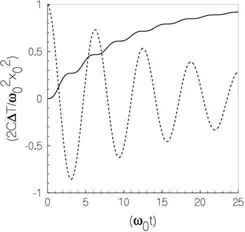
Figure 1: For an undamped oscillator with a quality factor $Q=\gamma/\omega_{0}=20.0$, plotted as a “dotted” curve is the relative displacement $x/x_{0}$ as a function of time. Plotted as a solid curve is the temperature change $\Delta T/(T_{\infty}-T_{0})$ wherein $T_{\infty}$ is the final equilibrium temperature after the oscillator stops moving.

If the harmonic oscillator has a constant specific heat $C$,

$$mC=T\frac{dS}{dT}\ ,$$ (34)

then Eqs.(31), (33) and (34) allow one to compute how the temperature of the oscillator will vary in time; i.e.

$$T(t)=T_{0}+\left(\frac{2\gamma}{C}\right)\int_{0}^{t}\dot{x}(t^{\prime})^{2}dt^{\prime}.$$ (35)

For the case of zero initial phase $\phi=0$,

$$\lim_{t\to\infty}T(t)\equiv T_{0}+T_{\infty}=T_{0}+\frac{m}{2}\omega_{0}^{2}x_{0}^{2},$$ (36)

one finds that the temperature increase $\Delta T=T-T_{0}$ obeys

$$\frac{2C\Delta T(t)}{\omega_{0}^{2}x_{0}^{2}}=1-e^{-2\omega_{0}t/Q}\times\ \ \ \ \ \ \ \ \ \ \$$

$$\left[1+\frac{\cos(2\Omega t)-1}{Q^{4}}+\left(1-\frac{1}{Q^{2}}\right)^{3/2}\frac{\sin(2\Omega t)}{Q}\right],$$ (37)

where the oscillation quality factor $Q=(\omega_{0}/\gamma)$. We have plotted both the damped harmonic oscillator coordinate and the the temperature increase $\Delta T$ in Fig.1 above as an illustration of how thermodynamic parameters as functions of time can be calculated similarly to computations of ordinary mechanical coordinates.

VI Conclusion

The classical formalism of mechanics was extended to also include consideration of entropy. The results allowed for a revised form of Lagrange’s and Hamilton’s equations which necessarily included energy dissipation due to frictional forces. It was shown that when the frictional forces vanished, that the entropy production was also $0$ and classical results were reproduced. However, in the diabatic cases, the law of energy conservation gave rise to the conventional condition of entropy production in both the Lagrangian and Hamiltonian frameworks. A simple example was then considered and worked out in detail where the rate of entropy production was connection to the heating rate. The explicit connection between the motion of a body and the rise in temperature was shown in closed analytical form. A more complicated problem such as the entry into the atmosphere and burn of a meteorite can in principle be treated by the methods here discussed although analytical solutions would appear unlikely.

References

- (1) L.D. Landau and E.M. Lifshitz, “Quantum Mechanics (Non-relativistic Theory),” Chap. 1-2, Butterworth Heinemann, Oxford (2003).
- (2) L.D. Landau and E.M. Lifshitz, “Statistical Physics,” Chap. 2, Butterworth Heinemann, Oxford (2001).
- (3) E. Fermi, “Thermodynamics,” Dover Publications Inc., (1956).
- (4) A.J. McMillan, “A non-linear model for self-excited vibrations,” Journal of Sound and Vibration 205, 323-335 (1997).
- (5) M.V. Drexel, J.H. Ginsberg, “Modal overlap and dissipation effects of a cantilever beam with multiple attached oscillators,” Journal of Vibration and Acoustics 123, 181-188 (2001).
- (6) R.W.S. Rayleigh, “The Theory of Sound: Volume 2,” Chap. 16, Dover Publications Inc, New York (1945).
- (7) L.D. Landau and E.M. Lifshitz, “Mechanics,” Chap. 1-2, 7, Butterworth Heinemann Oxford (2001).
- (8) F. Morabito et al., “Nonlinear antiwindup applied to euler lagrange systems,” IEEE Transactions on Robotics and Automation, 20, 526-537 (2004).
- (9) M. Razavy “Classical and Quantum Dissipative Systems,” Imperial College Press, London (2005).