On the Separability of Attractors in Grandmother Dynamic Systems with Structured Connectivity

Abstract

The combination of complex networks and dynamic systems research is poised to yield some of the most interesting theoretic and applied scientific results along the forthcoming decades. The present work addresses a particularly important related aspect, namely the quantification of how well separated can the attractors be in dynamic systems underlined by four types of complex networks (Erdős-Rényi, Barabási-Albert, Watts-Strogatz and as well as a geographic model). Attention is focused on grandmother dynamic systems, where each state variable (associated to each node) is used to represent a specific prototype pattern (attractor). By assuming that the attractors spread their influence among its neighboring nodes through a diffusive process, it is possible to overlook the specific details of specific dynamics and focus attention on the separability among such attractors. This property is defined in terms of two separation indices (one individual to each prototype and the other considering also the immediate neighborhood) reflecting the balance and proximity to attractors revealed by the activation of the network after a diffusive process. The separation index considering also the neighborhood was found to be much more informative, while the best separability was observed for the Watts-Strogatz and the geographic models. The effects of the involved parameters on the separability were investigated by correlation and path analyses. The obtained results suggest the special importance of some measurements in underlying the relationship between topology and dynamics.

‘Nothing in excess.’ (Delphic proverb)

I Introduction

Most dynamic systems, from neuronal networks to pattern formation, involves several interconnected variables, which can be properly represented in terms of a graph (e.g. West (2001); Bollobás (1990)) or complex network (e.g. Albert and A.-L.Barabási (2002); Dorogovtsev and Mendes (2002); Watts (2003); Wasserman and Faust (1994); Newman (2003); Boccaletti et al. (2006); da F. Costa et al. ). Such systems are henceforth called complex dynamic systems. A state variable $v(i)$ is normally associated to each node $i$, so that the complete evolution of the system can be described by the $N\times 1$ vector $\vec{v}^{(t)}$. In a neuronal network, for instance, each neuron can be expressed as a vertex (or a node), while synapses are represented by links (or edges) and the node activation by the respective state variable. Once the underlying connectivity of such a system is represented in terms of its weight matrix $W$ , several important types of dynamics can be subsumed as

$$\vec{v}^{(t+1)}=f(W\vec{v}^{(t)}).$$ (1)

Any layer of the perceptron neuronal network (e.g.  Rosenblatt (1958); Haykin (1999)), for instance, is obtained by substituting $f()$ by some abrupt function (e.g. hard limit or sigmoid). At the same time, the complete classic Hopfield model (e.g. Hopfield (1984); Haykin (1999)) can be represented by this equation. A simpler, linear model is obtained by making $f(x)=x$, so that $\vec{v}^{(t+1)}=W\vec{v}^{(t)}$. In case $W$ is also a stochastic matrix (the transition matrix), this linear equation subsumes all first order Markov chains, a particularly useful and important dynamic model which is intrinsically associated to random walks (e.g. Rudnik and Gaspari (2004)), Markov chains (e.g. Brémaud (2001)) and diffusion (e.g. Crank (1980); Havlin (2000)).

In many dynamic systems (e.g. Haykin (1999); Boccara (2004)), the codification of external stimuli as well as the results from the network dynamics take place in the $N-$dimensional space defined by the state variables. For instance, one particularly pattern may be represented as the state $\vec{v_{1}}=[1,0,-1,0.5,1,0]$, while another pattern may be associated to $\vec{v_{2}}=[0,1,-1,0,1,0]$. This type of representation is called  vector coding (e.g. Georgopouls et al. (1986); Salinas and Abbott (1994)). States which are near any of such pattern-states are frequently understood to be associated to that pattern. For instance, in the case of the example above, a third pattern similar to $\vec{v_{1}}$ will tend to be coded as a state vector $\vec{v_{3}}$ such that $\delta=||\vec{v_{1}}-\vec{v_{3}}||$ is small. Such a smooth, graded coding along the state space is interesting because it allows for some robustness/redundancy and flexibility/generality for the representation of the patterns, while also favoring good dynamic properties such as where the patterns are accessed through gradient-descent or similar methods (e.g. Haykin (1999); Rudnik and Gaspari (2004)).

However, it is also possible and interesting to consider the situation where the patterns are associated to specific nodes, not to specific points in the state space, such as in systems involving the so-called grandmother cells (e.g. Barlow (1972); Gross (2002); Gazzaniga et al. (1998)). Extremely important systems including great part of the mammals cortex are believed to be so organized. In these cases, a pattern is associated to a node $i$ such that high values of $v(i)$ signalizes the presence of that pattern. This type of cells is ubiquitous in several cortical areas (e.g. McIlwain (1996); Zeki (1990, 1999)). For instance, cells which are highly specific to hands and faces have been found in the inferior temporal cortex Gross et al. (1969); Perrett et al. (1982); Gross (2002). It is also known (e.g. Eichenbaum et al. (1989); McIlwain (1996); Zeki (1999); Bosking et al. (2002)) that much of the mammals cortical architecture is characterized by spatial smoothness, in the sense that cells which are spatially close tend to exhibit similar dynamics and response (i.e. state correlations), except at eventual singularities involving fractures Zeki (1999); Bosking et al. (2002). Such an organization reminds of the smooth coding discussed above for dynamic systems where patterns are represented by the overal state (i.e. vector coding). It is important to note that the smoothness property is not exclusive to topographically organized systems  such as the mammals cortex. In other words, even in networks where the nodes have no specific position in an embedding space, neighboring grandmother nodes may tend to have similar dynamics and response. In such cases, it is interesting to use the concept of progressive neighborhoods around a node (e.g. Faloutsos et al. (1999); Newman (2001); Cohen et al. (2003); da F. Costa (2004a); da F. Costa and da Silva (2006); da F. Costa and Silva (2007))), defined by the immediate neighbors of a node as well as its second neighbors, and so on. Following da F. Costa (2004a); da F. Costa and Silva (2007, 2007), in this work we organize the successive neighborhoods in terms of their hierarchical level. Therefore, the immediate neighbors of a node $i$ are at hierarchy 1 of $i$, and so on. In brief, the coding smoothness property in grandmother systems is reflected by the fact that the hierarchical neighbors of each node will tend to have responses similar, though progressively diverging, to that of node $i$.

In dynamic networks with a finite number of nodes, the situation considered herein, a particularly interesting problem arises as a consequence of a tension between the grandmother coding and the smoothness property, a phenomenon directly related to the limited number of patterns which can be properly represented (e.g. Amit and Brunel (1993)). Before proceeding further, it is important to provide a more objective characterization of such a problem. Consider that $M$ prototypic, distinct, patterns are to be represented in the network. If each of such patterns is represented by a respective prototypic neuron (node), in the sense that this neuron will be the most highly activate when that pattern is invoked by the network, we also need to allow for intermediate cells with graded replies between pairs of nodes. Observe that such prototype nodes typically act as attractors for the dynamics of the respective dynamic system, being accessed, for instance, by using gradient descent and/or random walks methods. If $M$ is too large, a point will be reached where each network node will be required to represent each prototypical pattern, running out of nodes for implementing the graded responses. Although this situation occurs at the very limit of the network capacity, it is important to observe that it may still provide a complete, invertible representation of the patterns (i.e. an one-to-one mapping). On the other hand, the smoothness of the coding is undermined as the number of prototypical patterns increases. In addition to destroying the network potential for generality and robustness, it will also become impossible to retrieve the patterns by gradient-descent like mechanisms along the network. Figure 1 illustrates two small topographic state spaces: one (a) corresponding to the limit situation where each pattern is associated to each node, the other (b) depicting a smooth map defined by diffusion around five prototype nodes. These two spaces were assumed to have local connectivity, in the sense that each cell communicates only with its most immediate neighbors in the orthogonal lattice. Observe that it is virtually impossible to devise an effective retrieval or activation mechanism capable of getting to any specific prototype node in Figure 1(a). In addition, the failure of any cell will imply in the irrecoverable lost of one pattern (the origin of the gradmother cell concept). On the other hand, the state space in Figure 1(b) allows a good level of tolerance to failure (this also means some redundancy), at the same time as simple dynamic mechanisms such as gradient descent can be employed for retrieving and activating nodes.

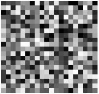
(a)

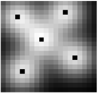
(b)

Figure 1: Gray-level visualizations of a topographic state space with too many prototypical patterns (a) and of a smooth topographic state space (b). Both these spaces are underlined by 4-neighborhood in the orthogonal lattice. The five prototype patterns in (b) have been marked in black for the sake of better visualization. 

For all that has been said above, it becomes very important to quantify and study the pattern separability in dynamic systems such as neuronal networks. In the case of the dynamic systems which can be fully represented by Equation 1, these two properties are necessarily implied by the network connectivity, defined by the weight matrix $W$, and the function $f()$. The present work focuses precisely on the investigation of the separability between patterns in grandmother complex dynamic systems. By considering a diffusive process emanating from each prototype node, followed by a process which assigns to each edge the difference between the activation states at its head and tail nodes, a graded representation of the prototype patterns can be obtained. This allows full generality of the reported investigations as an approximation to many types of grandmother dynamic systems. The accessibility to the original prototypes is simulated through a preferential random walk (diffusion) starting at every node of the network. After a given relaxation time, the activation of the network is normalized so as to correspond to occupancy probabilities and compared to the original prototypes position. This is done by considering two separation indices, one individual, considering the resulting activity only at the prototype nodes, and the other considering the activation not only at these nodes, but also at their immediate neighbors. These two indices, are henceforth abbreviated as $s_{ind}$ and $s$, are obtained in terms of the normalized geometric average of the activations at (or around) each prototype node. Therefore, the maximum value of these indices (equal to one) is achieved only when the resulting activation is totally and uniformly distributed among only the prototype nodes (for $s_{ind}$) or among these nodes and their immediate neighbros (for $s$).

The performed simulations and analyses first consider specific network configurations, in order to gather insights about the influence of each involved parameter, which are identified and discussed. Subsequently, a more systematic investigation of some parameter variations are performed. In order to infer the influence of the topologic features on the dynamics properties (i.e. attractors separation), we apply correlation analysis and path analysis. A series of interesting results are obtained regarding not only the separation indices, but also the importance of several local and global topologic features on the overall attractors separation. Although the current work concentrates on attractors in grandmother dynamic systems, several of the results, measurements and methods can be immediately extended to other relevant systems based on complex networks, including those involving information transfer and retrieval.

This article starts by presenting a brief review of more closely related works, and follows by describing the adopted notation and methodologies. Next, each of the four considered theoretic network models are briefly reviewed and their generation described. The diffusion procedure and ‘differentiation’ of the state values adopted to implement the attraction basins are described next, as well as the diffusion-base mechanism for activation/retrieval of prototypes. The two separation indices are motivated and mathematically defined. The simulation results and respective discussion are then presented, followed by the correlation and path analyses of the effects of the topologic features of the network on the respective attractors separability. Several interesting findings and effects are identified and discussed. The article concludes with a general synthesis of the reported investigation and with identification of possible future developments.

II A Brief Review of Previous Developments

The subject of attractor characterization has been extensively addressed in the literature, so we limit ourselves to reviewing a small subset of those works which are more general or more directly related to the investigations being considered in the present work.

A comprehensive study of attractor networks has been presented by Amit Amit (1992). Torres et al. have considered the storage capacity of attractor neural networks in which the synapses can undergo depression Torres et al. (2002) and found that the memory capacity decreases with the intensity of the depression. Amit and Brunel Amit and Brunel (1993) investigated learning in attractor networks considering the effects of stimuli in a network with wired-up patterns. Topographic neuronal networks involving grandmother cells have been extensively studied by T. Kohonen and collaborators (e.g. Kohonen (1982); Oja et al. (2003); Kohonen (2006)) in the form of the self-organizing map (SOM) or Kohonen networks. Here, the neurons are spatially distributed and develop specificity to prototype pattern stimuli by influencing the weights of neighboring nodes. Therefore, spatially adjacent smooth attraction basins are defined.

Several works have brought together the two important areas of complex networks and dynamic systems, including neuronal networks. At least two excellent surveys have been written about this important issue Newman (2003); Boccaletti et al. (2006). The problem of neuronal structure and dynamics has also been a subject of growing interest, including but by no means limited to da F. Costa (2005a); Peichl and Waessle (1983); da F. Costa et al. (2003); da F. Costa (2003a); Samsonovich and Ascoli (2005); van Ooyen et al. (1995); Ooyen and Willshaw (1999); Ooyen et al. (2001); Graham and Ooyen (2004). Stauffer et al. Stauffer et al. (2003) investigated the performance of diluted Hopfield networks underlined by the BA model. The influence of the network topology on the dynamics of neural networks has been investigated also by Costa and Stauffer da F. Costa and Stauffer (2003), who considered spatial neural networks and concluded that its performance increased with the spatial uniformity of the cells distribution. Torres et al. Torres et al. (2004), showed that the pattern capacity of an attractor neural network with scale free topology is higher than for a random-diluted network with the same number of connections. They also found that, at zero temperature, the performance of scale free nets improves for larger values of the power-law exponent. Models of non-randomly diluted neuronal networks whose connectivity is determined as a function of the shape of its individual neurons (as well as their relative spatial positions) has been reported by Costa and collaborators da F. Costa et al. (2003); da F. Costa and Barbosa (2004). It was found that the shape of individual neurons can have a great influence on the respective memory capacity, suggesting that shapes more similar to real neurons tend to have better attractor properties. The influence of the network topology on the recovery of patterns in recurrent neuronal networks was addressed by Castillo et al. Castillo et al. (2004). Their work showed that the retrieval properties can be enhanced by considering connectivity more structured than in random networks. Morelli et al. Morelli et al. (2004) investigated the memory capacity in associative networks and found that the best performance is obtained at an intermediate level of disorder. Zhou and Lipowski Zhou and Lipowski (2005) investigated, through analytic and simulation means, a general class of dynamic systems on scale free networks with binary states. They reported important variations of performance with respect to the scale free exponential coefficient. The effect of structured connections on the interactive statistical mechanics algorithm for minimization of the Bethe free energy (associated to Ising models) has been studied by Ohkubo et al. Ohkubo et al. (2005). The adaptation of the Sznajd dynamics to take place over the network connectivity instead of its states has been reported by Costa da F. Costa (2005b), yielding network realizations which are a consequence of an inherent dynamical process. Lu et al. Lu et al. (2006) considered the effect of regular, random, small-world and scale free topologies on Hopfield networks. They reported, among other findings, that the performance improved with the local order of the connections, which seems to be in agreement with da F. Costa and Stauffer (2003). The periodicity of activity in networks with small-world and scale-free topologies were investigated by Paula et al. Paula et al. (2006) who concluded, among other findings, that periodic activity appears only for relatively small networks. Perotti et al. Perotti et al. (2006) studied the interesting problem of associative memory on a growing diluted Hopfield model which converges to a small-world, scale free topology and showed that the performance of such a network is higher than that of a randomly diluted network with the same connectivity. More recently, Davey et al. Davey et al. (2006) investigated sparse small world associative memory considering Perceptron training under small world connectivity ranging from local to global and found that non-symmetric connectivity networks exhibited superior performance. By considering random walks as a reference model for implementing dynamics in complex networks, Costa et al. investigated the correlations between the topology (node degree) and activation (frequency of visits to nodes at equilibrium). They found that while full correlation is guaranteed for undirected networks, it can vary substantially in directed networks such as biological neuronal networks and the Internet, implying that topologic hubs are not necessarily hubs of activity. That work also identified a relationship between scale free networks and the Zipf’s law Newman (2005). A study of self-organizing models underlined by complex networks related to mental processes has been reported by Wedemann et al. Wedemann et al. (2006). The investigation of the relationship between topology and dynamics at higher spatial scales (e.g. cortical areas) has also been addressed in an increasing number of works (e.g. Sporns (2002); Hilgetag et al. (2002, 2000); Sporns et al. (2000a, b); da F. Costa and Sporns (2006, 2007); da F. Costa et al. (2006)).

Increasing attention has also been drawn on the synchronization of oscillations as the means for pattern encoding and retrieval (e.g. Arecchi (2004)). Among the works related to the separation of attractors, Arecchi Arecchi (2005) has considered a metric structure for the percept space, while taking into account the separation between states. Wang et al. investigated the influence of the node degree distribution in the synchronization of two-layer neural networks. The criticality of coupling parameters on the synchronization of an ensemble of identical neural networks with small-world topology has been addressed by Wang et al. Wang et al. (2005).

All in all, as far as the influence of connectivity on the performance of dynamic systems for storing patterns is concerned, several of the above reviewed works seem to indicate that better results tend to be obtained by considering non-random connectivity, but at a level of order that ranges from low to intermediate.

III Notation, Basic Concepts and Methodology

This section covers the concepts and methods used in the current investigation. Its subsections present the basic concepts and measurements in complex networks, the four considered theoretic network models, the procedure suggested to extend the prototype influence through their successive neighborhoods in order to establish the attraction basins, the diffusive way to activate the attractors, the separation measurements, and the correlation and path analyses considered in this work.

III.1 Complex Networks Concepts and Topologic Measurements

A graph $\Gamma$ involves a set $V$ of $N$ nodes interconnected by a set $U$ of $E$ edges, i.e. $\Gamma=(V,U)$. Each directed edge linking a node $i$ to a node $j$ is represented as $(i,j)$. Such a graph can be conveniently expressed in terms of its adjacency matrix $K$, so that $K(j,i)=1$ whenever an edge $(i,j)$ exists (otherwise, $K(j,i)=0$). A graph such that $K(i,j)=K(j,i)=1$ is said to be non-oriented. Although the present work focuses on this type of graph, all reported developments can be extended to directed graphs. The graphs considered henceforth are also devoid of self-connections (i.e. $K(i,i)=0$ for every node $i$). A complex network is henceforth understood as a graph exhibiting a particularly intricated structure, in the sense of differing from a random graph of the Erdős-Rényi type Erdős and Rényi (1959, 1960). However, because of statistic fluctuations, a random graph can also exhibit intricated structure.

Given a generic node $i$, some measurements can be associated to it (e.g. Albert and A.-L.Barabási (2002); Newman (2003); da F. Costa et al. ). Its degree $k(i)$ is defined as the number of edges attached to it, so that

$$k(i)=\sum_{p=1}^{N}K(p,i).$$ (2)

The immediate neighbors of a node $i$ correspond to those nodes which are directly attached to it. The clustering coefficient of a node $i$ expresses the degree of connectivity among its immediate neighbors and can be calculated as

$$cc(i)=\frac{e(i)}{e_{max}},$$ (3)

where $e(i)$ is the number of undirected edges between the immediate neighbors of $i$ and $e_{max}$ is the maximum possible number of such connections, given as $e_{max}=e(i)(e(i)-1)/2$.

The shortest path between any two nodes $i$ and $j$ corresponds to the minimal set $SP$ of adjacent edges connecting those two nodes. A network in which all nodes can be reached, through paths, from any other node is henceforth said to be connected. The respective shortest path length $sp$ is defined as the number of edges in $SP$. Therefore, the immediate neighbors of a node $i$ can be alternatively defined as the nodes which are at shortest path length of 1 from node $i$. The second neighborhood (or neighbors of second hierarchy) are those nodes which are at shortest path length of 2 from $i$, and so on. The maximum shortest path length between any pair of nodes is defined as the network diameter, henceforth abbreviated as $diam$.

Given a set $R$ of $M$ reference (or seed) nodes, it is possible to obtain the respective Voronoi tessellation Stoyan et al. (1996) of the network da F. Costa and Silva (2007) with respect to the seeds, which partitions the $N$ nodes into $M$ connected subgraphs associated to each of the reference nodes. This can be achieved by, for each node $i$, identifying which of the reference nodes is closest (in the sense of shortest path) to $i$ and assigning it to that region. Given two nodes $i$ and $j$, whose respective immediate neighbors are represented by the sets $n(i)$ and $n(j)$, we define their common neighbors as the set $c(i)=n(i)\cap n(j)$. Given the Voronoi partition of a network, it is interesting to devise a measurement capable of expressing the uniformity of the areas $A(i)$ (i.e. number of nodes) of each of the $M$ partitioned regions $i$. This can be conveniently achieved by considering the geometric average $\left[A\right]$ of the areas, i.e.

$$\left[A\right]=\left(\prod_{i=1}^{M}A(i)\right)^{1/M},$$ (4)

Observe that the geometric average implies a high penalty on higher variations of the Voronoi areas, therefore providing a more strict quantification of the homogeneity of those areas. Figure 2 illustrates the comparison between the arithmetic and geometric average considering two measurements $p$ (with $0\leq p\leq 1$) and $q=1-p$. The ability of the geometric average in quantifying the similarity between $p$ and $q$ is evident from this figure. While dispersion-related measurements (e.g. standard deviation and entropy of the state activations) could be used, they could not be interepreted as quantifications of the activations.

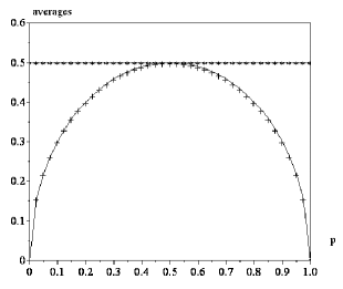
Figure 2: The arithmetic ($*$) and geometric ($+$) averages between the values $p$ and $q=1-p$. The geometric average allows the quantification of the uniformity between the values of $p$ and $q$, with a peak at $p=q=0.5$. 

As the geometric average $u$ for the $M$ Voronoi areas varies as $0\leq u\leq 1/M$, it is convenient to redefined $\left[A\right]$ as

$$\left[A\right]=M\left(\prod_{i=1}^{P}A(i)\right)^{1/M}.$$ (5)

The matching index Sporns (2002); Hilgetag et al. (2002) of a pair of nodes $i$ and $j$, expressing the relative degree of overlap between the immediate neighborhoods of those nodes, can be calculated as

$$mi(i,j)=\frac{n(i)\cap n(j)}{n(i)\cup n(j)}.$$ (6)

This measurement gives the fraction of immediate neighbors of $i$ and $j$ which are common neighbors to them both. For instance, for the situation depicted in Figure 4, we have that the matching index of the pair of nodes $P1$ and $P2$ is given as $m(P1,P2)=2/8=0.25$.

III.2 Complex Networks Theoretic Models

Four theoretic models of complex networks are considered in the present work: Erdős-Rényi (ER), Barabási-Albert (BA), Watts-Strogatz (WS) and a geographic model (GG). Reflecting their different natures and organizing principles, these models correspond to a significant portion of the complex networks found in nature, providing therefore a representative choice of models for the current study of attractor separability. In order to account for a more coherent comparison between the separability of attractors in these four models, each comparison always consider $N$ and $\left<k\right>$ for each model to be as similar as possible . In this work, the average degree of the BA model (defined by the parameter $m$) is always taken as a reference for defining the average degree of the other models. The methodology for constructing such models are described in the following subsections.

III.2.1 Erdős-Rényi

Random networks, also called Erdős-Rényi – ER, were among the first models of stochastic networks to be extensively studied(e.g. Rapoport (1957); Erdős and Rényi (1959, 1960)). These networks are characterized by constant probability of having a connection between any of the possible pairs of nodes, and are therefore related to Poisson processes. The connectivity of ER networks can generally be well approximated in terms of its average degree, implying that such networks are similar to regular networks, characterized by having the same degree at any of its nodes. As a consequence of its indiscriminate connectivity and largely regular organization, the ER type of networks does not typically provide a good model of natural structures and phenomena, where the connections tend to follow more purposive and specific rules.

In an ER graph, each possible connection between each possible pair of nodes, has constant probability $\gamma$ of existence. Such networks can be easily created through Monte Carlo simulation by making $K(i,j)=K(j,i)=1$, with $i\neq j$, with probability $\gamma$. Observe that the construction of ER networks consider only two parameters: $N$ and $\gamma$. In order to obtain values of $\left<k\right>$ similar to the BA reference, we enforce $\gamma=2m/(N-1)$, where $m$ is a parameter of the BA model (see next subsection).

III.2.2 Barabási-Albert

The so-called Barabási-Albert model Albert et al. (1999); Barabási (2002); Albert and A.-L.Barabási (2002) – BA, belongs to the important class of scale free networks. This type of network is characterized by the fact that the loglog plot of their node degrees tends to a straight line, implying the absence of any characteristic scale. In other words, the node distribution in such a network follows a power law. One of the most important properties of scale free networks (e.g. Albert and A.-L.Barabási (2002); Barabási (2002)), when compared to models such as the ER, is the higher probability of existence of hubs, i.e. nodes with particularly high degree. Such special nodes are particularly important in defining the connectivity and topologic features of the network, such as the average shortest path length. For instance, the fact that a hub connects to many nodes immediately implies that the shortest path between any of these nodes will be at most equal to 2 edges. Several important natural and human-made structures – including the Internet, WWW, protein interaction and even scientific collaborations – have been found to exhibit the scale free property (e.g. Albert and A.-L.Barabási (2002); Barabási (2002); Newman (2003)). The BA model incorporates the so-called rich-get-richer paradigm because of its attachment of links being preferential to the degree of existing nodes.

In the current work, BA networks are generated starting with $m0$ randomly connected nodes. At each subsequent step, a new node with $m$ edges is added to the network, with each of the $m$ edges being attached to previous network nodes preferentially to their degree. Therefore, each new connection is more likely to be established with previous nodes with high degree, implementing the ‘rich get richer’ paradigm. As with the ER model, the construction of BA networks also involves only two parameters: $N$ and $m$.

III.2.3 Watts-Strogatz

Historically, the small world networks of Watts and Strogatz Watts and Strogatz (1998); Watts (2003) followed the random networks of Erdős, Rényi and collaborators. Small world networks are exactly as implied by their name, i.e. the average shortest path length between their nodes tends to be small. At the same time, they also tend to be characterized by relatively high clustering coefficient, implying that they local connectivity is relatively high. The small world property, which has been found to be present in many interesting networks including ER and BA, has important implications for the separation of attractors because it implies that many prototype nodes will be near one another and, consequently, possibly less separated as far as the dynamics is concerned. The WS model considered in this work, however, presents some specific topologic organization which has potential implications for the distribution of the prototypes. More specifically, this model is characterized by a relatively high regularity and uniformity of local connectivity.

The Watts-Strogatz networks used in the current work have been constructed by starting with a ring of nodes where each node is connected to its $m$ clockwise and anti-clockwise nodes. After such an initial network is obtained, $\alpha$% of the existing connections are rewired at random. This network model involves three parameters: $N$, $m$ and $\alpha$. All configurations in this work assume $\alpha=10$%.

III.2.4 A Geographic Model

Geographic networks (e.g.da F. Costa and Stauffer (2003); da F. Costa (2003b); Pastor-Satorras and Vespignani (2004); da F. Costa and Diambra (2005); Barrat et al. (2005); Gastner and Newman (2006))) – also called spatial, geometric or topologic – are characterized by the fact that their nodes have well-defined spatial positions within an embedding space. Frequently, the connectivity in such networks is considered to be highly influenced by the spatial adjacencies and/or spatial proximity between its nodes, in the sense that two nodes which are adjacent or near one another will have higher chances of being connected. Therefore, geographic models in small dimensional spaces (e.g. 2D or 3D) tend not to be small world. Such a property is particularly important as far as the separation of the prototype nodes is concerned because, in principle, this type of network allows more space distribution of nodes which are relatively further apart. Here, we consider one of the simplest possible approaches to obtaining a geographic model, which involves the distribution of the $N$ nodes uniformly along a 2D space followed by the interconnection of all nodes which are closer than a given distance $d$.

In order to build a GG network, we start with an empty $L\times L$ discrete space $S$, such that each of its positions is expressed as $S(x,y)$, where $i$ and $j$ are integer values so that $1\leq x,y\leq N$. This space is henceforth understood as a Poisson field with density $\rho$, in the sense that any region with area $a$ (i.e. number of discrete elements $(x,y)$) will have, in the average, a total of $a\rho$ points marked as $S(x,y)=1$ Stoyan et al. (1996). The network nodes are selected by considering each position $(x,y)$ in the space $S$ with probability $\rho=N/L^{2}$, implying an average total number of nodes $N$. Then, each of such nodes, marked as $S(x,y)=1$, is connected to all other nodes to be found up to a maximum Euclidean distance $d$. Therefore, the average degree of the network can be defined by controlling $d$. More specifically, we make $d=L\sqrt{2m/(N\pi)}$, so that every disk of radius $r$ in $S$ centered at each node will contain, in the average, $\left<k\right>=2m$, where $m$ is the BA parameter taken as the reference. The growth parameters of such a network model therefore are again limited to only $N$ and $m$. In order to ensure a relatively small variation of $N$, every generated network with a total number of nodes smaller than 90% of the desired value of $N$ were discarded. Figure 3 illustrates a GG complex network obtained by using the methodology described above for $N=50$ and $m=3$.

III.3 Generating the Attraction Basins

As indicated in the Introduction, in order to avoid the intricacies and specificities of how each distinct dynamic system represents attractors, here we resort to a simple methodology involving diffusion of activity from the prototype nodes, followed by the transformation of the so obtained activity into a derivative network da F. Costa (2004b); da F. Costa and Travieso (2005). Although not reproducing in detail the attraction basins which would be otherwise produced by diverse specific dynamics, this approach does ensure the smoothness of coding, i.e. the property that nodes which are topologic close will tend to have similar state dynamics. The details of such a methodology are presented as follows.

Let the $M$ prototype patterns be associated with respective nodes chosen with uniform probability among the $N$ network nodes. Let $\vec{P}$ be the vector such that $P(i)=1$ if and only $i$ is one of the prototype nodes, with $P(i)=0$ otherwise. In order to allow a probabilistic interpretation, we normalize this vector as $\vec{p}=\vec{P}/\sum_{i=1}^{N}p(i)$. This vector will act as the fixed source of probabilities during the diffusion. The adjacency matrix describing the network is also normalized into its respective transfer matrix $W$, i.e.:

$$W(i,j)=K(i,j)/k(i),$$ (7)

where $k(i)$ is the degree of node $i$. Note that all the sums of $W$ along each of its columns will now be equal to 1, i.e. $W$ is a stochastic matrix. In order to ensure that the matrix $K$ is connected (irreducible) Brémaud (2001), all the nodes which do not belong to the main connected component are excluded from the network at the end of its respective construction. Because the considered average node degrees are relatively high, and well above the percolation critic density, very few nodes are removed through such a procedure.

Now, the final distribution of occupancy $\vec{\Omega^{T}}$ of each node $i$ after $T$ interactions can be calculated by applying recursively ($T$ times) the following set of equations:

$$\vec{a}=\left(\vec{\Omega}^{t}+\vec{p}\right),$$

$$\vec{b}=\left(\vec{a}/\sum_{i=1}^{N}a(i)\right),$$

$$\vec{\Omega}^{t+1}=W\vec{b}.$$ (8)

The number $T_{t}$ of total interactions is henceforth defined as corresponding to $3$ times the diameter of the respective network, i.e. $T_{t}=3diam$. Figure 3(b) illustrates the occupancy states obtained for a GG network with $N=100$, $\left<k\right>=6$ and $M=2$ after $T_{t}=27$ interactions.

After the occupancy state of each node is obtained for the network, its respective derivative network $\Delta$ (e.g. da F. Costa (2004b); da F. Costa and Travieso (2005)) is obtained by applying the equation below for each edge $(i,j)$ existing in the original network.

$$aux=\Omega(j)-\Omega(i)$$

$$\left\{\begin{array}[]{ll}aux>0\Rightarrow&\Delta(j,i)=aux\\ aux<0\Rightarrow&\Delta(j,i)=aux/10\\ aux=0\Rightarrow&\Delta(j,i)=-1\\ \end{array}\right.$$

The following substitution is applied afterwards:

$$\Delta(j,i)=-1\Rightarrow\Delta(j,i)=max(\Delta)/\beta.$$ (10)

All cases in this work assumes $\beta=1000$, but this parameters has been found not to be critical.

Note that the values $\Delta(j,i)$ correspond to the weights of the respective edges $(i,j)$. Those edges which connect a node with small induced activity to a node with higher activity will have larger weights. More specifically, in case $aux>0$ the weights are directly proportional to the difference of activations. Edges leading from higher to smaller activations have one tenth of the reciprocal edge. Because several adjacent nodes may result with equal activations, the eventual previous connectivity between then will be preserved though at an incremental value proportional to the maximum activation (Equation 10). Observe that the matrix $\Delta$ is not symmetric.

III.4 Activating the Network

Once the derivative network defined by the weight matrix $\Delta$ has been calculated, its activation can be easily achieved through a random walk preferential to the weights of the edges (see also Toroczkai and Bassler (2004), where information is transmitted considering the gradient of a node). In order to do so, we obtain the stochastic version of $\Delta$ by applying the following equation to each of its edge $(i,j)$

$$\delta(j,i)=\Delta(j,i)/\sum_{j=1}^{N}\Delta(j,i).$$ (11)

The activation after $T$ steps is now given as

$$\vec{\alpha}=1/N\delta^{T}\vec{1},$$ (12)

where $\vec{1}$ is the $N\times 1$ vector of ones. As before, we assume that the total number of interactions $T_{r}$ is equal to 3 times the network diameter. Therefore, the final activation corresponds to the near equilibrium occupancy of each node after starting from any node. Figure 3(c) shows the activations obtained by the method described above with respect to the network in Figure 3(b). It is interesting to note that the peaks of the obtained activations do not necessarily correspond to the original prototype nodes. This is an interesting consequence of the fact that the activation of the derivative network is affected not only by the attraction basins, but also by the in-strength  and the local connectivity of each node. More specifically da F. Costa et al. (2006), in case the in-strength is equal to the out-strength for all nodes, the equilibrium activation will be directly proportional to the respective in-strength. However, this result is not guaranteed for asymmetric connectivity such as in the derivative network.

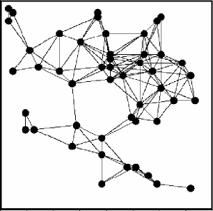
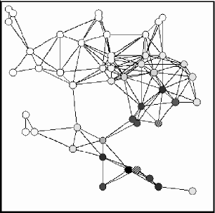
(a)                                                                       (b)

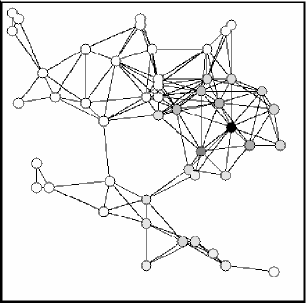
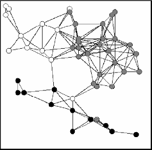
(c)                                                                       (d)

Figure 3: Example of GG network obtained for $N=50$ and $m=3$ (with $\left<k\right>=5.5$) (a). The respective occupancy states, defining the basis of the prototype nodes (striped), after $27$ interactions (b). Note the smooth distribution of states through both the topologic neighborhoods. The activation induced by the random walks preferential to the weights of the respective derivative network (c). The Voronoi tessellation defined by the two prototype nodes (represented as striped) (d). 

III.5 Separation Indices

Given a specific grandmother dynamic system, it is important to quantify in an objective manner the separability of its attractors. Recall that the system incorporates $M$ prototype patterns, associated to respective prototype nodes $p=1,2,\ldots,M$. In this work we propose two separation indices, $s_{ind}$ and $s_{ngh}$, defined by taking into account diffusion dynamics along the complex network underlying the dynamic system. For simplicity’s sake, the latter is henceforth called simply as separation index and abbreviated as $s$.

Once the activations have been obtained in each of the dynamic states associated to the nodes, we define the individual separation index $s_{ind}$ as being proportional to the geometric average of the activations $v(p)$ at each prototype node $p=1,2,\ldots,M$, i.e.

$$s_{ind}=M\left(\prod_{i=1}^{M}v(i)\right)^{1/M},$$ (13)

where the proportionality factor $M$ is introduced in order to ensure that $0\leq w\leq 1$ instead of $0\leq w\leq 1/M$. As with the quantification of the uniformity of the Voronoi areas (Section III.1), the geometric average will reach its maximum when all activations $v(i)$ have the same value.

However, as preliminary simulations (see Section IV.2) showed that this index tends to be too small, an alternative separation index has been considered which takes into account also the immediate neighborhoods of each prototype node. Consider the situation illustrated in Figure 4. This figure shows two prototype nodes $P1$ and $P2$ as well as their common $C$ immediate neighboring nodes. Because these nodes are at the same shortest path distance from $P1$ and $P2$, they do not contribute to the discrimination between those prototype nodes and are therefore not considered in the calculation of the neighborhood separation index, which is more formally defined as follows.

Let $Z(i)$ be the set including the respective prototype node $i$ and its immediated neighbors which are not common to the immediated neighborhoods of any of the other prototype nodes. The probability $p(i)$ at this set of nodes corresponds to the sum of the normalized activations of the states in $Z(i)$. Ideally, all prototype nodes should result with probability equal to $1/M$, implying that all prototypes are equally accessible and therefore maximally separable. In order to quantify how the obtained network state approaches such a reference separation, we define the neighborhood separation index $s_{ngh}$ as corresponding to the geometric average of the total probabilities at each set $Z(i)$, for all $M$ prototype nodes $i$, i.e.

$$s=s_{ngh}=M\left(\prod_{i=1}^{M}p(i)\right)^{1/M},$$ (14)

where the multiplying constant $M$ is, as before, included in order to imply that $0\leq s\leq 1$. The maximum separation between attractors is therefore obtained whenever $s=1$.

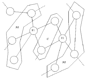
Figure 4: A portion of a hypothetical network showing two prototype nodes ($P1$ and $P2$). The nodes belonging to both immediate neighborhoods are identified by the region $C$, while the nodes belonging to the respective immediate neighborhoods minus the common nodes are enclosed by the regions $N1$ and $N2$, respectively. 

III.6 Correlation Analysis

Given several measurements of the topology of the network under analysis, as well as the separation indices, a first insight about their possible relationship and redundancy can be obtained by considering the Pearson correlation coefficient. Let us express each measurement as a random variable $X$ of which we have $N_{X}$ observations. First, we standardize Johnson and Wichern (2002) the variable $X$ as

$$\tilde{X}=\frac{X-\mu_{X}}{\sigma(X)},$$ (15)

where $\mu_{X}$ and $\sigma(X)$ are the estimate of the average and standard deviation of $X$. The new, normalized variable has average zero and unit variance. The Pearson correlation coefficient $r(X,Y)$ between any pair of normalized measurements $X$ and $Y$ can now be estimated as

$$r(X,Y)=\frac{1}{N_{X}-1}\sum_{i=1}^{N}\tilde{X}\tilde{Y}.$$ (16)

Observe that $-1\leq r(X,Y)\leq 1$, while $r(X,Y)=0$ means lack of correlation between the two measurements. It is important to stress that uncorrelation does not imply statistic independence. At the same time, correlation can by no means be understood as a certain indication of causality. In case two measurements result with high absolute value of the Pearson correlation coefficient, they are said to be correlated, indicating redundancy of measurements. However, even correlated measurements can contribute to the characterization and discrimination between the networks da F. Costa et al. .

III.7 Path Analysis

While the Pearson correlation coefficient quantifies, in a normalized fashion, the joint variation of two measurements, such a pairwise measurement does not consider information about additional measurements. A series of sound statistic methods, ranging from multivariate regression (e.g. Kleinbaum et al. (1998); Montgomery et al. (2001)) to the more sophisticated Structural Equation Modeling (SEM) (e.g. Raykov and Marcoulides (2000); Kline (2005)), can be considered in order to obtain a more representative characterization of the relationship between multiple random variables (including latent variables) or measurements. In this work we considered the Path Analysis methodology (e.g. Wright (1920); Raykov and Marcoulides (2000); Kline (2005)), understood here as a particular case of the SEM framework, in order to obtain indication about the influence of the several measurements of the topology of the networks on the respective attractor separation indices.

Path analysis was largely developed by S. Wright (e.g. Wright (1920)) in order to model explanatory relationships between observed variables. This methodology is similar to the solution of a system of equations implied by substituting the model generated covariance matrix into the sample covariance Raykov and Marcoulides (2000). One of the interesting features of this approach is that it considers the influence of the covariances between all variables, sometimes being closely related to multivariate linear regression. The path analysis performed in this work considers the structural relationship between the topologic and dynamic properties of the investigated networks as shown in Figure 5. A relatively simple relationship between the measurements has been considered, where the topologic features are understood to cause the dynamic properties, namely the individual and neighborhood attractor separation indices ($s_{ind}$ and $s$, respectively). Each of the measurements are associated to a reference number (upper righthand side of each box). The parameters $\gamma_{i}j$, which are in principle not known, express the importance of the topologic measurements with respect to the separation indices.

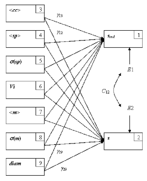
Figure 5: The structural relationship between the topologic and dynamic measurements considered for the path analysis reported in this work. The covariances between variables 3 to 9 are not shown for simplicity’s sake. 

Equations 17 and 18 express the relationship between the considered variables, reflecting the fact that the regression coefficients $\gamma_{i}j$ establish the weights of the influences of each topologic variable onto the two separation indices. The environment LISREL  was used in this work in order to perform path analysis.

$$s_{ind}\propto\gamma_{13}\left<cc\right>+\gamma_{14}\left<sp\right>+\gamma_{15}\sigma{sp}+\gamma_{16}Vi$$

$$+\gamma_{17}\left<mi\right>+\gamma_{18}\sigma(mi)+\gamma_{19}diam$$ (17)

$$s\propto\gamma_{13}\left<cc\right>+\gamma_{14}\left<sp\right>+\gamma_{15}\sigma{sp}+\gamma_{16}Vi$$

$$+\gamma_{17}\left<mi\right>+\gamma_{18}\sigma(mi)+\gamma_{19}diam$$ (18)

IV Results and Discussion

This section starts by identifying each involved parameter which can affect the simulations and follows by presenting the results obtained for specific configurations of $N$ and $m$ and an analysis of the variation of the parameters. The statistic analysis of the relationship between the topologic and dynamic measurements by using correlation and path analyses is also reported.

IV.1 Involved Parameters and Their Expected Effects

An important first issue to be considered while investigating the attractors separation in complex dynamic networks concerns the identification of all involved parameters which can influence the results. The parameters involved in our simulations, as well as their expected effects, are described in the following:

The network model and its intrinsic parameters: Each theoretic model of complex network considered in this work is likely to yield different attractors separations. Those networks characterized by the small world property (i.e. ER, BA and WS) are, in principle, likely to produce less separated attraction basis because of the relatively small shortest path distance, expected in the average, between the prototype nodes (however, see Section IV.5)). While the ER, BA and GG models can be generated by considering just two parameters (i.e. $N$ and $m$), the WS network also involves a third parameters corresponding to the percentage of rewirings, which is fixed as $\alpha=10$%.

The network size $N$: This is an important global parameter of every complex network, corresponding to its total number of nodes. One of the most important aspects related to this parameter are the so-called finite size effects, namely the fact that the network properties change considerably when moving from large (possibly infinite) to small values of $N$. As an extreme example, the connectivity of any network will decrease when $N$ approaches just one or two nodes. Although in this work we are more interested in finite size networks, it is often useful to try to extrapolate from properties measured for smaller values of $N$ to the infinite limit, as done in Section IV.3. Because of the computational demand required to simulate hundreds of realizations for each configuration, the current work is limited to relatively small values of $N$. As far as the attractors separation is concerned, it is expected that, for fixed $m$ and $M$, the separability will tend to increase with $N$ because of the additional space thus allowed for the representation and distribution of the prototypes.

The network average node degree $\left<k\right>$: This parameter, which in this work is defined with respect to the reference $m$, is particularly important in defining the overall degree of connectivity in the network, especially in those structures which are not scale free and therefore have specific degree scales. Generally, smaller values of $\left<k\right>$ tend to imply longer shortest paths, possibly improving the attractors separation (however, see Section IV.5). This parameter is not systematically investigated in this work, which mostly considers fixed $m=3$ (however, a situation with $m=10$ is considered in Section IV.2).

The number $M$ of prototype patterns to be represented: This parameter is directly involved in the separability of the prototype patterns, in the sense that the larger the number of prototypes, the less separated they tend to be.

The number $T_{t}$ of interactions used for diffusion around each prototype node: The diffusion of activity emanating from the prototype nodes has been verified to converge quickly for all considered networks, so that the assumption of the total number of interactions to be given as $T_{t}=3diam$ practically ensures the resulting activity to correspond to its equilibrium state.

The number $T_{r}$ of interactions considered in the retrieval random walk: Again, the assumed total number of interactions used in the activation of the attraction basins is large enough to imply near equilibrium states.

IV.2 Fixed Configurations

In order to get a better understanding about the separability of the attractors in the considered four theoretic models and to obtain preliminary indications about the effects of the involved parameters, we considered a set of preliminary simulations as described in the following. All results presented in this section considered $T_{t}=T_{r}=3diam$ and 500 realizations of each configuration.

So as to have the first glimpses of the separability in each of the four complex networks models, we considered $N=100$, $\left<k\right>=3$, and a relatively small number of prototypes $M=3$. The individual separation indices $s_{ind}$ and $s$ obtained for each of the four models are shown in terms of their respective population histograms in Figures 6 and 7. The respective averages and standard deviations are also shown inside each graph. The first important result is that the individual separation index $s_{ind}$ allows considerably less resolution than the neighborhood index $s$, with most of its values being close to zero (Fig. 6). As this effect has been confirmed for other configurations, we henceforth focus attention on the neighborhood separation index $s$. Interestingly, similar distributions have been obtained for the pairs of models ER/BA and WS/GG in Figure 7, the former being characterized by smaller averages of $s$. Observe also the presence of cases where $s=0$ in the WS and GG cases. The largest average, implying the better average attractor separability, was obtained for the WS model, followed by the GG networks, which also implied a significant number of null separability indices. This phenomenon is caused whenever all immediate neighbors of the prototype nodes are common. These results also show that a reasonable separation between the three prototype attractors have been obtained for the WS and GG cases.

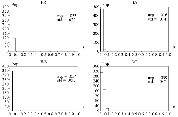
Figure 6: The population histograms of the separation index $s_{ind}$ for the four considered theoretic models of complex networks with $N=100$, $M=3$ and $\left<k\right>=6$ (i.e. $m=3$). It is clear from these histograms that the separation index $s_{ind}$ does not provide good resolution. 

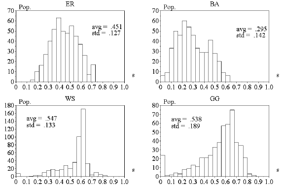
Figure 7: The population histograms of the separation index $s$ for the four considered theoretic models of complex networks with $N=100$, $M=3$ and $\left<k\right>=6$. Similar results were obtained for the ER/BA and WS/GG models. The former case involves smaller average and standard deviation of the $s$ index. 

Next, we verify the possible influence of the network size $N$ by considering the same configuration as before, but with $N=200$. The respective results are shown in Figure 8. It is clear from these results that the larger size of the network had relatively little influence on the separation indices, suggesting the finite size effect to be small for this number of parameters.

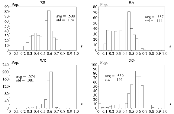
Figure 8: The population histograms of the separation index $s$ for the four considered theoretic models of complex networks with $N=200$, $M=3$ and $\left<k\right>=6$. Similar results were obtained for the ER/BA and WS/GG models. The results are similar to those obtained for $N=100$ (see Figure 7). 

Now we turn our attention to the influence of the number of prototype patterns to be represented. The same configuration as in Figure 7 is considered, except that $M=10$. The obtained results are shown in Figure 9. It is clear that increase by more than threefold of the number of prototype patterns implied not only a substantially more cases such that $s=0$, but also the distributions to be strongly left-shifted in comparison with the respective cases in Figure 7. This effect holds for all the four considered network models. The main reason behind such a substantial decrease of performance is that simply there was not much space left, in the average, between the prototype attractors.

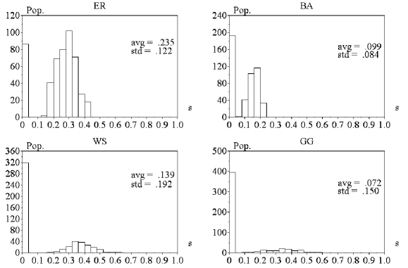
Figure 9: The population histograms of the separation index $s$ for the four considered theoretic models of complex networks with $N=100$, $M=3$ and $\left<k\right>=6$. A substantial decrease of the attractors separation has been implied in all cases. 

Because the last configuration exhibited an accentuated loss of separability because of lack of space in the network, it is interesting to reconsider the effect of increasing $N$ for this situation. The results obtained for the same previous configuration, but now with $N=200$, are shown in Figure 10. The separation index increased substantially for all the four network models. It could be expected that such improvements tend to decrease for still larger $N$, until reaching a regime where little improvement is observed. In such a state, the prototype nodes would be sufficiently far away one another so that their separation no longer depends on $N$. Additional investigation about the change of the average and standard deviation of $s$ are to be found in Section IV.3.

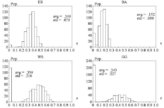
Figure 10: The population histograms of the separation index $s$ for the four considered theoretic models of complex networks with $N=100$, $M=10$ and $\left<k\right>=6$. A substantial decrease of the attractors separation has been implied in all cases. 

Finally, we check for the possible effect of the average node degree on the separation index. Again, the same configuration as the network in Figure 7 is adopted, but now with $\left<k\right>=20$ (i.e. $m=10$) instead of $\left<k\right>=6$. Figure 11 depicts the respectively obtained results, which indicate a clear reduction of the attractors separability. Such an effect is possibly a consequence of the fact that once the network become too intensely connected, the shortest path between the prototype nodes will be reduced and the separability undermined.

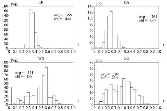
Figure 11: The population histograms of the separation index $s$ for the four considered theoretic models of complex networks with $N=100$, $M=10$ and $\left<k\right>=20$. The effect of increasing the average degree was to substantially decrease the attractors separation in all cases. 

IV.3 Finite Size Effects

The simulations discussed in the previous section seem to have indicated that increases of the value of $N$ would tend to improve the attractors separation until reaching a regime where so much space is available that the patterns no longer feels the finite size of the network. In order to obtain further insights about this effect, the configuration involving $m=3$ and $M=3$ was simulated for $N=50,100,150,200,250$ and the results are given in Figure 12. This figure shows the average (a) and standard deviation (b) of the neighborhood separation index in terms of $N$. It is clear from these results that the increase of $N$ does enhance the attractors separation until reaching a plateau, where a possible ’unsaturation’ occurs, indicating that the finite size effects are over for the specific parameters $m$ and $M$. At the same time, $\sigma(s)$ decreases, also reaching a relatively low plateau. Similar results could be expected for other configurations. In the case of a larger value of $M$, it is expected that $\left<k\right>$ will increase more steeply along the smaller values of $N$, reaching a similar plateau at larger values. Therefore, as the ’unsaturation’ effect was further corroborated by the additional analysis, such a behavior can be considered as a guideline for choosing a proper value of $N$ given $M$ and $m$, for instance by choosing $N$ where $\left<k\right>$ reaches a fixed proportion of its plateau value.

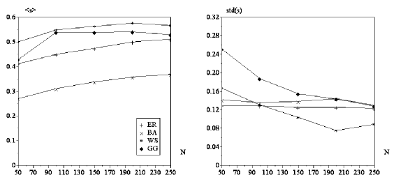
(a)                                     (b)

Figure 12: The average and standard deviation of the neighborhood separation index ($\left<k\right>$ and $\sigma(s)$, respectively) as a function of $N$ for the four models of networks considering $m=3$ and $M=3$. While the averages increase and then tend to a plateau, the standard deviations decrease and also stabilize.  

IV.4 Correlation Analysis

In addition to studying the effects of the involved topologic measurements on the attractors separation, it is also particularly useful to try to identify in which ways the separation index is related to them. This may allow the prediction of the separability without performing dynamic simulation, i.e. by considering only the topologic measurements. Table 1 show the Pearson correlation coefficients obtained considering all pair os topologic measurement (i.e. $\left<cc\right>$, $\left<sp\right>$, $\sigma(sp)$, $Vi$, $\left<mi\right>$, $\sigma(mi)$ and $diam$) and the two separation indices ($s_{ind}$ and $s$).

As previously verified in da F. Costa et al. , the pattern of correlations resulted not similar for each model of network. In addition, the obtained results indicate several high absolute correlation values. In the case of $ER$ networks, the most intense negative correlation (-0.79) was obtained between $\left<sp\right>$ and $\left<mi\right>$, which was indeed expected as longer shortest path lengths tend to reduce the matching index. While similar high correlation (-0.78) was observed also for $BA$, this specific correlation was relatively smaller for the $WS$ and $GG$ cases (-0.50 and -0.42, respectively). This fact was reflected in the intense negative correlation (-0.77) between $s$ and $\left<mi\right>$ and positive correlation (0.63) with $\left<sp\right>$ for the $ER$ model. A similar effect can be observed for the $BA$, $WS$ and $GG$ networks. Observe that $\left<mi\right>$ is highly correlated (0.72 for ER) with $\sigma(mi)$, suggesting a dependence between the standard deviation and average of this measurement. The index quantifying the uniformity of the Voronoi tessellation was found to be negatively correlated with $\left<mi\right>$ and $\sigma(mi)$, as expected, because higher $mi$ values are favored by more irregular Voronoi areas. Interestingly, low correlation values were observed between $s$ and the network diameter and clustering coefficients in all cases. It is also interesting to note that rather different patterns of correlations were obtained between $s_{ind}$ and $s$ and the topologic measurements for all network models.

ER       $s_{ind}$ $s$ $\left<cc\right>$ $\left<sp\right>$ $\sigma(sp)$ $Vi$ $\left<mi\right>$ $\sigma(mi)$ $diam$ $s_{ind}$ 1 $s$ -0.11 1 $\left<cc\right>$ -0.06 -0.11 1 $\left<sp\right>$ -0.51 0.63 -0.11 1 $\sigma(sp)$ 0.31 -0.38 0.07 -0.11 1 $Vi$ -0.17 0.40 -0.03 0.19 -0.19 1 $\left<mi\right>$ 0.51 -0.77 0.08 -0.79 0.49 -0.44 1 $\sigma(m)i$ 0.37 -0.52 0.09 -0.51 0.44 -0.52 0.72 1 $diam$ 0.02 0.00 -0.06 0.03 -0.01 0.10 -0.01 -0.05 1       (a)
BA       $s_{ind}$ $s$ $\left<cc\right>$ $\left<sp\right>$ $\sigma(sp)$ $Vi$ $\left<mi\right>$ $\sigma(mi)$ $diam$ $s_{ind}$ 1 $s$ -0.02 1 $\left<cc\right>$ -0.08 -0.26 1 $\left<sp\right>$ -0.53 0.62 -0.13 1 $\sigma(sp)$ 0.25 -0.10 -0.16 0.01 1 $Vi$ -0.10 0.81 -0.26 0.54 -0.12 1 $\left<mi\right>$ 0.44 -0.69 0.13 -0.78 0.40 -0.65 1 $\sigma(mi)$ 0.47 -0.35 0.06 -0.58 0.28 -0.46 0.61 1 $diam$ 0.03 0.09 -0.24 0.08 -0.08 0.07 -0.06 -0.03 1       (b)
WS       $s_{ind}$ $s$ $\left<cc\right>$ $\left<sp\right>$ $\sigma(sp)$ $Vi$ $\left<mi\right>$ $\sigma(mi)$ $diam$ $s_{ind}$ 1 $s$ -0.58 1 $\left<cc\right>$ -0.04 0.09 1 $\left<sp\right>$ -0.46 0.54 0.10 1 $\sigma(sp)$ 0.43 -0.16 0.06 0.31 1 $Vi$ -0.55 0.63 0.10 0.53 -0.09 1 $\left<mi\right>$ 0.89 -0.80 -0.04 -0.50 0.36 -0.69 1 $\sigma(mi)$ 0.42 -0.54 -0.05 -0.37 0.13 -0.37 0.55 1 $diam$ -0.01 0.02 0.29 0.18 0.16 0.07 -0.02 -0.02 1       (c)
GG       $s_{ind}$ $s$ $\left<cc\right>$ $\left<sp\right>$ $\sigma(sp)$ $Vi$ $\left<mi\right>$ $\sigma(mi)$ $diam$ $s_{ind}$ 1 $s$ -0.16 1 $\left<cc\right>$ -0.06 0.04 1 $\left<sp\right>$ -0.04 0.42 0.13 1 $\sigma(sp)$ 0.16 -0.10 0.11 0.57 1 $Vi$ -0.38 0.71 0.08 0.40 -0.09 1 $\left<mi\right>$ 0.40 -0.87 -0.06 -0.42 0.16 -0.71 1 $\sigma(mi)$ 0.33 -0.72 -0.06 -0.31 0.20 -0.58 0.82 1 $diam$ -0.07 0.04 0.19 0.31 0.30 0.12 -0.10 -0.05 1       (d) .

Table 1: Pearson correlation coefficients obtained for the ER (a), BA (b), WS (c) and GG (d) networks with $N=100$, $m=3$ and $M=3$ considering the individual ($s_{ind}$) and neighborhood ($s_{ngh}$) separability indices and seven measurements of the topology of the network (i.e. average clustering coefficient ($\left<cc\right>$), average shortest path between prototype nodes ($\left<sh_{p}ath\right>$), standard deviation of the shortest paths between the prototype nodes ($\sigma(sh_{p}ath)$)), average Voronoi index ($Vi$), average matching index between prototype nodes ($\left<m\right>$), standard deviation of the matching index between prototype nodes ($\sigma(mi)$) and diameter of the networks (diam)

IV.5 Structural Equation Modeling (SEM) / Path Analysis

Although the correlation analysis described in the previous section can provide interesting information about the pairwise relationship between the separation indices and the topologic measurements, such results are limited because they do not reflect the general relationship between all the topologic measurements and the separation indices. In addition, some of the high observed absolute correlation values can be a consequence of spurious Raykov and Marcoulides (2000); Kline (2005) effects between the variables. In order to gather additional insights about the how the dynamic parameters (i.e. the separation indices) are influenced (and even to a large extent defined) by the topology of the network, while considering all measurement co-variations, we performed path analysis considering the structural dependence between measurements as expressed in Figure 5. It is expected that, by considering all dispersions, the path analysis can provide a more objective and filtered indication of the influences of the topologic measurements on the attractors separation.

The considered data were respective to ER, BA, WS and GG networks with $N=100$, $M=3$ and $m=3$. After estimation of the covariance of the measurements, coding and execution in the LISREL environment, the regression coefficients and residues ($E1$ and $E2$), as well as the relationship between these residuals ($C_{12}$) were obtained. The results are given in Table 2.

A series of interesting insights have been derived from these results. As with the correlations, the dependencies between the topology and separation are strictly specific to each network model, a dependency which may also change for other configurations with different values of the parameters $M$ and $m$. In the case of the ER networks, the standard deviation of the matching index ($\sigma(mi)$) resulted particularly influent (negative influence = -0.96) on the $s$ index. At the same time, the average matching index ($\left<k\right>$) was found to have a strong influence on $s$. Except for relatively smaller negative influence of the $\left<cc\right>$ on $s$, no particularly strong influences are observed with respect to the other topologic measurements. Such a strong influence of the matching index can be understood because non-zero matching index are obtained only in extreme cases, where the prototype nodes are too close. Therefore, nonzero matching indices are a strong and secure indication of poorly separated attractors. For this reason, the matching index dominated the path analysis and implied smaller influences for most other measurements, including the shortest path. This effect can also be observed for the BA and WS cases. However, it is interesting to note the weak influence of $\sigma(mi)$ on $s$ in the case of GG networks. For the BA case, the strongest influence on $s$ was identified for the Voronoi index $Vi$, which is compatible with the fact that higher uniformity of the Voronoi tessellation by the prototype nodes tends to promote better separation between those nodes. Interestingly, a particularly strong influence of $Vi$ on the $s$ has been observed only for the BA model. This effect can be related to the fact that the BA provides the poorest general separation between attractors as a possible consequence of the generalized connectivity implemented by the hubs. In such cases, where a larger number of non-zero matching indices are therefore obtained, the Voronoi separation may become more relevant as a predictor of the separability. In the case of WS models, strong influence (positive = 0.65) was obtained for the $\left<cc\right>$. This effect is particularly interesting because it could be expected that, by promoting smaller shortest paths, this measurement would be inversely related to the separability, which is indeed the case for the respective ER and BA path analysis results. Indeed, a very weak dependency with this variable had been revealed by the Pearson correlations. However, the positive influence of $\left<cc\right>$ on $s$ can be a consequence of the fact that GG networks with higher average clustering coefficients will tend to have more intense local connectivity which could allow the activity to diffuse more uniformly and to concentrate effectively around the prototype nodes. Such an effect would be more definite in the WS case because of the higher uniformity of local connections implied by its ring structure. The influences of the topologic features on the $s$ obtained for the GG cases are dominated by $\left<mi\right>$ as discussed above.

		$\left<cc\right>$	$\left<sp\right>$	$\sigma(sp)$	$Vi$	$\left<mi\right>$	$\sigma(mi)$	$diam$	$Res.$	$C$
ER	$s_{ind}$	$\gamma_{13}=-0.01$	$\gamma_{14}=-0.02$	$\gamma_{15}=0.01$	$\gamma_{16}=-0.01$	$\gamma_{17}=0.01$	$\gamma_{18}=0.01$	$\gamma_{19}=0.00$	$E1=0.00$	$C_{1,2}=0.01$
	$s$	$\gamma_{23}=-0.43$	$\gamma_{24}=0.04$	$\gamma_{25}=-0.03$	$\gamma_{26}=0.25$	$\gamma_{27}=-0.96$	$\gamma_{28}=1.13$	$\gamma_{29}=-0.01$	$E2=0.00$
BA	$s_{ind}$	$\gamma_{13}=-0.02$	$\gamma_{14}=-0.02$	$\gamma_{15}=0.01$	$\gamma_{16}=0.03$	$\gamma_{17}=-0.02$	$\gamma_{18}=0.06$	$\gamma_{19}=0.00$	$E1=0.00$	$C_{12}=0.00$
	$s$	$\gamma_{23}=-0.21$	$\gamma_{24}=0.06$	$\gamma_{25}=0.01$	$\gamma_{26}=0.75$	$\gamma_{27}=-0.39$	$\gamma_{28}=0.73$	$\gamma_{29}=0.00$	$E2=0.00$
WS	$s_{ind}$	$\gamma_{13}=-0.05$	$\gamma_{14}=0.00$	$\gamma_{15}=0.01$	$\gamma_{16}=0.03$	$\gamma_{17}=0.17$	$\gamma_{18}=-0.69$	$\gamma_{19}=0.00$	$E1=0.00$	$C_{12}=0.00$
	$s$	$\gamma_{23}=0.65$	$\gamma_{24}=0.01$	$\gamma_{25}=0.01$	$\gamma_{26}=0.08$	$\gamma_{27}=-0.55$	$\gamma_{28}=-3.54$	$\gamma_{29}=-0.16$	$E2=0.00$
GG	$s_{ind}$	$\gamma_{13}=-0.03$	$\gamma_{14}=0.00$	$\gamma_{15}=0.00$	$\gamma_{16}=-0.02$	$\gamma_{17}=0.05$	$\gamma_{18}=-0.01$	$\gamma_{19}=0.00$	$E1=0.00$	$C_{12}=0.01$
	$s$	$\gamma_{23}=-0.10$	$\gamma_{24}=0.00$	$\gamma_{25}=0.00$	$\gamma_{26}=0.17$	$\gamma_{27}=-0.87$	$\gamma_{28}=-0.08$	$\gamma_{29}=-0.01$	$E2=0.00$

Table 2: The influences of each considered topologic measurement on the attractors separation indices as revealed by path analysis considering $N=100$,$M=3$ and $m=3$.

While the previous path analysis has revealed a series of insights about the influence of the network topology on the dynamic separation of its attraction basins, it was strongly biased by the critical influence of the matching index. In order to try to get further insights on the structure/dynamics relationship for the four considered models, we repeated the path analysis while not including $\left<mi\right>$ and $\sigma(mi)$. The results are summarized in Table 3. Interestingly, except for relatively small increases with respect to $Vi$ and $\left<cc\right>$, the obtained influences remained similar, with small effects observed for the shortest path measurements. This can be understood as a confirmation that the separation between the attractors is critically defined by the overlap between the hierarchical neighbors of the prototype nodes, especially their immediate neighbors (implying higher matching indices). In the cases where the matching index is zero, the lack of congruence between the original attractors and the distribution of diffusive activity should be largely explained by the higher influences observed in Table 3, which involve the average clustering coefficient of the network and the Voronoi index for the prototype nodes. Indeed, in the cases where the prototype nodes are not topologically too close one another, the lack of agreement between the activity distribution and the original attractors (as in Figure 1b and c) will depend particularly on the properties of the local connectivity as expressed by the clustering coefficient and the node degree.

		$\left<cc\right>$	$\left<sp\right>$	$\sigma(sp)$	$Vi$	$diam$	$Res.$	$C$
ER	$s_{ind}$	$\gamma_{13}=-0.01$	$\gamma_{14}=-0.02$	$\gamma_{15}=0.01$	$\gamma_{16}=-0.01$	$\gamma_{17}=0.00$	$E1=0.00$	$C_{12}=0.00$
	$s$	$\gamma_{23}=-0.26$	$\gamma_{24}=0.14$	$\gamma_{25}=-0.09$	$\gamma_{26}=0.43$	$\gamma_{27}=-0.01$	$E2=0.00$
BA	$s_{ind}$	$\gamma_{13}=-0.02$	$\gamma_{14}=-0.02$	$\gamma_{15}=0.01$	$\gamma_{16}=0.03$	$\gamma_{17}=0.00$	$E1=0.00$	$C_{12}=0.00$
	$s$	$\gamma_{23}=-0.22$	$\gamma_{24}=0.08$	$\gamma_{25}=-0.01$	$\gamma_{26}=0.79$	$\gamma_{27}=-0.00$	$E2=0.00$
WS	$s_{ind}$	$\gamma_{13}=0.03$	$\gamma_{14}=-0.01$	$\gamma_{15}=0.01$	$\gamma_{16}=-0.05$	$\gamma_{17}=0.00$	$E1=0.00$	$C_{12}=0.00$
	$s$	$\gamma_{23}=0.43$	$\gamma_{24}=0.03$	$\gamma_{25}=-0.03$	$\gamma_{26}=0.41$	$\gamma_{27}=-0.01$	$E2=0.00$
GG	$s_{ind}$	$\gamma_{13}=-0.01$	$\gamma_{14}=0.00$	$\gamma_{15}=0.0$	$\gamma_{16}=-0.04$	$\gamma_{17}=0.00$	$E1=0.00$	$C_{12}=0.01$
	$s$	$\gamma_{23}=-0.21$	$\gamma_{24}=0.04$	$\gamma_{25}=-0.03$	$\gamma_{26}=0.51$	$\gamma_{27}=-0.01$	$E2=0.00$

Table 3: The influences of each considered topologic measurement on the attractors separation indices as revealed by path analysis considering $N=100$,$M=3$ and $m=3$.

V Conclusions

The investigation about the relationship between the structure and function of networks (e.g. Newman (2003); Boccaletti et al. (2006); da F. Costa (2005a)) represents one of the most interesting perspectives for obtaining insights about complex dynamic systems. As briefly reviewed in this article, several works have addressed the problem of how the structure of the connectivity may affect and largely define the properties of dynamic systems. One particularly important aspect which has received relatively lesser attention concerns the separability between different grandmother attractors, each representing a prototype pattern or state. This issue is critically relevant because it has great impact on the capacity of the network for proper representation of patterns, the level of redundancy/robustness of such representations, the degree of generalization for recognition of not previously trained prototypes, as well as the effectiveness during retrieval and activation of such prototypes. While other types of coding can be used in dynamic system, grandmother representation stands out as particularly important because it seems to be the way a great part of the primates cortex is organized.

The current work has reported an approach to the characterization of the separability between prototype patterns which incorporates a number of special features. First, we have considered four representative theoretic models of complex networks – namely the random networks of Erdő-Rényi, the scale free model of Barabási-Albert, the small-world networks of Watts-Strogatz, as well as a simple, non-small-world topographic model. Second, by using a generic diffusive process, followed by the calculation of the respective derivative network in order to obtain the attraction basins, we obtained a methodology which completely avoids the intricacies and specifities implied by each type of dynamic system. While it remains to be verified how good accurate and general such an approximation is, it does allow the definition of smooth attraction basins around each prototype node in a way which is remindful of many important dynamical systems such as Kohonen’s self-organizing maps and the primates cortex. Once the attraction basins are so defined, a simple diffusive scheme emanating from each network node is employed in order to obtain the general activation of the network. Although ideally such a procedure should activate equally only the original prototype nodes, the structured connectivity of the networks will act so as to produce non-uniform activation, where just a fraction of the overall activation coincides with the prototype nodes. The disagreement between the original prototypes and the induced activity has been quantified in terms of two separation indices, namely the individual and neighborhood indices. Because the former consider only the agreement and balance between the induced activation and the original prototypes, it resulted to be too small and therefore with low resolution for quantifying the attractors separation. By considering also the immediate neighborhood of the prototype nodes, the second index allowed a more informative indication of the attractors separability.

The specific topologic features of each of the four considered theoretic network models can have different effects for the separation of the attraction basins. Therefore, we performed an investigation of the effects of the most important parameters of the simulations over the respective performance. We verified that the separation tends to decrease with the number of prototypes and increase with the size of the network. At the same time, more intense general connectivity, as expressed by the average node degree, also tended to undermine the attractors separation. Special attention was given to the finite sizes implied by the parameter $N$. The obtained results seem to suggest that the separability tends to increase with $N$ up to a regime where the finite size of the network is no longer felt (‘unsaturation’). Therefore, by identifying the region where such a plateau of separability is reached, it is possible to obtain near-optimum values of $N$ for given $M$ and $m$. Next, we applied correlation analysis in orde not only to identify the inter-relationships between each topologic measurement, but also between these and the two separation indices. The presence of such correlations can not only help to understand the origin of the attractors separation, but also allow the prediction of such a property from measurements of the network topology, without the need of simulations. Several tendencies were identified through such an analysis, including the tendency of the index $s$ to be strongly proportional to the uniformity of the Voronoi areas, as expressed by the Voronoi index $Vi$. A positive, though weaker, correlation was also identified between $s$ and the average shortest path length $\left<sp\right>$ of the networks. A strong negative correlation was identified between $s$ and the matching index $mi$. Although all such behaviors are compatible with what could be expected, meaningfully different correlations differences were observed for each network model. Interestingly, the network model allowing the best overall separation of attractors was found to be the Watts-Strogatz, followed by the geographic, random and scale-free models. It is conjectured here that the superior properties of the WS model stem from its enhanced uniformity and low randomness of local connectivity as well as by the fact that, although being a small world model, there are relatively very few long range connections between any pair of nodes. Similar properties, though at the expense of a weaker local order and uniformity of local connections, are characteristic of the geographic model, which came in second in performance. As a matter of fact, the WS and GG models showed similar behavior as far as the histograms of separation index were concerned. The same was observed for the ER and BA cases. Therefore, from the perspective of attractors separation, the WS/GG and ER/BA models seem to represent two different classes of systems, with the latter providing rather poorer separability. Interestingly, the small world property can not explain such a partition, as the GG is not a small world model as the other three cases. Consequently, it seems that the common denominators in the pairs WS/GG and ER/BA seems to be more strongly related also to the uniformity of the local connectivity. Such an explanation would be largely in agreement with several of the results of works investigating the effect of connectivity on memory, as reviewed in Section II.

In order to try to learn more about the effects of the topological features of the network on the dynamical property of attractors separation, path analysis was also applied assuming a simple structural relationship. To our best knowledge, this is the first time such an insightful analysis has been applied for the study of complex networks. One of the main advantages of such an approach over the Pearson correlation coefficients is that here the dispersions of all the considered measurements are taken into account instead of the pairwise relationships underlying the correlations. Interestingly, the path analysis yielded influences of the topologic measurements on the separation indices which were often substantially different from those suggested by the Pearson correlation coefficients. Of particular interest was the near null influence assigned to the average and standard deviation of the shortest path length between the prototype nodes. This is all the most surprising as it seems intuitively reasonable to discuss much of the effect of the topology of the network over the attractors separation by considering such measurements. More specifically, networks where the prototype nodes are topologically close one another would tend to have poorer separation. However, the performed path analysis substantially emphasized, for all the four considered models, the importance of the average matching index on the attractors separation. On second thoughts, this is indeed reasonable because the presence of non-zero matching index is a certain indication of overlap of the attraction basins. Even when repeating the path analysis while leaving out the matching index measurements, the other parameters (especially the shortest path length) did not result with higher influences. Other interesting insights, including influences which were specific to network models, were also allowed by the path analysis, corroborating therefore the potential value of such a statistical approach in order to get insights about the relationship between structure and dynamics of complex dynamic systems. However, it is important to keep in mind that every statistical methodology should be understood as a source of insights to be further investigated and corroborated rather than spelling definitive facts.

Despite the relative comprehensiveness of the presently reported investigation, and perhaps as its consequence, a series of future developments can be suggested. First, it would be interesting to extend the reported investigation to larger network sizes and to consider additional measurements such as the standard deviation of the clustering coefficient and the spectral structure of the adjacency and weight matrix. Second, the sources of the deviations of the induced activation from the prototype nodes could be further investigated by considering simulations involving a single attractor. In such cases, all the loss of ‘separability’ would necessarily be a consequence of the probability leakage from the prototype node into its neighbors. It would be particularly interesting to verify, through path analysis, which of the topological measurements of the network would be more influence on the attractor activation. It would also be worth investigating the potential of using the percolation transform da F. Costa (2004c, 2005c) over the network as the means to explain and predict the attractors separability. Other promising possibilities include the extension of the matching index to take into account hierarchical levels larger than one, i.e. including also the second and higher neighborhoods.

Several real problems are closely related to the issue of attractor separation and prototype activation. One real problem which could be particularly interesting to be addressed is the phenomenon of facilitation of neurons (represented by nodes). By facilitation of a neuron it is meant that that neuron will become more likely to engage into activity. For instance, the definition of temporary priorities in the primates brain could be related to the reinforcement of one or more attractors, so that they become more likely to be revised along time (e.g. through a random walk). Interestingly, as suggested by the current work, the facilitation of a given node would be highly dependent on its local connectivity. Such studies could be eventually extended to higher level mental dynamics, such as those underlying attention and even pathologies (e.g. Wedemann et al. (2006)). It is also reasonable to expect that the definition of attractors is a process which co-evolves with the network topology. In this sense, it would be interesting to try to identify growing schemes where the connectivity is affected by the success of the establishment of prototype attractores, and vice-versa. Another related investigation would be the identification of topologic organizations of networks allowing optimal or near-optimal attractors separation.

List of Symbols

$\Gamma=$ a graph or complex network;

$N=$ number of nodes in a network;

$K=$ the adjacency matrix of a complex network;

$k(i)=$ degree of a network node $i$;

$m=$ the parameter in the BA model defining its average node degree. This parameter is considered as reference for all network models in this work;

$diam=$ the diameter of the network;

$cc(i)=$ clustering coefficient of a network node $i$;

$sp(i,j)$ shortest path between nodes $i$ and $j$ in a complex network;

$mi(i,j)=$ the matching index of nodes $i$ and $j$;

$Vi=$ the Voronoi index of separation between the areas of influence of the prototype nodes;

$\left<a\right>=$ the arithmetic average of the property $a$;

$\left[a\right]=$ the geometric average of the property $a$;

$\sigma(a)=$ the standard deviation of the random variable $a$;

$M=$ the number of prototype patterns to be represented in a network;

$\vec{\alpha}=$ the activations in a network after a long random walk;

$s_{ind}=$ the separability index between prototype nodes in a network at the level of individual nodes;

$s=$ the separability index between prototype nodes in a network considering also the immediate neighborhood of such nodes;