Stochasticity and Non-locality of Time
Abstract
We present simple classical dynamical models to illustrate the idea of introducing a stochasticity with non-locality into the time variable. For stochasticity in time, these models include noise in the time variable but not in the “space” variable, which is opposite to the normal description of stochastic dynamics. Similarly with respect to non-locality, we discuss delayed and predictive dynamics which involve two points separated on the time axis. With certain combinations of fluctuations and non-locality in time, we observe a “resonance” effect. This is an effect similar to stochastic resonance, which has been discussed within the normal context of stochastic dynamics, but with different mechanisms. We discuss how these models may be developed to fit a broader context of generalized dynamical systems where fluctuations and non-locality are present in both space and time.
1 Introduction
“Time” is a concept that has drawn a lot of attention from thinkers in virtually all disciplines [1]. In particular, our ordinary perception is that space and time are not the same, and this difference appears in various contemplations of nature. It appears to be the main reason for the theory of relativity, which has conceptually brought space and time closer to receiving equal treatment, and it continues to fascinate and attract thinkers from diverse fields. Moreover, issues such as the “direction” or the “arrow” of time [2] and complex time [3] are current research interests.
It seems that there are other manifestations of this difference. One is the treatment of noise or fluctuations in dynamical systems. Time in dynamical systems, whether they are classical, quantum, or relativistic, is commonly viewed as not having stochastic characteristics. In stochastic dynamical theories, we associate noise and fluctuations with only “space” variables, such as the position of a particle, and not with the time variable. In quantum mechanics, the concept of time fluctuation is embodied in the time-energy uncertainty principle. However, time is not treated as a dynamical quantum observable, and clear understanding of the time-energy uncertainty has yet to be found [4].
Another difference seems to show up in our cognition of non-locality in space and time. Non-local effects in space are incorporated in physical theories describing wave propagation, fields, and so on. In quantum mechanics, the issue of spatial non-locality is more intricate, constituting the backbone of such quantum effects as the Einstein-Podolsky-Rosen paradox [5]. With respect to time, there have been investigations of memory effects in dynamical equations. However, less attention has been paid to non-locality in time, and behaviors associated with non-locality in time, such as delay differential equations, are not yet fully understood [6, 7, 8, 9].
Against this background, the main topic of this paper is to consider stochasticity and non-locality of time in classical dynamics through a presentation of simple models. We discuss delayed and predictive dynamics as examples of non-locality in time. For stochastitiy, we present a delayed dynamical model with fluctuating time, or stochastic time. We shall see that this combination of stochasticity and non-locality in time can exhibit behaviors which are similar to stochastic resonance [10, 11, 12], which arises through a combination of oscillating behavior and “spatial” noise and has been studied in variety of fields [13, 14, 15, 16, 17].
2 Delayed and Predictive Dynamics
We start with a consideration of non-locality of time in classical dynamical models. The general differential equation of the class of dynamics we discuss here is as follows.
| (1) |
Here, is a dynamical variable of time , and is the “dynamical function” governing the dynamics. Its difference from the normal dynamical equation appears in , which can be either in the past or the future, and in general. In other words, the change in is governed by , not its “current” state , but its state at . We can define and , as well as the function , in a variety of ways. In the following, we will present two cases: delayed and predictive dynamics.
Delayed dynamics can be obtained from the general definition by
| (2) |
Here, is the delay, and the dynamics depend on two points on the time axis separated by . Delayed dynamical equations have been studied for various applications [6, 7, 8, 9].
Predictive dynamics, on the other hand, have recently been proposed [18, 19] and, they take in the future, i.e., . We call an “advance”. We also need to define the state of the dynamical variable at this future point in time. Here, we estimate such that
| (3) |
This prediction is termed “fixed rate prediction”. Namely, we estimate as the value that would be obtained if the current rate of change extends for a duration from the present point to the future point. Qualitatively, this is one of the most commonly used methods for estimating population, national debt, and so on.
We also note that there are studies of equations called “functional differential equations of the advanced type”, or “advanced functional differential equations” [20, 21, 22]. They also are differential equations with advanced arguments, and we can obtain equations of this class from our general definition by setting,
| (4) |
with suitably chosen boundary conditions. The predictive dynamical equations differ from this class of equations, as we allow flexibility in defining based on a prediction scheme.
We shall investigate the properties of these delayed and predictive dynamical models through computer simulations. To avoid ambiguity and for simplicity, we will study time-discretized map dynamical models, which incorporate the above–mentioned general properties of the delayed and predictive dynamical equations.
| (5) |
Here, is a parameter controlling the rate of change. For a delayed map with a delay , we define
| (6) |
while for the predictive map with an advance , we have
| (7) |
We choose the Mackey-Glass function as the dynamical function (Fig. 1), i.e.,
| (8) |
where and are parameters. This function was first proposed for modeling the cell reproduction process and is known to induce chaotic behavior with a large delay [6].
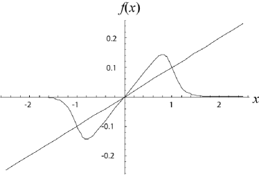
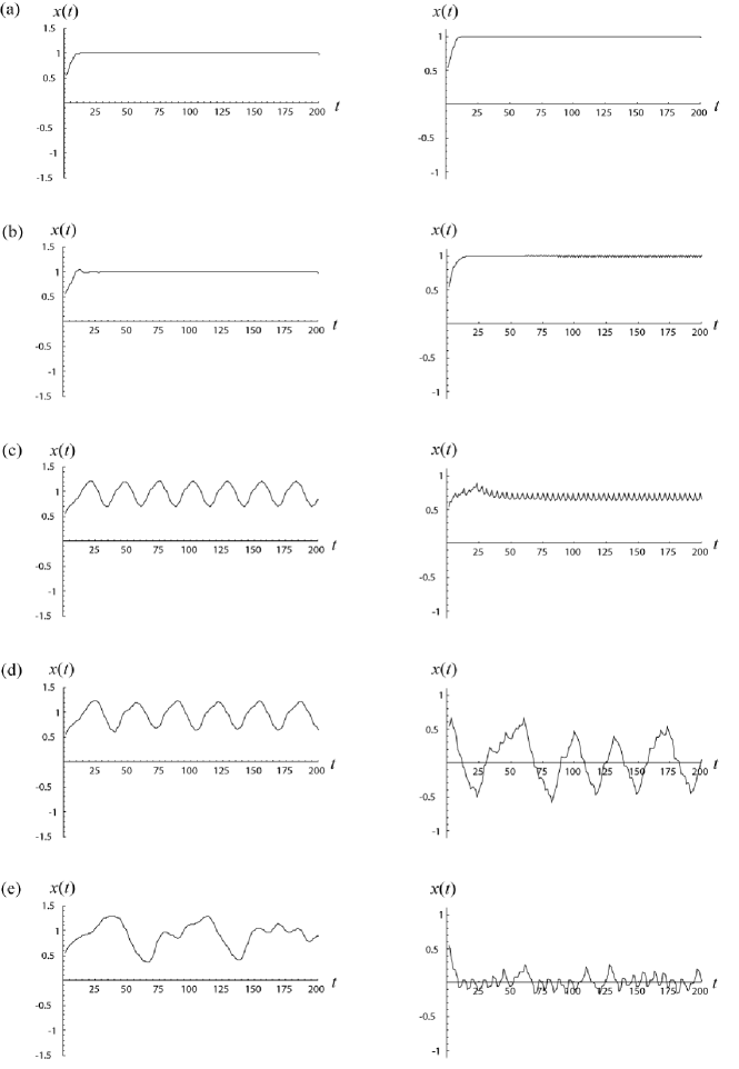
Figure 2 shows examples of computer simulations of the delayed and predictive cases. The parameters are set so that without a delay or advance, , the model monotonically approaches the stable fixed point. The stability of the fixed point is lost as , or , increases, giving rise to complex dynamics. Thus, non-locality in time can induce a complex behavior in otherwise simple dynamical systems.
Now, we would like to make a few remarks. First, in the case of delayed dynamics, we need to decide on the initial function and delay. Analogously, in predictive dynamics, the prediction scheme and advance need to be specified. Common to delayed and predictive dynamical systems, both factors affect the nature of the dynamics.
In addition, we can use linear stability analysis on both the delayed and predictive cases. This analysis can give an estimate of the critical delay or advance at which the stability of the fixed point is lost. However, the nature of the dynamics beyond these critical points is not yet clearly understood.
For the case of delayed dynamics, with the addition of a suitable “strength” of noise, a behavior similar to stochastic resonance has been obtained [23]. This phenomenon, called “delayed stochastic resonance,” has a different mechanism in the sense that it does not require external oscillatory signals or forces, but instead it uses a delay as the source of the oscillation to be combined with noise. An analogous resonance phenomenon has been observed in predictive dynamics with added noise, which is termed “predictive stochastic resonance”[19].
3 Stochastic Time
We now turn our attention to the fluctuation of time, which we term “stochastic time” in the context of classical dynamical systems. As in non-locality, there are various ways to bring in stochasticity. We have found that stochastic time combined with delayed dynamics leads to phenomena similar to stochastic resonance.
The general differential equation of the class of delayed dynamics with stochastic time is given as
| (9) |
Here, as in the previous section, is the dynamical variable of time , and is the “dynamical function” governing the dynamics. is the delay. The difference from the normal delayed dynamical equation appears in , which now contains stochastic characteristics, and these can be introduced in various ways. We will again focus on the following dynamical map system incorporating the basic ideas of the general definition given above.
| (10) |
Here, is the stochastic variable which can take either or with certain probabilities. We associate “time” with an integral variable . The dynamics progress by incrementing integer , and occasionally “goes back” a unit with the occurrence of . Let the probability of be for all , and we set . Then, with , this map naturally reduces to a normal delayed map with . We update the variable with the larger . Hence, in the “past” could be “re-written” as decreases with probability .
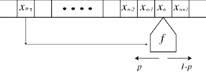
We can make an analogy of this model with a tele–typewriter or a tape–recorder, which occasionally moves back on a tape. Figure 3 gives a schematic view. Based on the values of and , the recording device writes on the tape the values of at a step, and “time” is associated with positions on the tape. When there is no fluctuation (), the head moves only in one direction on the tape and it records values of for a normal delayed dynamics. With probability , it moves back a unit of “time” to overwrite the value of . The question is how the recorded patterns of on the tape are affected as we change .
We will keep the Mackey-Glass function as the dynamical function, and the map model becomes
| (11) |
where , , and are parameters. With both positive, and no stochasticity in time, this map has a stable fixed point with no delay. Linear stability analysis around the fixed point gives the critical delay , at which the stability of the fixed point is lost.
| (12) |
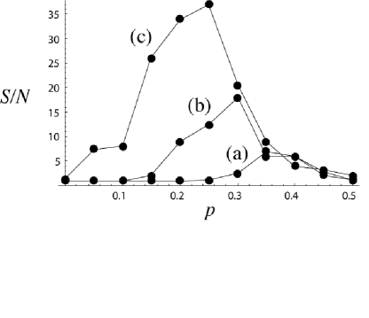
A larger delay gives an oscillatory dynamical path. We have found, through computer simulations, that an interesting behavior arises when the delay is smaller than this critical delay. The tuned noise in the time flow gives the system a tendency for oscillatory behavior. In other words, by adjusting the value of controlling , one induces oscillatory dynamical paths. Some examples are shown in Figure 4. (The critical delay is with the set of parameters.) With increasing probability for a time flow to reverse, i.e., with increasing , we observe oscillatory behavior in the sample dynamical path as well as in the corresponding power spectrum. However, as increases further, the oscillatory behavior begins to deteriorate. In order to see this, we compute the “signal–to–noise” () ratio by using the ratio of the peak height to the background in the spectrum. Figure 5 illustrates this change in , which reaches a maximum at an appropriately “tuned” value of .

Again, we see a phenomenon which resembles stochastic resonance. A theoretical analysis of the mechanism of our model is yet to be done. In particular, we note that the model has an intricate mixture of time scales of delay, the oscillation period of , and stochastic time. These factors are likely to be involved in the time scale analysis [24], but we leave consideration of them for the future. On the other hand, this resonance with stochastic time is clearly of a different type and new. We discussed only the Mackey–Glass function for consistency, but the same behavior is also observed in other delayed dynamical systems, such as ones with a negative feedback function [25].
We have also studied predictive dynamics with stochastic time, but so far, have not found behaviors similar to this resonance with delayed dynamics. Yet, the example above with delayed dynamics indicates that a combination of stochasticity and non-locality in time may lead to entirely new phenomena.
4 Discussion
We could extend our model so that we have a picture of dynamical systems with stochasticity and non-locality on the time and space axes. The analytical framework and tools for such descriptions need to be developed, along with a search for appropriate applications.
An example of an appropriate application of temporal non-locality is modeling a stick balancing on a human fingertip. Recent experiments have found that most of the observed corrective motions occur on shorter time scales than that of the human reaction time [26, 27, 28]. This may be the result of intricate mixtures of physiological delays, predictions, and physical fluctuations. Models incorporating special fluctuations and delays have been considered, but none have tried to include the effect of prediction.
Another direction of development might be to extend the path integral formalism to allow stochastic time paths. The question of whether this extension bridges to quantum mechanics and/or leads to an alternative understanding of such properties as the time-energy uncertainty relations requires further investigation.
Finally, if these models can capture some aspects of reality, particularly with respect to temporal stochasticity, this resonance may be used as an experimental indication for probing fluctuations or stochasticity in time. We have previously proposed “delayed stochastic resonance”[23], a resonance that occurs through the interplay of noise and a delay. It was theoretically extended [29], and recently, it was experimentally observed in a solid-sate laser system with a feedback loop [30]. We leave it for the future to see if an analogous experimental test could be developed with respect to stochasticity and non-locality of time.
References
- [1] P. Davies, About Time (Simon and Schuster, New York, 1995).
- [2] S. F. Savitt, Time’s Arrows Today (Cambridge Univ. Press, Cambridge, 1995).
- [3] M. S. El Naschie, Chaos, Solitons and Fractals 5, 1031–1032 (1995).
- [4] P. Busch, in Time in Quantum Mechanics (J. G. Muga, R. Sala Mayato and I. L. Egusquiza, eds. ) 69-98 (Springer-Verlag, Berlin, 2002).
- [5] J. J. Sakurai, Modern Quantum Mechanics (Benjamin/Cummings, Menlo Park, 1985).
- [6] M. C. Mackey and L. Glass, Science 197, 287–289 (1977).
- [7] K. L. Cooke and Z. Grossman, J. Math. Anal. and Appl. 86, 592–627 (1982).
- [8] J. G. Milton, et al., J. Theo. Biol. 138, 129–147 (1989).
- [9] J. G. Milton, Dynamics of Small Neural Populations (AMS, Providence, 1996).
- [10] K. Wiesenfeld, and F. Moss, Nature 373, 33–36 (1995).
- [11] A. R. Bulsara and L. Gammaitoni, Physics Today 49, 39–45 (1996).
- [12] L. Gammaitoni, P. Hänggi, P. Jung, and F. Marchesoni, Rev. Mod. Phys. 70, 223–287 (1998).
- [13] B. McNamara, K. Wiesenfeld and R. Roy, Phys. Rev. Lett. 60, 2626–2629 (1988).
- [14] A. Longtin, A. Bulsara and F. Moss, Phys. Rev. Lett. 67, 656–659 (1991).
- [15] J. J. Collins, C. C. Chow and T. T. Imhoff, Nature 376, 236–238 (1995).
- [16] F. Chapeau-Blondeau, Sign. Process 83, 665–670 (2003).
- [17] I. Y. Lee, X. Liu, B. Kosko and C. Zhou, Nano Letters 3, 1683–1686 (2003).
- [18] T. Ohira, arXiv:cond-mat/0605500.
- [19] T. Ohira, arXiv:cond-mat/0610032 (To appear in the AIP Conf. Proc. of 9th Granada Seminar (Granada, Spain, Septemper 11-15, 2006))
- [20] T. Kusano, Hiroshima Math. J. 11, 617–620 (1981).
- [21] V. B. Kolmanovskii, A. D. Myshkis, Applied theory of functional differential equations, (Kluwer Acad. Publ., Dordrecht, 1995).
- [22] R.P. Agarwal, M. Bohner and W.T. Li, Nonoscillation and oscillation theory for functional differential equations, (Marcel Dekker, New York, 2004).
- [23] T. Ohira and Y. Sato, Phys. Rev. Lett. 82, 2811–2815 (1999).
- [24] J. L. Cabrera, J. Gorro ogoitia and F. J. de la Rubia, Phys. Rev. E 66 022101 (2002).
- [25] T. Ohira, arXiv:physics/0609206 (To appear in the AIP Conf. Proc. of 8th Int. Symp. of Frontiers of Fundamental Physics (Madrid, Spain, October 17-19, 2006)).
- [26] J. L. Cabrera and J. G. Milton, Phys. Rev. Lett. 89 158702 (2002).
- [27] J. L. Cabrera and J. G. Milton, Chaos 14, 691-698 (2004).
- [28] J. L. Cabrera, et al., Fluc. Noise Lett. 4, L107–117 (2004).
- [29] L.S. Tsimring and A. Pikovsky, Phys. Rev. Lett. 87 250602 (2001).
- [30] C. Masoller, Phys. Rev. Lett. 88 034102 (2002).