Long Term Economic Relationships from Cointegration Maps

Abstract

We employ the Bayesian framework to define a cointegration measure aimed to represent long term relationships between time series. For visualization of these relationships we introduce a dissimilarity matrix and a map based on the Sorting Points Into Neighborhoods (SPIN) technique, which has been previously used to analyze large data sets from DNA arrays. We exemplify the technique in three data sets: US interest rates, monthly inflation rates and gross domestic product growth rates.

1 Introduction

Correlations are a central topic in the study of the collective properties of complex systems, being of particularly practical importance when systems of economic interest are concerned [1]. Unlike correlation, the idea of cointegration [2, 3] brings in a relationship measure that is long term in nature being somewhat related to the concept of damage spreading in a pair of spin models [4]. However, cointegration has up to now been rather absent from the description of physical systems and, in particular, from economic systems studied from a physical perspective. A set of non-stationary time series cointegrate if there exists a linear combination of them that is mean reverting. Plainly speaking, two appropriately scaled time series cointegrate if in the long term they either tend to move together or as mirror images.

Bayesian methods provide a unifying approach to statistics [5]. They help to establish, from clear first principles, the methods, assumptions and approximations made in a particular statistical analysis. A major issue in the study of cointegration is the detection of cointegrated sets, a problem that has been extensively dealt with in the econometrics literature both from classical [6] and Bayesian [7] perspectives.

Dealing with extensive volumes of data is a common trend in several areas of science. The need to sort, cluster, organize, categorize, mine or visualize large data sets brings a perspective that unifies distant fields, if not at all in aims, at least in methods. Cross fertilization may promptly provide candidate solutions to problems, avoiding the need of rediscovery or worst, just plain non-discovery. Bioinformatics presents a good example, where the availability of genome, protein and DNA array data has prompted the proposal by several groups of new methods. From this repertoire we borrow a method, SPIN [8], previously developed for automated discovery of cancer associated genes.

Our first goal in this paper is to devise a cointegration measure for time series of economic interest that is both physically meaningful and reasonably simple to compute. Our second goal is, by employing the SPIN method, to emphasize the importance of visual organization and presentation of relationship pictures (or maps) that emerge when complex systems are analysed.

This paper is organized as follows. In the next section we derive a cointegration measure employing Bayesian statistics and briefly discuss the relation between cointegration and correlation and between the proposed measure and usual unit-root statistics. In section 3 we use the SPIN method to introduce the cointegration heat map as a visualization tool. In section 4 we exemplify the proposed technique in three macroeconomic time series: US interest rates (USIR), inflation rates (IFR) and gross domestic products (GDP). Conclusions are presented in section 5.

2 Cointegration measure

A pair of time series ${\bm{x}}_{1}$ and ${\bm{x}}_{2}$ cointegrates [3] if there exists a linear combination

$$a_{1}x_{1,t}+a_{2}x_{2,t}+b = \epsilon_{t}$$ (1)

such that the residues ${\bm{\epsilon}}$ satisfy the following stationarity condition:

$$\epsilon_{t+1} = \gamma\epsilon_{t}+\eta_{t},$$ (2)

where $\langle\eta_{t}\rangle=0$, $\langle\eta_{t}^{2}\rangle=\sigma^{2}$ and $\gamma<1$. If $\gamma=1$ the residues are non-stationary and if $\gamma>1$ the system is unstable. Notice that $\gamma$ is related to a time scale $\tau=1/(1-\gamma)$ for relaxation of $\epsilon_{t}$ to its long term mean.

We also assume a budget constraint taking the form

$$a_{1}^{2}+a_{2}^{2} = 1.$$ (3)

Since eq. 1 is linear, we can impose this constraint by assuming that $a_{1}=\sin(\theta)$ and $a_{2}=\cos(\theta)$ without loss of generality. Note that the above system has still more freedom arising from the following symmetry group:

$$x_{i} \rightarrow x_{i}^{\prime}=\alpha x_{i}+y_{i},$$

$$b \rightarrow b^{\prime}=\alpha b-a_{1}y_{1}-a_{2}y_{2},$$

$$\sigma \rightarrow \sigma^{\prime}=\alpha\sigma,$$

$$\gamma \rightarrow \gamma^{\prime}=\gamma,$$ (4)

which means that we can change the units in which quantities are measured and add constants $y_{i}$ without interfering with the cointegration property. We, therefore, can partially fix the gauge so that $x_{i}\rightarrow x_{i}^{\prime}=x_{i}-\overline{x_{i}}$, such that the empiric time series averages are zero. This forces a choice of $b=0$.

That cointegration and correlation in time series fluctuations are quite distinct properties can be easily seen with the aid of an elementary example. Suppose two time series $x_{t}$ and $y_{t}$ that orbit the same random walk $w_{t}$ as follows:

$$x_{t} = w_{t}+\epsilon^{x}_{t}$$ (5)

$$y_{t} = w_{t}+\epsilon^{y}_{t}$$

$$w_{t} = w_{t-1}+\eta_{t},$$

where $\epsilon^{x}_{t}$, $\epsilon^{y}_{t}$ and $\eta$ are random i.i.d shocks with zero mean and variances $\sigma^{2}_{x}$, $\sigma^{2}_{y}$ and $\sigma^{2}_{\eta}$, respectively. The correlation $\rho$ between the first differences $\Delta x=x_{t}-x_{t-1}$ and $\Delta y=y_{t}-y_{t-1}$ can be easily computed yielding:

$$\rho = \frac{\langle\Delta x\Delta y\rangle}{\sigma_{x}\sigma_{y}}=\frac{\sigma^{2}_{\eta}}{\sigma_{x}\sigma_{y}}.$$ (6)

Clearly $x$ and $y$ strongly cointegrate ($\gamma=0$). However the choice $\sigma_{\eta}\ll\sigma_{x},\sigma_{y}$ would imply that the linear correlation in their fluctuations are at the same time very low.

The main ingredients in a Bayesian approach are three. First we need a model as given by eqs. 1, 2 and 3. Then a noise model to build the likelihood and finally the priors. The interesting consequence of a group of invariance as the one described by eq. 4 is that it, together with the budget and stability conditions, constrains [5] the form of the priors to:

$$p(\gamma) = \Theta(\gamma)\Theta(1-\gamma),$$ (7)

where $\Theta(\cdot)$ is the Heaviside step function, and

$$p(\sigma) \propto \frac{1}{\sigma^{2}}.$$ (8)

With these ingredients we can calculate the posterior probability of $\gamma$ given the residues as:

$$p(\gamma\mid{\bm{\epsilon}}) \propto \int_{\sigma_{\mbox{\tiny min}}}^{\infty}d\sigma\;p({\bm{\epsilon}}\mid\gamma,\sigma)p(\sigma)p(\gamma),$$ (9)

where $\sigma_{\mbox{\tiny min}}>0$ can be made arbitrarily small without changing the main results to follow.

Equations 1 and 2 combined give the following likelihood function for the residues:

$$p(\bm{\epsilon}\mid\gamma,\sigma) \propto \prod_{t=1}^{T-1}\frac{1}{\sigma}\exp\left[-\frac{\left(\epsilon_{t+1}-\gamma\epsilon_{t}\right)^{2}}{2\sigma^{2}}\right].$$ (10)

Performing the integral in eq. 9 yields:

$$p(\gamma\mid{\bm{\epsilon}})\propto\Theta(\gamma)\Theta(1-\gamma)\left[\sum_{t=1}^{T-1}\left(\epsilon_{t+1}-\gamma\epsilon_{t}\right)^{2}\right]^{-\frac{T-2}{2}}.$$ (11)

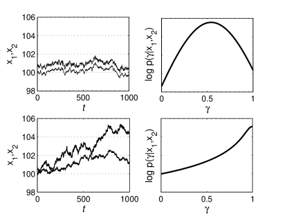
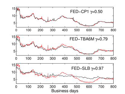
Figure 1: Left: Posterior probabilities for two synthetic pairs ${\bm{x}}_{1},{\bm{x}}_{2}$ of time series. Cointegrating pair, characterized by the maximum a-posteriori estimate $\hat{\gamma}\approx 0.5$ (top). Non-cointegrating pair characterized by $\hat{\gamma}\approx 1$ (bottom). Right: Examples of the cointegration measure in US interest rate data.

For large $T$, the distribution of residues, given the data, can be approximated by

$$p(\bm{\epsilon}\mid{\bm{x}}^{\prime}_{1},{\bm{x}^{\prime}}_{2}) \approx \delta(\epsilon_{t}-x^{\prime}_{1,t}\sin\hat{\theta}+x^{\prime}_{2,t}\cos\hat{\theta})$$ (12)

with $\hat{\theta}$ estimated by minimizing the variance $\langle\epsilon^{2}\rangle$ to find:

$$\hat{\theta} = \frac{1}{2}\arctan\left[2\frac{\langle x^{\prime}_{1}x^{\prime}_{2}\rangle}{\langle{x^{\prime}_{1}}^{2}\rangle-\langle{x^{\prime}_{2}}^{2}\rangle}\right].$$ (13)

The maximum of the posterior distribution gives an estimate for the relaxation time as

$$\hat{\gamma} = \mbox{argmax}\log p(\gamma\mid{\bm{x}^{\prime}}_{1},{\bm{x}^{\prime}}_{2})$$

$$= \mbox{argmax}\log\int d\bm{\epsilon}\,p(\gamma\mid{\bm{\epsilon}})p(\bm{\epsilon}\mid{\bm{x}}^{\prime}_{1},{\bm{x}^{\prime}}_{2}).$$

Finally, we define a family of cointegration $\alpha$-measures as

$$d_{\alpha}({\bm{x}}_{1},{\bm{x}}_{2})\equiv\hat{\gamma}^{\alpha}.$$ (15)

These measures are symmetric, non-negative and agree with the usual augmented Dickey-Fuller unit-root tests (ADF) [3] in the sense that lower p-value t-statistics imply higher degrees of similarity as measured by the cointegration property (see Table 1).

The value of $\alpha$ controls the quality of visualizations generated and has been chosen to be $\alpha=1$ (IFR,GDP) and $\alpha=2$ (USIR) in the datasets we have analyzed. In Fig.1 (left) we show the log-posteriors obtained for synthetic time series generated with $T=1000$ and $\gamma=0.5$ and $\gamma=1.0$. In Fig. 1(right) we illustrate the cointegration measure with time series from the USIR dataset. Notice that it can be easily verified by a Taylor expansion of the logarithm of the posterior density (eq. 11) around its maximum that the error bar for the estimate $\hat{\gamma}$ is proportional to $T^{-1/2}$.

3 Cointegration heat map

Pair	$\hat{\gamma}$	ADF t-stat
SLB-FP3	0.99	-2.21
CP6-TC1Y	0.95	-4.70
CP1-CP6	0.92	-6.92
CP1-CP3	0.87	-8.72
FED-CP6	0.77	-6.97
FED-CP3	0.64	-8.47
FED-CP1	0.50	-10.36

Table 1: ADF test and cointegration measure: Using the USIR dataset as an example, it can be seen that the measure estimated are consistent with the ADF tests in the sense that more improbable t-statistics imply stronger cointegration. The critical value at $1\%$ is $t=-3.88$ in this case.

Given a set of time series we are interested in discovering low dimensional structures embedded in an appropriate dissimilarity matrix $D$. The way we define this dissimilarity matrix is conditioned by the use we intend for the data. In principle, we can define $D_{jk}=d_{\alpha}({\bm{x}}_{j},{\bm{x}}_{k})$ meaning that shorter relaxation times $\tau$ imply more similarity between two time series. Alternatively, inspired by the expression matrices employed in bioinformatics [8], we can define vectors $\mathbf{d}_{j}=(d_{1j},...,d_{Nj})$ representing the cointegration profile between time series $j$ and each one of the $N$ series composing the system with an arbitrary but fixed ordering. A dissimilarity matrix can be then defined along this lines as:

$$D_{jk}=\sqrt{\sum_{l=1}^{N}\left(d_{lj}-d_{lk}\right)^{2}}.$$ (16)

In this case two time series are similar if they interact with each system component alike. We have observed that the latter choice yields the same basic structures with clearer and smoother visualization. The use of primitive measures to build second order dissimilarity matrices is a basic idea behind the spectral clustering techniques [9]. However, to our knowledge, the particular construction described by eq. 16 has not appeared in the literature to date.

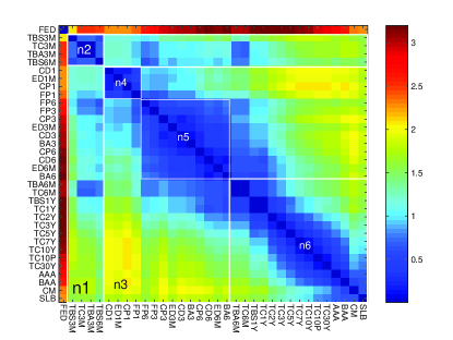
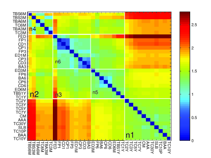
Figure 2: Left: Correlation heat map for the USIR dataset. Rectangles represent the classification yielded by the SPC technique. The general pattern is comparable with figure 3b on [20]. Right: Cointegration heat map for the USIR dataset with SPC classification again represented by rectangles. The general emergent pattern clusters short term Treasury instruments around $n4$, financial companies related instruments around $n3$ and long term instruments around $n1$.

There are several possible aims behind unsupervised segmentation based on a dissimilarity matrix $D$. Categorization from clustering algorithms has been used for market segmentation [10, 11]. For example, the Superparamagnetic Clustering (SPC) algorithm [12, 13] has been particularly useful since the number of clusters is not a priori known and the scale of resolution of the categories can be tuned by a temperature like parameter. Sometimes the data might not have a clear discrete class structure and here the SPIN algorithm provides a difference with its capability of helping identify low dimensional structures in a high dimensional space. Without knowing in advance what type of segmentation will emerge, the clustering and SPIN algorithms should be thought of as complementary. The aim of SPINing a similarity matrix is to obtain a permutation such that points close in distance are brought, by the permutation to places in the matrix that are also close. Since the space of permutations is factorially large this can easily be seen to be a potentially hard problem. The permutations are sequentially chosen, for example to minimize a cost function that penalizes large distances and puts them far from the diagonal or alternatively seek permutations that bring pairs with small distances near to the diagonal. Unless the structure can be ordered in one dimension, these requirements can lead to frustration. The class of cost functions proposed in [8] is of the form $\mathcal{F}(P)=$Tr$(PDP^{T}W)$, with $P$ being a permutation of matrix indices and $W$ a weight matrix which defines the algorithm. For their choices, namely, Side-to-Side (STS) defined as $W=XX^{T}$, with $X_{i}>X_{j}$ if $i>j$ and Neighborhood defined as $W_{ij}=exp(|i-j|\sigma)$, the minimization was shown to be NP-complete. The way out is to be satisfied with non optimal solutions that can be obtained in fast times ($\mathcal{O}(n^{2-3})$) and that turn out to be just as informative. The problem of sorting into categories is ill posed and therefore there will not be something like ‘the answer’. The reduction to an optimization problem, using either STS or Neighborhood leads to a NP-complete problem. It is fair to expect that any reasonable weight function will share that characteristic. So we have found that it is adequate to play around with the algorithms and apply them for different subsets, try optimizing the whole matrix, then choose a relevant cointegrating subset, optimize the subset, go up optimize the whole set, intercalate different algorithms. The result will tend to be better as measured by the cost function. This heuristics helps escape from local minima, of course it does not cure the fundamental problem that there might be frustration in a general sorting problem. This is not really a problem, good albeit not optimal solutions are just as informative as a perfect solution would be for all practical purposes. In the following analysis we have found that the best visualizations were simply achieved by employing the STS solution as an initial condition to the Neighborhood variant iterated with a schedule for reducing the scale parameter $\sigma$ in a simulated annealing fashion.

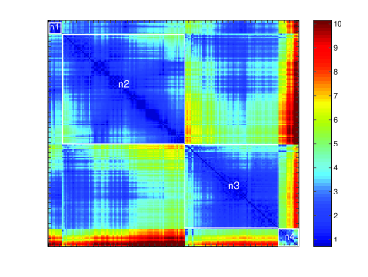
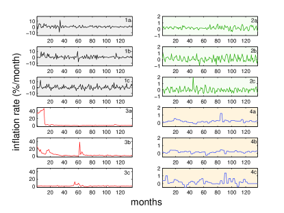
Figure 3: Left: SPINed cointegration map for the IFR dataset. The clusters that emerge correspond to economies with highly volatile prices (n1), developed economies with stable prices (n2), economies with events of hyperinflation in the period observed (n3) and economies with highly stable prices (n4). Right: Examples in each group. Group n1: Benin (1a), Central African Republic (1b) and Syria (1c). Group n2: USA (2a), Sweden (2b), Japan (2c). Group n3: Brazil (3a), Russia (3b) and Indonesia (3c). Group n4: Australia (4a), New Zealand (4b) and Tuvalu (4c).

4 Application examples

We exemplify the method by calculating cointegration maps for three data sets: (USIR) weekly US interest rates for 34 instruments from January 8, 1982 to August 29, 1997 ($T=817$ weeks) [14]; (IFR) monthly inflation rates for 179 countries from August, 1993 to December 2004 ($T=137$ months) [15]; (GDP) yearly gross domestic product growth rates for 71 countries from 1980 to 2004 ($T=25$ years) [16].

Measurement in soft sciences is itself a challenging activity [17]. Socio-economic systems are self-aware, there are severe limits to the accuracy of statistical data that can be gathered and even the definition of several macroeconomic quantities is still debatable [18, 19]. An exception to these data quality constraints are the organized financial markets like those of interest rate instruments in dataset USIR.

In figure 2 (left) we show the SPINed heat map for correlation coefficients of time series fluctuations. Pseudocolors are assigned according to dissimilarities calculated with eq. 16 by replacing the cointegration measure by correlation coefficients. In the same figure we show as rectangles identified by $n1,...,n6$ the hierarchical grouping structure generated by the SPC technique ($K=7$, see [12]). Characteristic of unsupervised classification techniques is the reliance of the results on the dissimilarity measure adopted. Despite the differences, the general patterns revealed in figure 2 compare well with those of figure 3b on [20], which employs a classical agglomerative clustering with a metric distance based on linear correlation coefficients. Notice that the SPINed heat map is capable of showing nuances in the relationship structure that are absent in the traditional or SPC approaches. For example, the Treasure bill rates with maturities 3 and 6 months (TBA3M and TBA6M) and other instruments of the same maturity, in particular, Treasure securities at constant maturity (TC3M and TC6M) correlate alike. However, this sort of information is lost both in the SPC classification and in [20] with the former classifying these instruments accordingly with their maturities and the latter grouping TBAs in one group and TCs in another.

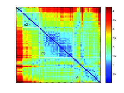
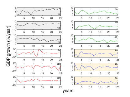
Figure 4: Left: SPINed cointegration map for the GDP dataset. The clusters that emerge correspond to countries with accelerating or decelerating economies (Group $n1$); developed countries with stable and accelerating economies (Group $n2$); volatile economies including major oil producers (Group $n3$) and stable economies (Group $n4$). Right: Examples in each group are. Group $n1$: Bangladesh (1a), Tanzania (1b) and Pakistan (1c). Groups $n2$: Norway (2a), United Kingdom (2b) and Japan (2c). Group $n3$: Kuwait (3a), Venezuela (3b) and Saudi Arabia (3c). Group $n4$: US (4a), Australia (4b) and Italy (4c).

Figure 2 (right) shows the cointegration map for USIR. Considering the reliability of the estimates ($\sigma_{\gamma}\approx 0.035$ for USIR), the map produced allows a direct visualization of relationships through the whole set of time series without imposing any ad hoc classification criteria. The classification provided by SPC ($K=7$) is also shown as rectangles identified by $n1,...,n6$. As we have already discussed, correlation of the fluctuations and cointegration are different relationship measures. Two time series will pertain to the same cointegration group if they tend to orbit a common time series. The general pattern groups short term Treasury bills in $n4$, long term instruments, both treasury and corporate around $n1$ and finance company related instruments (interbank eurodollar (EDs), certificates of deposit (CDs) and finance company papers (FPs)) around $n3$.

Figure 3 (left) shows the SPINed cointegration map for monthly inflation data (IFR). Even though the estimates are less reliable in this case ($\sigma_{\gamma}\approx 0.085$) it is possible to identify groups by inspecting their mutual relationships represented by the color map. Figure 3 (right) allows a direct interpretations of segmentation provided. Group $n1$ consists of countries that exhibit volatile inflation profiles with both high inflation and high deflation periods (Benin (1a), Central African Republic (1b) and Syria (1c)). Group $n2$ is mainly composed by advanced economies with stable inflation patterns (USA (2a), Sweden (2b) and Japan (2c)) and countries that are very closely related to them (e.g. Martinique, Singapore and Bahamas). Group $n3$ consists of countries that have experienced hyperinflation in the period observed (Brazil (3a), Russia (3b) and Indonesia (3c)). Group $n4$ contains countries with very stable and low inflation profiles, among them New Zealand (4b), that has adopted inflation targeting as early as 1988, Australia (4a), that also has adopted inflation targeting in 1993 and Tuvalu (4c) that adopts the Australian dollar as currency. However, apart from Australia and New Zealand, all the other countries that have adopted inflation targeting before the period observed (1993-2004) (Canada, Finland, Korea, Sweden and United Kingdom) have been classified in the Group $n2$.

The cointegration map for GDP data (Fig. 4 (left)) must be dealt with care as this data set is smaller ($T=25$) and, therefore, statistically less reliable than the previous two sets ($\sigma_{\gamma}\approx 0.2$). To minimize interpretation problems due to GDP measurement issues we have selected from the IMF database $71$ countries that have had market economies in the period observed (1980-2004). As a criterion to classify different groups, we have looked at general interaction patterns compatible with the limited reliability of the estimates. The SPINned matrix shows that there are four distinguishable classes, but that their boundaries are not sharp. This illustrates again the difference between SPIN and traditional clustering techniques. For the latter either sharp boundaries (e.g. for hierarchical and K-means techniques) or some sort of low dimensional structure (e.g. fuzzy clustering) must be imposed even when there are none [21]. We, therefore, have defined Group $n1$ as being composed by countries that interact with countries in Group $n2$. Group $n2$ consists of countries that interact with Group $n4$ and less strongly with Group $n3$. Group $n3$ is characterized by countries that do not interact with Group $n1$, interact strongly with Group $n4$ and less strongly with Group $n2$. Finally, Group $n4$ interacts with Groups $n2$ and $n3$ but not with Group $n1$. This procedure results in accelerating (Fig. 4 (right) Bangladesh (1a) and Tanzania (1b) ) or decelerating economies (Pakistan (1c)) in Group $n1$; low volatility economies both stable (Norway (2a) and United Kingdom (2b)) and decelerating (Japan (2c)) in Group $n2$; Group $n3$ concentrates highly volatile unstable economies including developing countries and all major oil producers (Kuwait (3a), Venezuela (3b) and Saudi Arabia (3c)); stable economies in Group $n4$ (US (4a), Australia (4b) and Italy (4c)). Notice that the difference between Groups $n4$ and $n2$ is their relation with Group $n1$, to say, the presence of some countries with accelerating or decelerating growth rates in $n2$.

5 Conclusion

In this paper we have developed a simple measure for long term pairwise relationships in sets of time series by introducing a Bayesian estimate for a cointegration distance. For visualization of the relationships, with a minimum introduction of ad hoc structures, we have borrowed from the repertoire of Bioinformatics the SPIN ordering technique to produce cointegration heat maps. We have exemplified the technique in three sets of time series of financial and economic interest and have been capable of identifying low-dimensional structures of economic sense emerging from the procedure.

Our aim in this work has been the development of tools that may be useful for discovering collective long term structures in economic time series. We think that a thorough understanding of the economic phenomena behind the observed patterns depends on our capability of describing the system interactions in some detail, what is out of the scope of the present work. Considering that socio-economic systems belong to a class of complex systems with unreliably known interactions and dynamics we regard pattern recognition tasks as hereby described a first important step towards a deeper quantitative understanding of such systems.

References

- [1] J.-P. Bouchaud, M. Potters, Theory of Financial Risk and Derivative Pricing, Cambridge University Press (2003).
- [2] R.F. Engle, C.W.J. Granger, Econometrica 55 (1987), 251-276.
- [3] J.G. Hamilton, Time Series Analysis, Princeton University Press (1994).
- [4] H. Hinrichsen, J. S. Weitz and E. Domany, J. Stat. Phys. 88, 617-636 (1997).
- [5] E.T. Jaynes, (G.L. Bretthorst ed.), Probability theory: the logic of science, Cambridge University Press (2003).
- [6] K. Hubrich, H. Lütkepohl, P. Saikkonen, Econometrics Reviews 20 3 (2001), 247-318.
- [7] G. Koop et al., Bayesian Approaches to Cointegration in Palgrave Handbook of Econometrics: Econometric Theory Volume 1 (K. Patterson ed.), Palgrave Macmillan (2006).
- [8] D. Tsafrir et al., Bioinformatics 21 102005 (2005), 2301-2308.
- [9] A.Y. Ng, M. I. Jordan, Y. Weiss, On Spectral Clustering: Analysis of an Algorithm, NIPS 2001.
- [10] T. Di Matteo et al., Physica A 355 (2005), 21-33.
- [11] M. Tumminello et al. PNAS 102 30 (2005) 10421-10426.
- [12] M. Blatt, S. Wiseman, E. Domany, Phys. Rev. Lett. 76 (1996) 3251-3254.
- [13] L. Kullmann, J. Kertész, R.N. Mantegna, Physica A 287 (2000), 412-419.
- [14] Available from http://www.federalreserve.gov.
- [15] Available from http://www.clevelandfed.org.
- [16] Available from http://www.imf.org.
- [17] M. Boumans, Measurement 38 (2005) 275-284.
- [18] N.R. Swanson, D. Van Dijk, Journal of Business and Economic Statistics 24(1) (2006) 24-42.
- [19] O. Morgenstern, On the Accuracy of Economic Observations, 2nd Ed., Princeton University Press (1991).
- [20] T. Di Matteo, T. Aste, R.N. Mantegna, Physica A 339 (2004), 181-188.
- [21] T. Hastie, R. Tibshirani, J.H. Friedman, The Elements of Statistical Learning, Springer (2003).