Multiscale coupling of molecular dynamics and hydrodynamics: application to DNA translocation through a nanopore

Abstract

We present a multiscale approach to the modeling of polymer dynamics in the presence of a fluid solvent. The approach combines Langevin Molecular Dynamics (MD) techniques with a mesoscopic Lattice-Boltzmann (LB) method for the solvent dynamics. A unique feature of the present approach is that hydrodynamic interactions between the solute macromolecule and the aqueous solvent are handled explicitly, and yet in a computationally tractable way due to the dual particle-field nature of the LB solver. The suitability of the present LB-MD multiscale approach is demonstrated for the problem of polymer fast translocation through a nanopore. We also provide an interpretation of our results in the context of DNA translocation through a nanopore, a problem that has attracted much theoretical and experimental attention recently.

1 Introduction

Mathematical modeling and computer simulation of biological systems is in a stage of burgeoning growth. Advances in computer technology but also, perhaps more importantly, breakthroughs in simulational methods are helping to reduce the gap between quantitative models and actual biological behavior. The main challenge remains the wide and disparate range of spatio-temporal scales involved in the dynamical evolution of complex biological systems. In response to this challenge, various strategies have been developed recently, which are in general referred to as “multiscale modeling”. Some representative examples include hybrid continuum-molecular dynamics algorithms [1], heterogeneous multiscale methods [2], and the so-called equation-free approach [3]. These methods combine different levels of the statistical description of matter (for instance, continuum and atomistic) into a composite computational scheme, in which information is exchanged through appropriate hand-shaking regions between the scales. Vital to the success of this information exchange procedure is a careful design of proper hand-shaking interfaces.

Kinetic theory lies naturally between the continuum and atomistic descriptions, and should therefore provide an ideal framework for the development of robust multiscale methodologies. However, until recently, this approach has been hindered by the fact that the central equation of kinetic theory, that is, the Boltzmann equation, was perceived as an equally demanding approach as molecular dynamics from the computational point of view, and of very limited use for dense fluids due to the lack of many-body correlations. As a result, multiscale modeling of nanoflows has developed mostly in the direction of the continuum/molecular dynamics paradigm [1].

Over the last decade and a half, major developments in lattice kinetic theory [4, 5] are changing the scene. Minimal forms of the Boltzmann equation can be designed on the lattice, which quantitatively describe the behavior of fluid flows in a way that is often computationally more advantageous than the continuum approach based on the Navier-Stokes equations. Moreover, lattice kinetic theory has proven capable of dealing with complex flows, such as flows with phase transitions and strong heterogeneities, for which continuum equations are exceedingly difficult to solve, if at all known (for a recent review see [6]). These advances have opened the road to developing new mesoscopic multiscale solvers [7]. The present work provides a successful implementation of such an approach. We will focus on the coupling of a mesoscopic fluid solver, the lattice Boltzmann method, with simulations at the atomistic scale employing explicit molecular dynamics. A unique feature of our approach is the dual nature of the mesoscopic kinetic solver, which propagates coarse-grained information (the single-particle Boltzmann probability distribution), along straight particle trajectories. This dual field/particle nature greatly facilitates the coupling between the mesoscopic fluid and the atomistic levels, both on conceptual and computational grounds.

The paper is organized as follows. In Section $\S$2 we present the basic elements of the multiscale methodology, namely the Lattice Boltzmann treatment of the fluid solvent, and its coupling to a Molecular Dynamics simulation of the solute biopolymer. In Section $\S$3, we present an application of this multiscale methodology to the problem of long polymer translocation through a nanopore; in particular, we analyze in detail the role of hydrodynamics in accelerating the translocation process. In Section $\S$4 we elaborate on the relevance of our results to the problem of DNA translocation, which has attracted much theoretical and experimental attention recently. We conclude in Section $\S$5 with general remarks and outlook for future extensions.

2 Lattice-Boltzmann - Molecular-Dynamics multiscale methodology

We consider the generic problem of tracing the dynamic evolution of a polymer molecule interacting with a fluid solvent. This involves the simultaneous interaction of several physical mechanisms, often acting on widely separate temporal and spatial scales. Essentially, these interactions can be classified in three distinct categories as solute-solute, solvent-solvent and solvent-solute. The first category includes the conservative many-body interactions among the single monomers in the polymer chain. Being atomistic in nature, these interactions usually set the shortest scale in the overall multiscale process. They are typically handled by Molecular Dynamics techniques for constrained molecules. The second category, the solvent-solvent interactions, refer to the dynamics of the solvent molecules, which are usually dealt with by a continuum fluid-mechanics approach; in the present work these will be described by the mesoscopic Lattice Boltzmann equation. The second and third category have also been handled by simulating the solvent explicitly via molecular dynamics, implicit solvent particles via Brownian dynamics including hydrodynamic interactions, or solving the corresponding Fokker-Planck equation [8]. Finally, the solvent-solute dynamics will be treated by augmenting the molecular dynamics side with dissipative fluid-molecule interactions (Langevin picture) and including the corresponding reaction terms in the fluid-kinetic equations.

2.1 Atomistic dynamics

We consider a polymer consisting of $N$ monomer units (also referred to as beads). The polymer is advanced in time according to the following set of Molecular Dynamics-Langevin equations for the bead positions $\vec{r}_{p}$ and velocities $\vec{v}_{p}$:

$$\frac{d\vec{r}_{p}}{dt} = \vec{v}_{p}$$ (1)

$$m\frac{d\vec{v}_{p}}{dt} = \vec{F_{p}}^{c}+\vec{F_{p}}^{f}+\vec{F_{p}}^{r}+\vec{F_{p}}^{\kappa},\;\,\,\,p=1,N$$ (2)

where we distinguish four types of forces:

$$\vec{F_{p}}^{c~{}} = -\sum_{q}\partial_{\vec{r}_{p}}V(\vec{r}_{p}-\vec{r}_{q})$$ (3)

$$\vec{F_{p}}^{f~{}} = \gamma(\vec{u}_{p}-\vec{v}_{p})$$ (4)

$$\vec{F_{p}}^{r~{}} = m\vec{\xi}_{p}$$ (5)

$$\vec{F_{p}}^{\kappa} = -\lambda_{p}\partial_{\vec{r}_{p}}\kappa_{p}$$ (6)

The first term represents the conservative bead-bead interactions through a potential which we will take to have the standard $6-12$ Lennard-Jones form,

$$V_{LJ}(r)=4\epsilon[(\sigma/r)^{12}-(\sigma/r)^{6}]$$ (7)

truncated at a distance of r=$2^{1/6}\sigma$ [9]. This was combined with a harmonic part to account for the energy cost of distorting the angular degrees of freedom,

$$V_{ang}(\phi)=\frac{\kappa\phi^{2}}{2}$$ (8)

with $\phi$ the relative angle between two consecutive bonds. Torsional motions will not be included in the present model, but can easily be incorporated if needed.

We consider next the solute-solvent interactions. The second term on the right-hand-side of Eq.(1) represents the mechanical friction between the single bead and the surrounding fluid, $\vec{v}_{p}$ being the bead velocity and $\vec{u}_{p}$ the fluid velocity evaluated at the bead position. In addition to mechanical drag, the polymer feels the effects of stochastic fluctuations of the fluid environment, through the random term, $\vec{\xi}_{p}$, a Gaussian noise obeying the fluctuation-dissipation relations:

$$<\vec{\xi}_{p}> = 0$$

$$<\vec{\xi}(\vec{r}_{p},t)\vec{\xi}(\vec{r}_{q},t^{\prime})> = \gamma(k_{B}T/m)V\delta(\vec{r}_{p}-\vec{r}_{q})\delta(t-t^{\prime})$$

where $V$ is the volume of the cell to which beads $p$ and $q$ belong. Finally, $\lambda_{p}\partial_{\vec{r}_{p}}\kappa_{p}$ is the reaction force resulting from $N-1$ holonomic constraints for molecules modelled with rigid covalent bonds:

$$\kappa_{p}\equiv|\vec{r}_{p+1}-\vec{r}_{p}|^{2}-r_{0}^{2}=0$$ (9)

$r_{0}$ being the prescribed bond length, and $\{\lambda_{p}\}$ is the set of $N-1$ Lagrange multipliers conjugated to each constraint. The usage of constraints instead of flexible bond lengths makes it possible to eliminate unimportant high-frequency intra-molecular motion which would render the underlying LB propagation prone to numerical instabilities. In this way, the time-step of the Molecular Dynamics part can be increased by about one order of magnitude, as much as the overall efficiency of the LBMD method, as we shall discuss in section $\S$2.5. Finally, in order to avoid spurious dissipation, the bead velocities are required to be strictly orthogonal to the relative displacements. Given the second order atomistic dynamics, the velocities must obey the independent constraints:

$$\frac{d\kappa_{p}}{dt}=(\vec{r}_{p+1}-\vec{r}_{p})\cdot(\vec{v}_{p+1}-\vec{v}_{p})=0$$ (10)

The constraints (9), (10) are enforced over positions and momenta separately via the SHAKE [10] and the RATTLE algorithms [11]. The implementation of these constraints requires the iterative solution of the system of equations (9)-(10), typically accomplished via standard Newton-Raphson techniques.

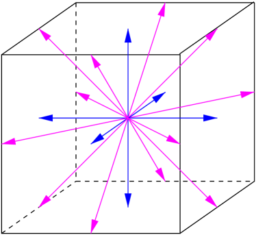
Fig. 1: The set of discrete speeds in the standard 19-speed 3D lattice for the Lattice-Boltzmann method.

2.2 Fluctuating Lattice Boltzmann method

The Lattice Boltzmann equation is a minimal form of the Boltzmann kinetic equation in which all details of molecular motion are removed except those that are strictly needed to recover hydrodynamic behavior at the macroscopic scale (mass-momentum and energy conservation). The result is an elegant equation for the discrete distribution function $f_{i}(\vec{x},t)$ describing the probability to find a particle at lattice site $\vec{x}$ at time $t$ with speed $\vec{v}=\vec{c}_{i}$. More specifically, since we are dealing with nanoscopic flows, in this work we shall consider the fluctuating Lattice Boltzmann equation which takes the following form:

$$f_{i}(\vec{x}+\vec{c}_{i}\Delta t,t+\Delta t)=f_{i}(\vec{x},t)-\omega\Delta t(f_{i}-f_{i}^{eq})(\vec{x},t)+F_{i}\Delta t+S_{i}\Delta t$$ (11)

where $f_{i}(\vec{x},t)$ represents the probability of finding a fluid particle at spatial location $\vec{x}$ and time $t$ with discrete speed $\vec{c}_{i}$. The particles can only move along the links of a regular lattice defined by the discrete speeds, so that the synchronous particle displacements $\Delta\vec{x}_{i}=\vec{c}_{i}\Delta t$ never take the fluid particles away from the lattice. For the present study, the standard three-dimensional 19-speed lattice is used [4] (see Figure 1). The right hand side represents the effect of intermolecular solvent-solvent collisions, through a relaxation toward local equilibrium, $f_{i}^{eq}$, typically a second order (low-Mach) expansion in the fluid velocity of a local Maxwellian with speed $\vec{u}$:

$$f_{i}^{eq}=w_{i}\rho\{1+\beta\vec{u}\cdot\vec{c}_{i}+\frac{\beta^{2}}{2}[\vec{u}\vec{u}:(\vec{c}_{i}\vec{c}_{i}-\beta^{-1}{\rm\vbox{\halign{#\cr$\leftrightarrow$\crcr \kern-1.0pt\nointerlineskip\cr$\hfil\displaystyle{I}\hfil$\crcr}}})]\}$$ (12)

where $\beta=m_{f}/k_{B}T_{f}$ is the inverse fluid temperature (with $k_{B}$ the Boltzmann constant), $w_{i}$ a set of weights normalized to unity, and I is the unit tensor in configuration space. The relaxation frequency $\omega$ controls the fluid kinematic viscosity $\nu$ through the relation:

$$\nu=c_{s}^{2}(1/\omega-\Delta t/2)$$ (13)

where $c_{s}$ is the sound speed in the solvent [7]. Knowledge of the discrete distributions $f_{i}$ allows the calculation of the local density $\rho$, flow speed $\rho\vec{u}$ and momentum-flux tensor $\leftrightarrow$ $\hfil\displaystyle{P}\hfil$ , by a direct summation upon all discrete distributions:

$$\rho(\vec{x},t) = \sum_{i}f_{i}(\vec{x},t)$$ (14)

$$\rho\vec{u}(\vec{x},t) = \sum_{i}f_{i}(\vec{x},t)\vec{c}_{i}$$ (15)

$$\vbox{\halign{#\cr$\leftrightarrow$\crcr \kern-1.0pt\nointerlineskip\cr$\hfil\displaystyle{P}\hfil$\crcr}}(\vec{x},t) = \sum_{i}f_{i}(\vec{x},t)\vec{c}_{i}\vec{c}_{i}$$ (18)

The diagonal component of the momentum-flux tensor gives the fluid pressure, while the off-diagonal terms give the shear-stress. Unlike in hydrodynamics, both quantities are available locally and at any point in the simulation.

Thermal fluctuations are included through the source term $F_{i}$ which reads as follows (index notation)

$$F_{i}=w_{i}\rho\{F^{(2)}_{ab}(c_{ia}c_{ib}-\beta^{-1}\delta_{ab})+F^{(3)}_{abc}g_{iabc}\}$$ (19)

where $F^{(2)}$ is the fluctuating stress tensor (a $3\times 3$ stochastic matrix). Consistency with the fluctuation-dissipation theorem at all scales requires the following conditions

$$\langle F^{(2)}_{ab}(\vec{x},t)F^{(2)}_{cd}(\vec{x}^{\prime},t^{\prime})\rangle={\gamma k_{B}T\over m}\Delta_{abcd}\delta(\vec{x}-\vec{x}^{\prime})\delta(t-t^{\prime})$$ (20)

where $\Delta_{abcd}$ is the fourth-order Kronecker symbol [12]. $F^{(3)}$ is related to the fluctuating heat flux and $g_{iabc}$ is the corresponding basis in kinetic space, essentially a third-order Hermite polynomial (full details are given in [13]).

The polymer-fluid back reaction is described through the source term $S_{i}$, which represents the momentum input per unit time due to the reaction of the polymer on the fluid population $f_{i}$:

$$S_{i}(\vec{x},t)=w_{i}\beta\sum_{p\in D(x)}[\vec{F}_{p}^{f}+\vec{F}_{p}^{r}]\cdot\vec{c}_{i}$$ (21)

where $D(x)$ denotes the mesh cell to which the p^th bead belongs. The quantities on the left hand side in the above expression have to reside on the lattice nodes, which means that the frictional and random forces need to be extrapolated from the particle to the grid location.

The use of a LB solver for the fluid solvent is particularly well suited to this problem because of the following reasons:
i) Free-streaming proceeds along straight trajectories. This is in stark contrast with hydrodynamics, in which fluid momentum is transported by its own space-time varying velocity field. Besides securing exact conservation of mass and momentum of the numerical scheme, this also greatly facilitates the imposition of geometrically complex boundary conditions.
ii) The pressure field is available locally, with no need of solving any (computationally expensive) Poisson problem for the pressure, like in standard hydrodynamics.
iii) Unlike hydrodynamics, diffusivity is not represented by a second-order differential operator, but it emerges instead from the first-order LB relaxation-propagation dynamics. The result is that the kinetic scheme can march in time-steps which scale linearly, rather than quadratically, with the mesh resolution. This facilitates high-resolution down-coupling to atomistic scales.
iv) Solute-solute interactions preserve their local nature since they are explicitly mediated by the solvent molecules through direct solvent-solute interactions. As a result, the computational cost of hydrodynamic interactions scales only linearly with the length of the polymer (no long-range interactions).
v) Since all interactions are local, the LB scheme is ideally suited to parallel computing.

It is worth mentioning that more advanced Lattice Boltzmann models [14, 15] could equally well be coupled to the atomistic dynamics.

2.3 Time exchange

The Molecular-Langevin-Dynamics solver is marched in time with a stochastic integrator (due to extra non-conservative and random terms), proceeding at a fraction of the LB time-step,

$$dt=\Delta t/M$$

The time-step ratio $M>1$ controls the scale separation between the solvent and solute timescales.

The numerical solution of the stochastic equations is performed by means of a modified version of the Langevin Impulse propagation scheme, derived from the assumption that the systematic forces are constant between consecutive time steps [16]. The propagation of the unconstrained dynamics proceeds according to the scheme [17]

$$~{}~{}~{}~{}~{}~{}~{}~{}~{}\tilde{r}_{p} = r_{p}(t)+\frac{dt}{2}v_{p}(t)$$

$$~{}~{}~{}~{}~{}~{}~{}~{}~{}v_{p}^{\star}(t+dt) = e^{-\gamma dt}\left\{v_{p}(t)+\left(\frac{e^{\gamma dt}-1}{\gamma m}\right)\left(F(\tilde{r}_{p})+\gamma u_{p}\right)+\left(e^{\gamma dt/2}+1\right)C(dt)\right\}$$

$$~{}~{}~{}~{}~{}~{}~{}~{}~{}r_{p}^{\star}(t+dt) = \tilde{r}_{p}+\frac{dt}{2}v_{p}(t+dt)$$ (22)

where $C(dt)$ is an array of $3N$ gaussian random variables with zero mean and variance $\frac{k_{B}T}{m}(e^{2\gamma dt}-1)$, and $\{\tilde{r}\}$ represent temporary positions. The propagator (22) is particularly suitable for our purposes since it is second order accurate in time and robust, that is, it reduces to the symplectic Verlet algorithm for $\gamma\rightarrow 0$. Moreover, at variance with the original Langevin Impulse scheme, the modified propagator allows for an unambiguous definition of velocities, which are needed to couple the polymer to the hydrodynamic field of the surrounding solvent. The particle positions and velocities corrected via the SHAKE and RATTLE algorithms read $\vec{r}^{\star}_{p}(t+dt)\rightarrow\vec{r}_{p}(t+dt)$ and $\vec{v}^{\star}_{p}(t+dt)\rightarrow\vec{v}_{p}(t+dt)$. For consistency, in considering the momentum exchange with the solvent the corrected velocities appear in the friction forces. The MD cycle is repeated $M$ times, with the hydrodynamic field frozen at time $t_{n}=n\Delta t$.

2.4 Spatial exchange

The transfer of spatial information from/to grid to/from particle locations is performed at each LB time-stamp $t_{n}=n\Delta t$. To this purpose,on account of its simplicity, a simple nearest grid point (NGP) interpolation scheme is used (see Fig.2). Momentum conservation was checked to hold up to six digits. With reference to a time slice $t_{n}=n\Delta t$, the pseudo-algorithm performing a single LB time-step, reads as follows

1. Interpolation of the velocity: $\vec{u}(\vec{x})\rightarrow\vec{u}_{p}$

2. For $m=1,M$:

   • Advance the molecular state from $t$ to $t+dt$

3. Extrapolation of the forces: $\vec{F_{p}}\rightarrow\vec{F}(\vec{x})$

4. Advance the Boltzmann populations from $t$ to $t+\Delta t$

This time-marching can be formally represented by an operator-splitting multi-step time procedure for two coupled kinetic equations describing the dynamic evolution for the fluid and the polymer distribution functions, respectively [18]. It is worth emphasizing that, while LB and MD with Langevin dynamics have been coupled before, notably in the study of single-polymer dynamics [19], to the best of our knowledge, this is the first time such that coupling is put in place for long molecules of biological interest.

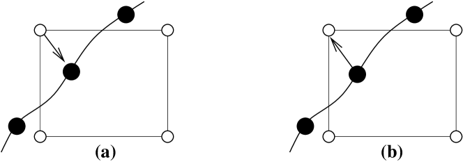
Fig. 2: Transfer of spatial information (a) from grid to particle, and (b) from particle to grid. Black spheres denote beads, while in white are the lattice sites.

2.5 Efficiency considerations

The total cost of the computation scales roughly like

$$t\sim(t_{LB}V+t_{MD}MN)N_{LB}$$ (23)

where $t_{LB}$ is the CPU time required to update a single LB site per timestep and $t_{MD}$ is the CPU time to update a single bead per timestep, $V$ is the volume of the computational domain in lattice units and $N$ is the number of polymer beads, with M the LB-MD time-step ratio. Finally, $N_{LB}$ is the number of LB timesteps. In the above equation, $t_{MD}$ includes the overhead of LB-MD coupling. Note that $t_{MD}$ is largely independent of $N$ because i) the LB-MD coupling is local, ii) the forces are short ranged and iii) the SHAKE/RATTLE algorithms are empirically known to scale linearly with the number of constraints.

Regarding the cost of the LB section, this is known to scale linearly with the volume occupied by the solvent. For the case where polymer concentration is kept constant, the volume needed to accommodate a polymer of $N$ beads should scale approximately as $N^{1.8}$; however, for translocation studies such as those discussed later in this paper, we shall consider a box of given volume, independently on the polymer length.

From the above expression it is clear that $M$ should be chosen as small as possible, consistent with the requirement of providing a realistic description of the polymer dynamics. In the present simulation we typically choose $M$ between $5$ and $20$, depending on the parameters of the simulation, particularly the temperature. This means that we are taking the LB representation close to the molecular scale. We will return to this important issue in the quantitative discussion of the physical application.

A tentative estimate of the computational cost proceeds as follows: Assuming $250$ flops/site/LB-step and $2500$ flops/bead/MD-step (including the LB-MD coupling overhead), and an effective processing speed of $100$ Mflop/s, the evolution over $30,000$ LB steps=$150,000$ MD steps of a typical $80\times 40\times 40$ grid and $400$ beads set-up, would take about:

$$t=30,000\times\big{[}250\times(80\times 40\times 4)+2500\times 5\times 400\big{]}/10^{8}=(9600+1500)sec\sim 3hrs,$$

which is in reasonable agreement with the simulation time observed with the present version of the code ($7hrs$), including the relative MD/LB cost ($\simeq 1:4$).

We wish to emphasize that the key feature of the LB-MD approach, namely linear scaling of the CPU cost with the number of beads (at constant volume) is indeed observed. In fact, the execution times for $50$, $100$ and $400$ beads are $0.433$, $0.489$, and $0.882$ sec/step, respectively on a 2GHz AMD Opteron processor. By excluding hydrodynamics, these numbers become $0.039$, $0.075$, and $0.318$ sec/step. It is worth mentioning that thus far, no effort has been directed to code optimization; it is quite possible that careful optimization may lower the execution time by an order of magnitude.

2.6 Validation tests

The static and dynamic behavior of the DNA chain obtained by our methodology has been compared to the scaling predictions for a single chain at infinite dilution. Given the structure factor $S_{f}(k)=\frac{1}{N}\sum_{i,j}\langle e^{ik\cdot(r_{i}-r_{j})}\rangle$, standard theory predicts the scaling law $S_{f}(k)=Ng(kR_{g})$, where $g(y)$ is a universal function and $R_{g}=(1/2N^{2})\sum_{i,j}\langle(r_{i}-r_{j})^{2}\rangle$ is the gyration radius. For large $k$, the structure factor is independent of $N$, and it follows

$$S_{f}(k)\propto k^{-1/\mu}$$

where experiments, theory and simulations agree on the scaling exponent value $\mu\simeq 0.584$. The static scaling law is not affected by the presence of hydrodynamics. However, verification of the scaling law and attainment of the scaling regime for large enough chains is a good check for the correctness of our simulation scheme and for the subsequent validation of the hydrodynamic behavior.

The dynamic behavior of the chain is deeply affected by the presence of hydrodynamic interactions. The standard picture of polymer dynamics is based on the Rouse (no hydrodynamics) or Zimm (hydrodynamic) description in terms of an underlying gaussian chain. In this case, the chain intermediate scattering function $I_{S}(k,t)=\frac{1}{NS_{f}(k)}\sum_{i,j}\langle e^{ik\cdot[r_{i}(t)-r_{j}(0)]}\rangle$ should follow the universal behavior

$$I_{S}(k,t)=\tilde{g}(D_{f}R_{g}^{x-2}tk^{x})$$

where $\tilde{g}(y)$ is another universal function and $D_{f}$ is the center of mass diffusion constant. Having introduced the dynamic scaling exponent $\mu^{\prime}$ via $D_{f}\sim N^{\mu^{\prime}}$, the exponent $x$ is found to be $x=2+\mu^{\prime}/\mu$. According to Zimm theory, $\mu^{\prime}=\mu$ and $x=3$ [19] while, according to Molecular Dynamics simulations, it appears that the actual value is somehow lower, i.e. $x\simeq 2.9$ [20].

We have considered a chain made of 30 monomers with bead-bead Lennard-Jones parameters taken from previous studies of chains simulated via Brownian dynamics [21] ($\sigma=0.65$, $\epsilon/k_{B}T=1.0$, bond length $r_{0}=0.945$) in a simulation box of edge $60$. This choice was motivated to verify the range of scaling behavior as compared to previous numerical results. We have computed the structure factor, as reported in Fig.3(a), and observed that the scaling regime is clearly visible for $1<k<3$ with an exponent equal $\mu=0.58\pm 0.1$. In the range of $k$ vectors where the static scaling holds, the dynamic scaling has been checked by considering, for given values of the computed scattering function, the loci of points $t(k,I_{S})=\tilde{g}^{-1}(I_{S})k^{-x}$ and by fitting via a power law curve (see ref. [20] for details). As illustrated in Fig.3(b), the resulting scaling exponent is found to be $x=2.9\pm 0.1$, in excellent agreement with the expected value and similar to previous simulation results on single polymers surrounded by a Lattice Boltzmann fluid [21]. Moreover, by applying a heuristic argument [20], we have verified that within the scaling regime, the finite size of the periodic box was not biasing the data.

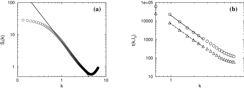
Fig. 3: (a) Log-log plot of the structure factor of a polymer in solution made of 30 monomers. The straight line is the power law fit in the range $1<k<3$ with exponent $\mu=0.58$. (b) Log-log parametric plot of $t(I_{S},k)$ vs $k$ for $I_{S}=0.3$ (circles) and $I_{S}=0.6$ (triangles). The lines represent the power law fits within the scaling region $1<k<3.0$ with exponent $x=2.9$.

3 Application: polymer translocation through nanopore

The scheme described above is general and applicable to any situation where a long polymer is moving in a solvent. This motion is of great interest for a fundamental understanding of polymer dynamics in the presence of the solvent. For example, the translocation of a polymer through a pore of very small size (of order the separation between monomers), is a process in which the coupling of the molecular motion to the solvent dynamics may be of crucial significance. In this section, we will therefore provide a detailed discussion of the polymer dynamics in the presence of a solvent for the example of translocation through a nanopore but without reference to a specific physical system. In the next section we explore the relevance of these results to DNA translocation through a nanopore.

3.1 Initial and Boundary conditions

The polymer is initialized via a standard self-avoiding random walk algorithm and further relaxed to equilibrium by standard Molecular Dynamics. The solvent is initialized with the equilibrium distribution corresponding to a constant density $\rho_{0}$ and zero macroscopic speed $\vec{u}=0$.

Boundary conditions for the fluid are periodic at inlet/outlet sections, and zero-speed at rigid walls, using the standard bounce-back rule [4]. For the polymer, periodicity is again imposed at inlet/outlet, whereas the interaction with rigid walls is handled by a Lennard-Jones potential with specific wall-polymer parameters $\sigma_{wall}=1.5$ and $\epsilon_{wall}=10^{-3}$ in LB units. The connection between slip-flow at the wall and intermolecular solid-fluid interactions shall be the objects of future research.

3.2 Numerical set-up

We consider a three-dimensional box of size $N_{x}h\times N_{y}h\times N_{z}h$ lattice units, with $h$ the spacing between lattice points. We will take $N_{x}=2N_{y}$, $N_{y}=N_{z}$; the separating wall is located in the mid-section of the $x$ direction, at $x=hN_{x}/2$ with $N_{x}=80$. At $t=0$ the polymer resides entirely in the right chamber at $x>hN_{x}/2$. At the center of the separating wall, a square hole of side $d_{hole}=2h$ is opened, through which the polymer can translocate from one chamber to the other. Translocation is induced by a constant electric field which acts along the $x$ direction, and is confined in a rectangular channel of size $2h\times h\times h$ along the streamline ($x$ direction) and cross-flow ($y,z$ directions). The spatial coarse-graining is such that the presence of the solvent as well as electrostatic forces acting due to charges on the polymer are neglected altogether as being of secondary importance compared to hydrodynamics.

Here and throughout we work in lattice Boltzmann units, in which length and time are measured in units of the lattice spacing $h=\Delta x$ and time-step $\Delta t$, respectively. Mass is defined as $m=m_{LB}m_{sol}$. The dimensionless mass $m_{LB}$ used in the simulations is set to unity, which means that mass is measured in units of the solvent mass $m_{sol}$. This choice is not restrictive since the present approach is used to model incompressible flows in which density is a parameter which can be rescaled by any arbitrary factor. However, it is of some interest to estimate the number of solvent molecules represented by a single LB computational molecule, since the inverse of this number conveys a measure of the importance of statistical fluctuations at the scale of the lattice spacing $\Delta x$. Let $S_{N}$ be this number, which will be defined as $\frac{\rho_{sol}h^{3}}{\rho_{LB}m_{sol}}$, where $\rho_{LB}$ is the dimensionless density used in the LB simulations. In order for the Boltzmann probability distribution to make sense as a statistical observable, $N_{LB}>>1$. For typical values of $\rho_{sol}=1$ gr/cm³, $m_{sol}\sim 20$ amu, $\rho_{LB}=1$ (which correspond to water), and $h$ in the range $1-10^{2}$ nm, this yields $S_{N}\sim 10^{4}-10^{6}$. This shows that the neglect of many-body fluctuations inherent to the single-particle Boltzmann representation is still justified even at the nanoscopic scale of the lattice spacing.

We will focus here on the fast translocation regime, in which the translocation time $t_{X}$ is much smaller than the Zimm time, $t_{Z}$, i.e. the typical relaxation time of the polymer towards its native (minimum energy, maximum entropy) configuration. Under fast-translocation conditions, the many-body aspects of the polymer dynamics cannot be ignored because different beads along the chain do not move independently. As a result, simple one-dimensional Brownian models do not apply [22]. In addition to many-body solute-solute interactions, the present approach also takes full account of many-body solute-solvent hydrodynamic interactions. The conditions for fast-translocation regime can be appraised as follows. The translocation time is estimated by equating the driving force, $F_{pull}$, to the drag force exerted by a solvent with dynamic viscosity $\eta$ on a polymer with radius of gyration $R$, $F_{drag}\sim\frac{6\pi\eta R^{2}}{t_{X}}$. This yields $t_{X}\sim\frac{6\pi\eta R^{2}}{F_{pull}}$. Since the Zimm time is given by $t_{Z}\sim\frac{0.4\eta R^{3}}{k_{B}T}$, the fast-translocation condition $t_{X}\ll t_{Z}$ becomes:

$$\frac{F_{pull}R}{k_{B}T}\gg\frac{6\pi}{0.4}\sim 50$$ (24)

Our reference simulation is performed with $F_{pull}/m=0.02\Delta x/\Delta t^{2}$ and $k_{B}T/m=10^{-4}\Delta x^{2}/\Delta t^{2}$, with $m$ the mass of one bead (monomer) of the polymer. The polymer length is in the range $20\leq N\leq 400$ beads. It can be readily checked that by assuming $R\sim N^{0.6}$ our set of parameters falls safely within the fast translocation regime. However, for $k_{B}T/m=10^{-3}$, $F_{pull}R/k_{B}T$ is of the order of $10^{2}-10^{3}$ which is much closer to breaking the above condition.

The main parameters of the simulation are (in LB units) $\sigma=1.8$ and $\epsilon=10^{-4}$ for the Lennard-Jones potential. The bond length among the beads is set at $r_{0}=1.2$. According to these values, the Lennard-Jones time-scale, $\tau_{LJ}=\sigma/\sqrt{2\epsilon/m}$, is of the order of $\sim 100\Delta t$. Thus, by choosing $M=5$ as a time-gap factor, we obtain $dt\sim\tau_{LJ}/500$, which is adequate for the resolution of the polymer dynamics. The solvent is set at a density $\rho=1$, with a kinematic viscosity $\nu=0.1\Delta x^{2}/\Delta t$ and a damping coefficient $\gamma=0.1/\Delta t$. The flexional rigidity $\kappa$ for the angular potential between beads will be $10^{-4}$/rad. In order to resolve the structure of the solvent accurately on the atomistic scale [23], we should use a higher resolution of at least 3-4 orders of magnitude. This means resolving the radial structure of the pore, a task that can only be undertaken by resorting to parallel computing. It is nonetheless hoped, and verified a posteriori, that this artificial magnification does not affect adversely the most significant dynamical and statistical properties of the translocation process, by which we mean that eventually, the time-scale of the simulated process may not be the same as in the physical process of interest, but the simulated dynamics is related to the physical dynamics by a simple rescaling of the time variable.

3.3 Translocation time

The most immediate quantity of interest in the translocation process is the dependence of the translocation time on the polymer length. This is usually expressed by a scaling law of the form

$$\tau_{X}(N)\equiv t_{x}/dt=N^{\alpha}$$

where $t_{0}$ is a reference time-scale, formally the translocation time of a single monomer, and $\alpha$ a scaling exponent measuring the degree of competition ($\alpha>1$) / cooperation ($\alpha<1$) of the various monomers in the chain.

We first turn to the derivation of the scaling behavior of the translocation process in the case where hydrodynamic interactions are included. In order to take into account the statistical nature of the phenomenon, simulations of a large number of translocation events ($100$ up to $1000$) for each polymer length were carried out. The ensemble of simulations is generated by different realizations of the initial polymer configuration. The duration histograms were constructed by cumulating all events for various lengths. Overall, our results are quite similar to the corresponding experimental data for DNA translocation through a nanopore [24], which we discuss in more detail in the following section.

At a next step, our data were shifted and scaled so that the distribution curve starts at zero-time and the total probability is equal to unity. The resulting distributions are on average not gaussians, but skewed towards long translocation times, consistent with experiment [24]. Therefore, the translocation time for each length is not assigned to the mean time, but to the most probable time, which is the position of the maximum in the histogram. In Fig.4 the distribution of all the events for polymer sizes N=50, 100 and 300 are shown. In this figure, the most probable translocation time for each length is denoted by an arrow. From this analysis, a nonlinear relation between the most probable translocation time $\tau_{0}$ and the polymer length is obtained that follows closely the theoretically expected scaling $\tau_{X}(N)\sim N^{\alpha}$, with $\alpha\sim 1.29$ (see Fig.4).

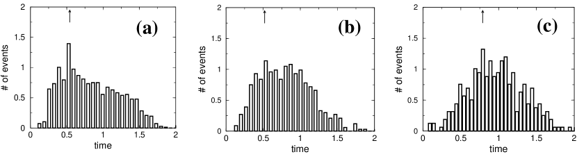
Fig. 4: Probability distributions of the translocation times for various lengths: (a) N =50, (b) N=100, and (c) N=300, respectively. Both axes are scaled to produce normalized probability distributions. The arrows show the most probable translocation time for each length.

Fig. 5: Translocation time as a function of the number of monomers for the case with hydrodynamics. The straight line represents the power law with exponent $1.29$. Time is shown in units of the LB timestep $\Delta t$.

3.4 Dynamics with and without a solvent

A closer inspection into the polymer dynamics reveals some interesting features. The molecule shows a blob-like conformation on either side of the membrane as it moves through the hole. It may either translocate very fast or move from one chamber to the other intermittently, with pauses. Both types of events are present with and without a fluid solvent. In addition, a careful analysis of all the translocated chains unravels the difference between slower and faster translocation within the same fast translocation regime. The nature of the variations in time is connected to the random fluctuations of the polymer throughout its motion, rather than the temperature or its length. These fluctuations are correlated to the entropic forces (gradient of the free energy with respect to a conformational order parameter, typically the fraction of translocated beads, see $r(t)$ below) acting on both translocated and untranslocated parts of the polymer. In fact, when a solvent is present, the interplay between these forces and $F_{drag}$, $F_{pull}$ determines the motion and the shape of the chain and thereby the translocation time. At some point part of the chain shapes up in an almost linear conformation increasing in this way the entropic force acting on it. This eventually leads to deceleration of the whole chain. Fig.6 shows an illustration of this argument, where a polymer chain, surrounded by a solvent is represented at a time where it starts to slow down. In this figure, a polymer with the same length but different initial configuration is also shown at the same time.

It is very instructive to monitor the progress in time of the number of translocated monomers $N(t)$. Note that $r(t)\equiv N(t)/N$ serves as a reaction-coordinate, with the translocation time defined by the condition $r(t_{X})=1$. The translocated monomers for processes with and without hydrodynamics are shown in Fig.7. For the former, events related to the polymers of Fig.6 are shown (curves $A_{1}$, $A_{3}$), as well as that related to the most probable time ($A_{2}$). The arrow in this figure indicates the timestep corresponding to the snapshots in Fig.6. The translocation for a given polymer proceeds along a curve virtually related to its initial configuration and its interactions with the fluid. It is clearly visible that there is no general trend. The non-hydrodynamic case is in principle different, especially in terms of the time range which is larger. This reveals the importance of hydrodynamic coherence.

Additional insight into the dynamics is obtained by altering the parameter set. This has not yet been extensively explored, but it was found that a choice of $k_{B}T=10^{-5}$, $F_{pull}=0.01$, and $\epsilon=0.002$ leads to the frequent retraction of the polymer. In other words, after having translocated a large fraction of its length, the polymer occasionally reverses its motion and anti-translocates away from the hole, never to find its way back into it. Moreover, we find that a polymer that retracted in the presence of a solvent, manages to fully translocate if the solvent is absent. It is interesting to observe that, in principle, no such type of anti-translocating behavior has been observed for short polymers. This indicates that hydrodynamics significantly speed-up and alter the nature of translocation, especially for long polymers at low temperatures. This highly irregular dynamics escapes any scaling or statistical analysis, as well as dynamic Monte Carlo simulations [25], and can only be revealed by self-consistent many-body hydro-dynamic simulations.

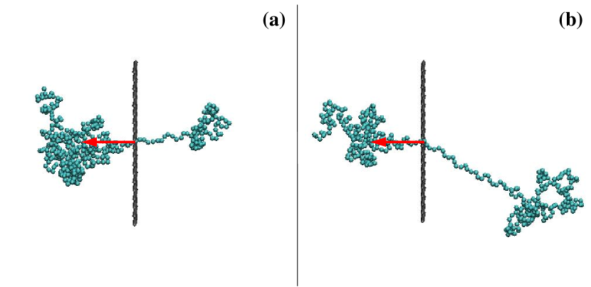
Fig. 6: Polymer configuration ($N=400$) corresponding to (a) fast and (b) slow translocation events. Both snapshots are shown at a timestep where the polymer (b) starts to slow down (see arrow in Fig.7). $F_{pull}$ is applied at the hole region towards a direction indicated by the arrow.

Fig. 7: Progress in time of the number of translocated beads for chains with $N=400$ monomers. Curves $A_{1}$, $A_{3}$ correspond to slow and fast translocation events (polymers shown in Fig.5), while $A_{2}$ to an event related to the most probable time. The initial configuration for the polymer in the event $B$ is the same as for $A_{2}$, but in that case no hydrodynamic interactions are included. Time is scaled with respect to the value of $\tau_{0}$ in the case with hydrodynamics. The arrow indicates the timestep at which the snapshots in Fig.6 are shown.

4 DNA translocation through a nanopore

The translocation of biopolymers, such as DNA and RNA plays a major role in many important biological processes, such as viral infection by phages, inter-bacterial DNA transduction, and gene therapy [26]. The importance of this process has spawned a number of in vitro experiments, aimed at exploring the translocation process through micro-fabricated channels under the effects of an external electric field, or through protein channels across cellular membranes [27]. In particular, recent experimental work has focused on the possibility of fast DNA-sequencing by reading the base sequence as the polymer passes through a nanopore. Some universal features of DNA translocation can be analyzed by means of suitably simplified statistical schemes [28] and non-hydrodynamic coarse-grained or microscopic models [29, 30]. However, a quantitative description of this complex phenomenon calls for state-of-the art modeling of the type described above. Accordingly, we explore here to what extent the results discussed above for the generic situation of polymer translocation apply to the DNA case.

First, we note that, as already mentioned in the previous section, our results are quite similar to the experimental data for DNA translocation through a nanopore [24]. Three different interpretations of the current model are physically plausible:
(a) Following the framework used in recent studies of DNA packing in bacteriophages [31], one monomer in our simulation can be thought of as representing a DNA segment of about 8 base-pairs, that is, each bead has a diameter of 2.5 nm, the hydrated diameter of B-DNA in physiological conditions.
(b) It is also physically plausible to assume that a bead represents a portion of DNA equivalent to its persistence length of about 50 nm, which translates into mapping one bead to $\sim$150 base-pairs.
(c) Alternatively, as is typically done in simulations of the $\lambda$-phage DNA in solution [32], one bead can be taken to correspond to $\sim 10^{3}$ base-pairs.
In all three cases $h=\Delta x$ is equal to the bead size, while the pore, having a width of 2$\Delta x$, will be different from the pores used experimentally, either smaller or larger. In addition, the coarse graining model that handles the DNA molecules indicates that the MD timescale is stretched over the physical process. A direct comparison between our probability distributions for polymer translocation and the experimental results sets a different MD timestep for the cases (a), (b), and (c) which is of the order of 3 nsec, 100 nsec and 5 $\mu$sec, respectively, leading to a LB timestep $\Delta t=5dt$ of 15 nsec, 500 nsec, and 25 $\mu$sec. It is difficult at this stage to assign a unique interpretation of our model in relation to a physical system. A thorough exploration of the parameter space is required before such an assignment can be made convincingly. This is beyond the scope of the present work but will be reported in future publications.

Fig. 8: Translocated ($R_{T}$), untranslocated ($R_{U}$) and effective ($R_{E}$) radii of gyration for the (a) non-hydrodynamic and (b) hydrodynamic cases with $N=400$. All radii are normalized with respect to the initial value $R_{U}(t=0)$. Time is also scaled with respect to the total translocation time $t_{X}$ for each of the events (a) and (b). The dotted lines denote the regions where $R_{E}$ is nearly constant (see text).

A second encouraging comparison is that the scaling we found for the translocation time with polymer length (with exponent $\alpha=1.29$) is quite close to the experimental measurement for DNA translocation [24] ($\alpha=1.27\pm 0.03$). Beyond the apparent consistency between experiment and theory, additional insight can be gained by analyzing the polymer dynamics during translocation.

A hydrodynamic picture of DNA translocation has been presented in ref. [24]. In this work, the authors assume that the electric field drive is in balance with the Stokes drag exerted by the solvent on the blob configuration of the polymer, that is

$$F_{pull}=6\pi\rho\nu{dR_{U}^{2}\over\tau}$$

where $\rho$ is the density, $\nu$ the kinematic viscocity, $\tau$ the translocation time, and $R_{U}$ the translocated part of the radius of gyration. In order for this balance to apply at all times, it is clear that $R^{2}$ must be constant in time, hence it cannot be identified neither with the translocated nor with the untraslocated gyration radius of DNA. To this end, in Fig.8 we represent the time-evolution of the radii of gyration for the two sections of DNA, $R_{U}(t)$ and $R_{T}(t)$, the untranslocated ($U$) [with $x>hN_{x}/2$] and translocated $(T)$ [with $x<hN_{x}/2$] parts, respectively. In order to identify a time-invariant radius, we define the $R_{I}(t)=QN_{I}^{\zeta}(t)$, where $I=U,T$ stands for the untranslocated and translocated parts and $N_{I}(t)$ is the corresponding number of monomers. The exponent $\zeta\sim 0.6$ is the same as previously noted and $Q$ is a constant (for long enough polymers). If translocation could be described by the dynamics of a single-blob object, characterized by an effective radius of gyration, defined as

$$R_{E}(t)=cN^{\zeta}(t),$$

then this quantity should be constant in time. Since the $N=N_{T}(t)+N_{U}(t)$ holds for all $t$, the above relations lead to

$$R_{E}(t)=[R_{T}^{1/\zeta}(t)+R_{U}^{1/\zeta}(t)]^{\zeta}=const$$ (25)

We focus first on the case without hydrodynamics, Fig.8(a). For very small chains $R_{I}(t)$ does not scale as $N_{I}^{0.6}$ and the definition for $R_{E}$ is not valid at the first and last $\sim 15-20\%$ parts of the event, during which the untranslocated and the translocated parts, respectively, are small. Outside these limits, $R_{E}(t)$ as obtained from the definition (25), with the values of $R_{U}(t),R_{T}(t)$ directly taken from the simulations, is indeed approximately constant. In addition, the values $R_{T}(t=t_{X})$ and $R_{U}(t=0)$ do not coincide, since the former is lower than the latter. This is also the case when a solvent is present, Fig.8(b). Thus, regardless of the dynamic pathway and the different conformations the chain may possess during translocation, once the event is completed the polymer is more compact than at $t=0$. Comparison of the cases with and without hydrodynamics reveals that in the latter case the polymer becomes up to $\sim 7\%$ more confined than when a solvent is added. The untranslocated part of the radius of gyration at the end of the process shows an abrupt drop. As a consequence the polymer $t=t_{X}$ does not fully recover its initial volume. It it plausible, that by allowing the polymer to further advance in time, $R_{T}(t=t_{X})$ will become similar to $R_{U}(t=t_{0})$, but this remains to be examined. Nevertheless, in this work we have been interested mainly on the chain dynamics related to the first passage times, which correspond to the exact period of time needed until all the beads have translocated.

5 Conclusions

We have presented a multiscale methodology based on the concurrent coupling of constrained molecular dynamics for the solute biopolymers with a lattice Boltzmann treatment of solvent dynamics. Owing to the dual field-particle nature of the Lattice Boltzmann technique, this coupling proceeds seamlessy in time and only requires standard interpolation/extrapolation for information-transfer in physical space. This multiscale methodology has been applied to the case of polymer translocation through a nanopore, with special emphasis on the role of hydrodynamic coherence on the dynamic and statistical properties of the translocation process. It is found that hydrodynamic interactions play a major role in accelerating the translocation process, especially for long molecules at low temperature.

An attempt to connect these results to the process of DNA translocation through a nanopore revealed certain similarities with experiment, especially in the scaling law of the translocation time with polymer length. The presence of hydrodynamic interactions lead to a decrease in the translocation times, compared to the cases without a fluid solvent. Inspection of the variation of the translocated beads and the radii of gyration with time reveals interesting aspects of the DNA dynamics during translocation.

Future directions for the simulations include the detailed study of the effects of temperature, finite-length and geometrical details of the nanopore geometry, as well as electrostatic interactions of the DNA molecule with the surrounding fluid. To this end, resort to parallel computing is mandatory, and we expect the favourable properties of LB towards parallel implementations to greatly facilitate the task. Work along these lines is currently in progress.

Acknowledgements The authors wish to thank C. Pierleoni for valuable discussions and help with the validation tests.

References

- [1] N. G. Hadjiconstantinou and A. T. Patera, Heterogeneous atomistic-continuum representations for dense fluid systems, Int. J. Mod. Phys. C, 8 (1997), pp. 967–976; A. Wagner, E. Flekkoy, J. Feder, and T. Jossanq, Coupling molecular dynamics and continuum dynamics, Comp. Phys. Comm., 147 (2002), pp. 670–673; X. Nie, S. Y. Chen and W. E, A continuum and molecular dynamics hybrid method for micro- and nano-fluid flow, J. Fluid Mech., 500 (2004), pp. 55–64.
- [2] W. E, B. Engquist, Z. Y. Huang, Heterogeneous multiscale method: A general methodology for multiscale modeling, Phys. Rev. B, 67 (2003), 092101.
- [3] C. Theodoropoulos, Y. H. Qian and I. Kevrekidis, ”Coarse” stability and bifurcation analysis using time-steppers: A reaction-diffusion example, PNAS, 97 (2000), pp.9840–9843.
- [4] R. Benzi, S. Succi, and M. Vergassola, The lattice Boltzmann-equation - Theory and applications, Phys. Rep., 222 (1992), pp. 145–197; D. A. Wolf-Gladrow, Lattice gas cellular automata and lattice Boltzmann models, Springer-Verlag, New York 2000; S. Succi, The lattice Boltzmann equation, Oxford University Press, Oxford 2001.
- [5] G. Mc Namara, G. Zanetti, Use of the Boltzmann-equation to simulate lattice-gas automata, Phys. Rev. Lett., 61 (1988), pp. 2332–2335; F. Higuera, S. Succi, and R. Benzi, Lattice gas-dynamics with enhanced collisions, Europhys. Lett., 9 (1989), pp. 345–349; F. Higuera, J. Jimenez, Boltzmann approach to lattice gas simulations, Europhys. Lett., 9 (1989), pp. 663–668; H. Chen, S. Chen, W. Matthaeus, Recovery of the Navier-Stokes equations using a lattice-gas Boltzmann method, Phys Rev A, 45 (1992), pp. 5339–5342; Y. H. Qian, D. d’Humieres, P. Lallemand, Lattice BGK models for Navier-Stokes equation, Europhys. Lett., 17 (1992), pp. 479–484; I.V. Karlin, A. Ferrante, H.C. Öttinger, Perfect entropy functions of the Lattice Boltzmann method, Europhys. Lett., 47 (1999), 182.
- [6] Proceedings of Discrete Simulation in Fluid Dynamics 2005, edited by B. Boghosian, special issue, Physica A, 362 (2006).
- [7] S. Succi, O. Filippova, G. Smith and E. Kaxiras, Applying the lattice Boltzmann equation to multiscale fluid problems, Computing in Science and Engineering, 3 (2001), pp. 26–37.
- [8] Martin Krger, Simple models for complex nonequilibrium fluids, Phys. Rep., 390 (2004), pp. 453-551; Martin Krger, A. Alba-Prez, M. Laso, H. C. ttinger, Variance reduced Brownian simulation of a bead-spring chain under steady shear flow considering hydrodynamic interaction effects, J. Chem. Phys., 113 (2000), pp. 4767-4773.
- [9] J. D. Weeks, D. Chandler, and H. C. Andersen, Role of Repulsive Forces in Determining the Equilibrium Structure of Simple Liquids, J. Appl. Phys., 54 (1971), pp. 5237–5247.
- [10] J. P. Ryckaert, G. Ciccotti, and H. J. C. Berendsen, Numerical-integration of cartesian equations of motion of a system with constraints - Molecular-Dynamics of n-alkanes, J. Comp. Phys. 23, (1977), pp.327–341.
- [11] H. C. Andersen, Rattle - A velocity version of the SHAKE algorithm for Molecular-Dynamics calsulations, J. Comput. Phys., 52 (1983), 24–34.
- [12] A. J. C. Ladd and R. Verberg, Lattice-Boltzmann simulations of particle-fluid suspensions, J. Stat. Phys., 104 (2001), pp. 1191–1251.
- [13] R. Adhikari, K. Stratford, M. E.Cates and A.J. Wagner, Fluctuating Lattice Boltzmann, Europhys.Lett., 71 (2005), pp. 473–477.
- [14] S. Ansumali, I.V. Karlin and H.C. Höttinger, Minimal entropic kinetic models for hydrodynamics, Europhys. Lett. 63 (2003), pp.798-804.
- [15] S. Ansumali and I.V. Karlin, Consistent Lattice Boltzmann method, Phys. Rev. Lett. 95 (2005), art. no. 260605.
- [16] R. D. Skeel and J. A. Izaguirre, An impulse integrator for Langevin dynamics, Mol. Phys., 100 (2002), pp. 3885–3891.
- [17] S. Melchionna, in preparation.
- [18] M. Tuckerman, and B. Berne, Vibrational-relaxation in simple fluids - Comparison of theory and simulations, J. Chem. Phys., 98 (1993), pp. 7301–7318.
- [19] P. Ahlrichs and B. Duenweg, Lattice-Boltzmann simulation of polymer-solvent systems, Int. J. Mod. Phys. C, 9 (1999), pp. 1429–1438; Simulation of a single polymer chain in solution by combining lattice Boltzmann and molecular dynamics, J. Chem. Phys., 111, (1999) 8225–8239; A. Chatterji, J. Horbach, Combining molecular dynamics with Lattice Boltzmann: A hybrid method for the simulation of (charged) colloidal systems, J. Chem. Phys., 122(18), (2005), 184903.
- [20] M. Doi, S.F. Edwards, The theory of polymer dynamics, Clarendon, Oxford, 1986.
- [21] C. Pierleoni, J.-P. Ryckaert, Molecular dynamics investigation of dynamic scaling for dilute polymer solutions in good solvent conditions, J. Chem. Phys., 96 (1992), pp.8539–8551; Excluded volume effects on the structure of a linear polymer under shear flow, ibid., 113 (2000), pp.5545–5558.
- [22] Y. Kantor and M. Kardar, Anomalous dynamics of forced translocation, Phys. Rev. E, 69 (2004), 021806.
- [23] J. Horbach, S. Succi, Lattice Boltzmann versus Molecular Dynamics simulation of nano-hydrodynamic flows, Phys. Rev. Lett., 96 (2006), 224503.
- [24] A. J. Storm et al, Fast DNA translocation through a solid-state nanopore, Nanolett., 5 (2005), pp. 1193–1197.
- [25] S. S. Chern, A. E. Cadenas and R. D Colson, Three-dimensional dynamic Monte Carlo simulations of driven polymer transport through a hole in a wall, J. Chem. Phys., 115 (2001), pp. 7772–7782.
- [26] H. Lodish, D. Baltimore, A. Berk, S. Zipursky, P. Matsudaira, and J. Darnell, Molecular Cell Biology, W.H. Freeman and Company, New York, 1996.
- [27] J. J. Kasianowicz, E. Brandin, D. Branton, and D. W. Deamer,Characterization of individual polynucleotide molecules using a membrane channel, PNAS, 93, (1996), pp. 13770–13773; A. Meller, L. Nivon, E. Brandin, J. Golovchenko, and D. Branton, Rapid nanopore discrimination between single polynucleotide molecules, PNAS, 97 (2000), pp. 1079–1084.
- [28] W. Sung and P. J. Park, Polymer translocation through a pore in a membrane, Phys. Rev. Lett., 77 (1996), 783–786.
- [29] S. Matysiak, A. Montesi, M. Pasquali, A. B. Kolomeisky, and C. Clementi, Dynamics of polymer translocation through nanopores: Theory meets experiment, Phys. Rev. Lett., 96 (2006), 118103.
- [30] D. K. Lubensky and D. R. Nelson, Driven polymer translocation through a narrow pore, Biophys. J., 77 (1999), pp. 1824–1838.
- [31] A. J. Spakowitz and Z-G Wang, DNA packaging in bacteriophage: Is twist important?, Biophys. J., 88 (2005), pp. 3912–3923; C. Forrey and M. Muthukumar, , doi:10.1529/biophysj.105.073429 and references therein.
- [32] T. T. Perkins, D. E. Smith, S. Chu, Single polymer dynamics in an elongational flow, Science, 276 (1997), 2016–2021; J. S. Hur, E. S. G. Shaqfeh, and R. G. Larson, Brownian dynamics simulations of single DNA molecules in shear flow, J. Rheol., 44 (2000), pp. 713–742; R. M. Jendrejack, J. J. de Pablo, and M. D. Graham, Stochastic simulations of DNA in flow: Dynamics and the effects of hydrodynamic interactions, J. Chem. Phys., 116 (2002), 7752–7759.