Reversals in nature and the nature of reversals

$\dagger$Forschungszentrum Dresden-Rossendorf, P.O. Box 510119, D-01314 Dresden, Germany
$\ddagger$LICRYL - INFM/CNR, Ponte P. Bucci, Cubo 31C, 87036 Rende (CS), Italy

The asymmetric shape of reversals of the Earth’s magnetic field indicates a possible connection with relaxation oscillations as they were early discussed by van der Pol. A simple mean-field dynamo model with a spherically symmetric $\alpha$ coefficient is analysed with view on this similarity, and a comparison of the time series and the phase space trajectories with those of paleomagnetic measurements is carried out. For highly supercritical dynamos a very good agreement with the data is achieved. Deviations of numerical reversal sequences from Poisson statistics are analysed and compared with paleomagnetic data. The role of the inner core is discussed in a spectral theoretical context and arguments and numerical evidence is compiled that the growth of the inner core might be important for the long term changes of the reversal rate and the occurrence of superchrons.

Keywords: Dynamo; $\alpha$ effect; Earth’s magnetic field reversals; inner core; Poisson statistics

1 Introduction

It is well known from paleomagnetic measurements that the axial dipole component of the Earth’s magnetic field has reversed its polarity many times (Merrill et al. 1996). The last reversal occurred approximately 780000 years ago. Averaged over the last few million years the mean rate of reversals is approximately 5 per Myr. At least two superchrons have been identified as periods of some tens of million years containing no reversal at all. These are the Cretaceous superchron extending from approximately 118 to 83 Myr, and the Kiaman superchron extending approximately from 312 to 262 Myr. Only recently, the existence of a third superchron has been hypothesized for the time period between 480-460 Myr (Pavlov and Gallet 2005).

Apart from their irregular occurrence, one of the most intriguing features of reversals is the pronounced asymmetry in the sense that the decay of the dipole is much slower than the subsequent recreation of the dipole with opposite polarity (Valet and Meynadier 1993, Valet et al. 2005). Observational data also indicate a possible correlation of the field intensity with the interval between subsequent reversals (Cox 1968, Tarduno et al. 2001, Valet et al. 2005). A further hypothesis concerns the so-called bimodal distribution of the Earth’s virtual axial dipole moment (VADM) with two peaks at approximately 4 $\times$ 10²² Am² and at twice that value (Perrin and Shcherbakov 1997, Shcherbakov et al. 2002, Heller et al. 2003). There is an ongoing discussion about preferred paths of the virtual geomagnetic pole (VGP) (Gubbins and Love 1998), and about differences of the apparent duration of reversals when seen from sites at different latitudes (Clement 2004).

The reality of reversals is quite complex and there is little hope to understand all their details within a simple model. Of course, computer simulations of the geodynamo in general and of reversals in particular (Wicht and Olson 2004, Takahashi et al. 2005) have progressed much since the first fully coupled 3D simulations of a reversal by Glatzmaier and Roberts in 1995. However, the severe problem that simulations have to work in parameter regions (in particular for the magnetic Prandlt number and the Ekman number) which are far away from the real values of the Earth, will remain for a long time.

With view on these problems to carry out realistic geodynamo simulations, but also with a side view on the recent successful dynamo experiments (Gailitis et al. 2002), it is legitimate to ask what are the most essential ingredients for a dynamo to undergo reversals in a similar way as the geodynamo does.

Roughly speaking, there are two classes of simplified models which try to explain reversals (Fig. 1). The first one relies on the assumption that the dipole field is somehow rotated from a given orientation to the reversed one via some intermediate state (or states). The rationale behind this “rotation model” is that many kinematic dynamo simulations have revealed an approximate degeneration of the axial and the equatorial dipole (Gubbins et al. 2000, Aubert et al. 2004). A similar degeneration is also responsible for the appearance of hemispherical dynamos in dynamically coupled models (Grote and Busse 2000). In this case, both quadrupolar and dipolar components contribute nearly equal magnetic energy so that their contributions cancel in one hemisphere and add to each other in the opposite hemisphere.

The interplay between the nearly degenerated axial dipole, equatorial dipole, and quadrupole was used in a simple model to explain reversals and excursion in one common scheme (Melbourne et al. 2001). It is interesting that this model of non-linear interaction of the three modes provides excursion and reversals without the inclusion of noise.

A second model belonging to this class is the model developed by Hoyng and coworkers (Hoyng et al. 2001, Schmidt et al. 2001, Hoyng and Duistermaat 2004) which deals with one steady axial dipole mode coupled via noise to an oscillatory “overtone” mode. Again, the idea is that the magnetic energy is taken over in an intermediate time by this additional mode.

Figure 1: Two different principles to explain reversals in simple models.

Another tradition to explain reversals relies on the very specific interplay between a steady and an oscillatory branch of the dominant axial dipole mode. This idea was expressed by Yoshimura et al. (1984) and by a number of other authors (Weisshaar 1982, Sarson and Jones 1999, Phillips 1993, Gubbins and Gibbons 2002).

In a series of recent papers we have tried to exemplify this scenario within a strongly simplified mean-field dynamo model. The starting point was the observation (Stefani and Gerbeth 2003) that even simple $\alpha^{2}$ dynamos with a spherically symmetric helical turbulence parameter $\alpha$ can have oscillatory dipole solutions, at least for a certain variety of profiles $\alpha(r)$ characterized by a sign change along the radius. This restriction to spherically symmetric $\alpha$ models allows to decouple the axial dipole mode from all other modes which reduces drastically the numerical effort to solve the induction equation. Hence, the general idea that reversals have to do with transitions between the steady and the oscillatory branch of the same eigenmode could be studied in great detail and with long time series.

In (Stefani and Gerbeth 2005) it was shown that such a spherically symmetric dynamo model, complemented by a simple saturation model and subjected to noise, can exhibit some of the above mentioned reversal features. In particular, the model produced asymmetric reversals, a positive correlation of field strength and interval length, and a bimodal field distribution. All these features were attributable to the magnetic field dynamics in the vicinity of a branching point (or exceptional point) of the spectrum of the non-selfadjoint dynamo operator where two real eigenvalues coalesce and continue as a complex conjugated pair of eigenvalues. Usually, this exceptional point is associated with a nearby local maximum of the growth rate situated at a slightly lower magnetic Reynolds number. It is essential that the negative slope of the growth rate curve between this local maximum and the exceptional point makes even stationary dynamos vulnerable to noise. Then, the instantaneous eigenvalue is driven towards the exceptional point and beyond into the oscillatory branch where the sign change happens.

An evident weakness of this reversal model in the slightly supercritical regime was the apparent necessity to fine-tune the magnetic Reynolds number and/or the radial profile $\alpha(r)$ in order to adjust the dynamo operator spectrum in an appropriate way. However, in a follow-up paper (Stefani et al. 2006a), it was shown that this artificial fine-tuning becomes superfluous in the case of higher supercriticality of the dynamo (a similar effect was already found for disk dynamos by Meinel and Brandenburg (1990)). Numerical examples and physical arguments were compiled to show that, with increasing magnetic Reynolds number, there is a strong tendency for the exceptional point and the associated local maximum to move close to the zero growth rate line where the indicated reversal scenario can be actualized. Although exemplified again by the spherically symmetric $\alpha^{2}$ dynamo model, the main idea of this “self-tuning” mechanism of saturated dynamos into a reversal-prone state seems well transferable to other dynamos.

In another paper (Stefani et al. 2006b) we have compared time series of the dipole moment as they result from our simple model with the recently published time series of the last five reversals which occurred during the last 2 Myr (Valet et al. 2005). Both the relevant time scales and the typical asymmetric shape of the paleomagnetic reversal sequences were reproduced within our simple model. Note that this was achieved strictly on the basis of the molecular resistivity of the core material, without taking resort to any turbulent resistivity.

An important ingredient of this sort of reversal models, the sign change of $\alpha$ along the radius, was also utilized in the reversal model of Giesecke et al. (2005a). This model is much closer to reality since it includes the usual North-South asymmetry of $\alpha$. Interestingly, the sign change of $\alpha$ along the radius is by no means unphysical but results indeed from simulations of magneto-convection which were carried out by the same authors (Giesecke et al. 2005b).

It is one of the goals of the present paper to make a strong case for the “oscillation model” in contrast to the ”rotation model”. We will show that the asymmetry of the reversals is very well recovered by our model in the case of high (although not very high) supercriticality. At the same time, we will show that the “rotation model” in the version presented by Hoyng and Duistermaat (2004) leads to the wrong asymmetry of reversals.

We will start our argumentation by elucidating the intimate connection of reversals with relaxation oscillations as they are well known from the van der Pol oscillator (van der Pol 1926). Actually, the connection of dynamo solutions with relaxation oscillations had been discussed in the context of the 22 year cycle of Sun’s magnetic field (Mininni et al. 2000., Pontieri et al. 2003) and its similarity with reversals was brought to our attention by Clement Narteau (2005). We will provide evidence for a strong similarity of the dynamics of the van der Pol oscillator and of our simple dynamo model. We will also reveal the same relaxation oscillation character in the above mentioned reversals data.

In a second part we will discuss some statistical properties of our reversal model within the context of real reversal data. We will focus on the “clustering property” of reversals which was observed by Carbone et al. (2006) and further analyzed by Sorriso-Valvo et al. (2006).

A third focus of this paper will lay on the influence of the inner core on the reversal model. One of the usually adopted hypotheses on the role of the inner core goes back to Hollerbach and Jones (1993 and 1995) who claimed the conductivity of the inner core might prevent the magnetic field from more frequent reversals. We will discuss the core influence in terms of a particular spectral resonance phenomenon that was observed by Günther and Kirillov (2006). As a consequence, an increasing inner core can even favor reversals before it starts to produce more excursions than reversals. This will bring us finally to a speculation on the determining role the inner core growth might have on the long term reversal rate and on the (quasi-periodic?) occurrence of superchrons.

2 Reversals and relaxation oscillations

In this section, we will characterize the time series of simple mean field dynamos as a typical example of relaxation oscillations. In addition, we will delineate an alternative model which was proposed by Hoyng and Duistermaat (2004) as a toy model of reversals. The connection with real reversal sequences will be discussed in the last subsection.

2.1 The models

2.1.1 Van der Pol oscillator

The van der Pol equation is an ordinary differential equation of second order which describes self-sustaining oscillations. This equation was shown to arise in circuits containing vacuum tubes (van der Pol 1926) and relies on the fact that energy is fed into small oscillations and removed from large oscillations. It is given by

$$\frac{\partial^{2}y}{\partial t^{2}} = \mu(1-y^{2})\frac{\partial y}{\partial t}-y$$ (1)

which can be rewritten into an equivalent system of two coupled first order differential equations:

$$\frac{\partial y}{\partial t} = z$$ (2)

$$\frac{\partial z}{\partial t} = \mu(1-y^{2})z-y\;.$$ (3)

Evidently, the case $\mu=0$ yields harmonic oscillations while increasing $\mu$ provides increasing anharmonicity.

2.1.2 Spherically symmetric $\alpha^{2}$ dynamo model

For a better understanding of the reversal process we have decided to use a toy model which is simple enough to allow for simulations of very long time series (in order to do reasonable statistics), but which is also capable to capture distinctive features of hydromagnetic dynamos, in particular the typical non-trivial saturation mechanism via deformations of the dynamo source. Both requirements together are fulfilled by a mean-field dynamo model of $\alpha^{2}$ type with a supposed spherically symmetric, isotropic helical turbulence parameter $\alpha$ (Krause and Rädler 1980). Of course, we are well aware of the fact that a reasonable simulation of the Earth’s dynamo should at least account for the North-South asymmetry of $\alpha$ which is not respected in our model. Only in the last but one section we will discuss certain spectral features of such a more realistic model.

Starting from the induction equation for the magnetic field $\bf B$

$$\frac{\partial\bf{B}}{\partial t}={\bf\nabla\times(\alpha{\bf{B}})}+(\mu_{0}\sigma)^{-1}\nabla^{2}{\bf{B}}\;,$$ (4)

(with magnetic permeability $\mu_{0}$ and electrical conductivity $\sigma$) we decompose ${\bf{B}}$ into a poloidal and a toroidal component, according to ${\bf{B}}=-\nabla\times({\bf{r}}\times\nabla S)-{\bf{r}}\times\nabla T$. Then we expand the defining scalars $S$ and $T$ in spherical harmonics of degree $l$ and order $m$ with expansion coefficients $s_{l,m}(r,t)$ and $t_{l,m}(r,t)$. As long as we remain within the framework of a spherically symmetric and isotropic $\alpha^{2}$ dynamo problem, the induction equation decouples for each degree $l$ and order $m$ into the following pair of equations

$$\frac{\partial s_{l}}{\partial\tau} = \frac{1}{r}\frac{\partial^{2}}{\partial r^{2}}(rs_{l})-\frac{l(l+1)}{r^{2}}s_{l}+\alpha(r,\tau)t_{l}\;,$$ (5)

$$\frac{\partial t_{l}}{\partial\tau} = \frac{1}{r}\frac{\partial}{\partial r}\left(\frac{\partial}{\partial r}(rt_{l})-\alpha(r,\tau)\frac{\partial}{\partial r}(rs_{l})\right)-\frac{l(l+1)}{r^{2}}[t_{l}-\alpha(r,\tau)s_{l}]\;.$$ (6)

Since these equations are independent of the order $m$, we have skipped $m$ in the index of $s$ and $t$. The boundary conditions are $\partial s_{l}/\partial r|_{r=1}+{(l+1)}s_{l}(1)=t_{l}(1)=0$. In the following we consider only the dipole field with $l=1$.

We will focus on kinematic radial profiles $\alpha_{kin}(r)$ with a sign change along the radius which had been shown to exhibit oscillatory behaviour (Stefani and Gerbeth 2003). Saturation is enforced by assuming the kinematic profile $\alpha_{kin}(r)$ to be algebraically quenched by the magnetic field energy averaged over the angles which can be expressed in terms of $s_{l}(r,\tau)$ and $t_{l}(r,\tau)$. Note that this averaging over the angles represents a severe simplification since in reality (even for an assumed spherically symmetric kinematic $\alpha$) the energy dependent quenching would result in a breaking of the spherical symmetry.

In addition to this quenching, the $\alpha(r)$ profiles are perturbed by ”blobs” of noise which are considered constant within a correlation time $\tau_{corr}$. Physically, such a noise term can be understood as a consequence of changing boundary conditions for the flow in the outer core, but also as a substitute for the omitted influence of higher multipole modes on the dominant axial dipole mode.

In summary, the $\alpha(r,\tau)$ profile entering Eqs. (5) and (6) is written as

$$\alpha(r,\tau) = \frac{\alpha_{kin}(r)}{1+E^{-1}_{mag,0}\left[\frac{2s_{1}^{2}(r,\tau)}{r^{2}}+\frac{1}{r^{2}}\left(\frac{\partial(rs_{1}(r,\tau))}{\partial r}\right)^{2}+t_{1}^{2}(r,\tau)\right]}$$ (7)

$$+\xi_{1}(\tau)+\xi_{2}(\tau)\;r^{2}+\xi_{3}(\tau)\;r^{3}+\xi_{4}(\tau)\;r^{4}\;,$$

where the noise correlation is given by $\langle\xi_{i}(\tau)\xi_{j}(\tau+\tau_{1})\rangle=D^{2}(1-|\tau_{1}|/\tau_{corr})\Theta(1-|\tau_{1}|/\tau_{corr})\delta_{ij}$. In the following, $C$ will characterize the amplitude of $\alpha$, $D$ is the noise strength, and $E_{mag,0}$ is a constant measuring the mean magnetic field energy.

2.1.3 An alternative: The model of Hoyng and Duistermaat

Later we will compare our results with the results of the model introduced by Hoyng and Duistermaat (2004) which describes a steady axial dipole ($x$) coupled by multiplicative noise to a periodic “overtone” ($y+iz$). It is given by the ordinary differential equation system:

$$\partial_{t}x = (1-x^{2})x+V_{11}x+V_{12}y+V_{13}z$$ (8)

$$\partial_{t}y = -ay-cz+V_{21}x+V_{22}y+V_{23}z$$ (9)

$$\partial_{t}z = cy-az+V_{31}x+V_{32}y+V_{33}z\;.$$ (10)

Evidently, without noise terms $V_{ik}$ this systems decouples into a steady axial dipole and a periodic “overtone”.

2.2 Numerical results in the noise-free case

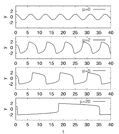
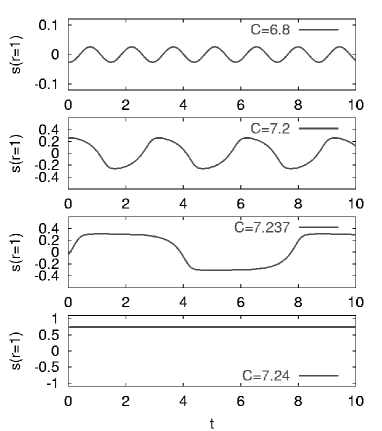
In Fig. 2 we show the numerical solutions of the van der Pol oscillator for different values of $\mu$, compared with the solutions of our dynamo model with a kinematic $\alpha$ profile according to $\alpha_{kin}(r)=1.916\cdot C\cdot(1-6\;r^{2}+5\;r^{4})$ (the factor 1.916 results simply from normalizing the radial average of $|\alpha(r)|$ to the corresponding value for constant $\alpha$). In the dynamo model we vary the dynamo number $C$ in the noise-free case (i.e. $D=0$). As already noticed, in the van der Pol oscillator we get a purely harmonic oscillation for $\mu=0$ which becomes more and more anharmonic for increasing $\mu$. A quite similar behaviour can be observed for the dynamo model. At $C=6.8$ (which is only slightly above the critical value $C_{c}=6.78$) we obtain a nearly harmonic oscillation which becomes also more and more anharmonic for increasing $C$. The difference to the van der Pol system is that at a certain value of $C$ the oscillation stops at all and is replaced by a steady solution ($C=7.24$).

Figure 2: Typical relaxation oscillations in the van der Pol model (left) and in the $\alpha^{2}$ dynamo model (right). With increasing $\mu$ and $C$, respectively, one observes an increasing degree of anharmonicity. In the dynamo case, this even goes over into a steady state.

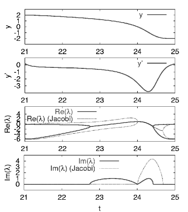
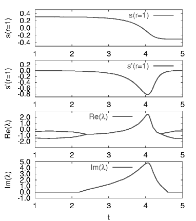
For the two values $\mu=2$ and $C=7.237$, respectively, we analyze the time evolution in more detail in Fig. 3. The upper two panels show $y(t)$ and $y^{\prime}(t)=z(t)$ in the van der Pol case and $s(r=1)$ and the time derivative $s^{\prime}(r=1)$ in the dynamo case. The lower two panels show the real and imaginary parts of the instantaneous eigenvalue $\lambda(t)$. A note is due here on the definition and the usefulness of such instantaneous eigenvalues. For the dynamo problem they result simply from inserting the instantaneous quenched $\alpha(r,t_{i})$ profiles at the instant $t_{i}$ into the time-independent eigenvalue equation. Quite formally, we could do the same for the van der Pol system by replacing in the nonlinear term in Eq. (3) $y^{2}$ by $y^{2}(t_{i})$. Of course, for a non-linear dynamical system it is more significant to consider the eigenvalues of the instantaneous Jacobi matrix which reads

$${\bf J}(y(t_{i}),z(t_{i}))=\left[\begin{array}[]{cc}0&1\\ -1-2\mu y(t_{i})z(t_{i})&\mu(1-y^{2}(t_{i}))\end{array}\right]$$ (13)

In the third and fourth line of the left panel of Fig. 3 we show the real and imaginary parts of this instantaneous Jacobi matrix eigenvalues, together with the eigenvalues resulting from the formal replacement of $y^{2}$ by $y^{2}(t_{i})$. It is not surprising that the latter shows a closer similarity to the instantaneous eigenvalues for the dynamo problem which are exhibited in the right panel.

Despite the slight differences, we see in any case that during the reversal there appears a certain interval characterized by a complex instantaneous eigenvalue which is “born” at an exceptional point where two real eigenvalues coalesce and which splits off again at a second exceptional point into two real eigenvalues.

Figure 3: Details and interpretation of the special cases $\mu=5$ and $C=7.237$ from Fig. 2, respectively. From top to bottom the panels show the main signal $y$ and $s(r=1)$, their time derivatives, and the real and imaginary parts of the instantaneous eigenvalues. In the van der Pol case, the latter are given in the correct version of the eigenvalue of the Jacobi matrix, and in the formal way which is also shown for the dynamo case.

It is also instructive to show the trajectories in the phase space, both for the van der Pol and for the dynamo problem. Figure 4 indicates that the systems are quite similar.

Figure 4: Phase space trajectories for the van der Pol oscillator and the dynamo with increasing $\mu$ and $C$, respectively.

2.3 Self-tuning into reversal prone states

Up to now we have only seen how a dynamo which is oscillatory in the kinematic and slightly supercritical regime changes, via increasingly anharmonic relaxation oscillation, into a steady dynamo for higher degrees of supercriticality. However, in the latter regime, we can learn much more when we analyze the spectrum of the dynamo operators belonging to the actual quenched $\alpha(r)$ profiles in the saturated state. This will help us to understand the disposition of the (apparently steady) dynamo to undergo reversals under the influence of noise.

For this purpose we have shown in Fig. 5 the growth rates (left) and the frequencies (right) of the dynamo in the (nearly) kinematic regime (for C=6.78) and for the quenched $\alpha$ profiles in the saturated regime with increasing values of $C$. Actually, the curves result from scaling the actual quenched $\alpha$ profiles with an artificial pre-factor $C^{*}$. This artificial scaling helps to identify the position of the actual eigenvalue (corresponding to $C^{*}=1$) relative to the exceptional point. For $C=6.78$, we see that the first and second eigenvalue merge at a value of $C^{*}$ at which the growth rate is less than zero. At $C^{*}=1$ it is evidently an oscillatory dynamo. However, already for $C=8$ the exceptional point has moved far above the zero growth rate line. Interestingly, for even higher values of $C$ the exceptional point and the nearby local maximum return close to the zero growth rate line. It can easily be anticipated that steady dynamos which are characterized by a stable fixed point become increasingly unstable with respect to noise. More examples of this self-tuning mechanism can be found in a preceding paper (Stefani et al 2006a).

Figure 5: Spectral properties of the nearly kinematic ($C=6.78$) and of the saturated $\alpha(r)$ profiles (for $C=$8, 10, 20, 50) which result from the chosen $\alpha_{kin}(r)=1.916\cdot C\cdot(1-6\;r^{2}+5\;r^{4})$. The scaling with the artificial factor $C^{*}$ helps to identify the actual eigenvalue (at $C^{*}=1$) in its relative position to the exceptional point. Note that for highly supercritical $C$ the exceptional point moves close to the zero growth rate line.

2.4 Reversals as noise induced relaxation oscillations

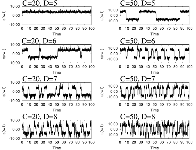
In this section, we will study highly supercritical dynamos under the influence of noise. We will vary the parameters $C$ and $D$ and check their influence on the time scale and the shape of reversals. Then we will compare the phase space trajectories during numerical reversals with those of paleomagnetic ones. Although the dynamo is not anymore in the oscillatory regime the typical features of relaxation oscillation re-appear during the reversal. Figure 6 shows typical magnetic field series for a time interval of 100 diffusion times which would correspond to approximately 20 Myr in time units of the real Earth. Not very surprisingly, the increase of noise leads to an increase of the reversal rate. The two documented values of $C$ indicate also a positive correlation of dynamo strength and reversal frequency, although this dependence is not always monotonic as was shown in (Stefani et al. 2006a).

Figure 6: Time series for various values of $C$ and $D$ for the kinematic profile $\alpha_{kin}(r)=1.916\cdot C\cdot(1-6\;r^{2}+5\;r^{4})$.

In Fig. 7 we compare now paleomagnetic time series during reversals with time series resulting form the $\alpha^{2}$ model on one side and from the Hoyng-Duistermaat model on the other side. Figure 7a represents the virtual axial dipole moments (VADM) during the last five reversals as they were published by Valet et al. (2005). Actually, the data points in Fig. 7a were extracted from Fig. 4 of (Valet et al. 2005). One can clearly see the strongly asymmetric shape of the curves with a slow dipole decay that takes around 50 kyr followed by fast dipole recovery taking approximately 5- 10 kyr. Since the curves represent an average over many site samples the VADM does not go exactly to zero at the reversal point. It is useful to take an average over these five curves in order to compare it with the time series following from various numerical models.

Figure 7: Comparison of paleomagnetic reversal data and numerically simulated ones. (a) Virtual axial dipole moment (VADM) during the 80 kyr preceeding and the 20 kyr following a polarity transition for five reversals from the last 2 million years (data extracted from (Valet et al. 2005)), and their average. (b) Five typical reversals resulting from the dynamo model with $\alpha_{kin}(r)=1.916\cdot C\cdot(1-6\;r^{2}+5\;r^{4})$ for $C=20$, $D=6$, and their average. (c) Five typical reversals resulting from the model of Hoyng and Duistermaat, and their average. Note that the time scale in this model has been chosen in such a way that it becomes comparable to geodynamo reversals. (d) Comparison of the average curves from (a), (c), and (b), complemented by two further examples with $C=8$, $D=1$ and $C=50$, $D=6$. The field scale for all the numerical curves has been fixed in such a way that the intensity in the non-reversing periods matches approximately the observed values.

The comparison of the real data with the numerical time series for $C=20$, $D=6$ in Fig. 7b shows a nice correspondence. Quite in contrast to this, the time series of the Hoyng-Duistermaat model show a wrong asymmetry (Fig. 7c). We compare the averages of real data, of our model results, and of the Hoyng-Duistermaat model results in Fig. 7d. Apart from the slightly supercritical case $C=8,D=1$ which exhibits a much to slow magnetic field evolution, the other examples with $C=$20, 50 and $D=6$ show very realistic time series with the typical slow decay and fast recreation. As noted above, the fast recreation results from the fact that in a small interval during the transition the dynamo operates with a nearly unquenched $\alpha(r)$ profile which yields, in case that the dynamo is strongly supercritical, very high growth rates.

With view on the relaxation oscillation property it may also be instructive to show the phase space trajectories in Fig. 8. In the curves of the real data, we have left out the data points very close to the sign change since these are not very reliable. Apart from this detail, we see in the paleomagnetic data and the numerical data the typical asymmetric shape of the phase space trajectories.

Figure 8: Phase space trajectories of real and numerical reversals. For the real data we have left out three points close to the very sign change position which are not very reliable.

3 Clustering properties of reversal sequences

The question whether the time intervals between reversals are governed by a Poisson process or not has been discussed by several authors (McFadden 1984, Constable 2000). The main difficulty in this approach is that, due to the poor statistics of the real data, the distribution of the time intervals between successive events is not clearly defined. In particular, it is not obvious to distinguish between an exponential distribution (that would be the case for a random, Poisson process) and a power-law process (indicating presence of correlations). Moreover, Constable (2000) has shown that the mean reversal rate is changing in the course of time, which would correspond to a non-stationary Poisson process with a time dependent rate function. This phenomenology could generate a power-law statistics for the inter-event times, even in absence of correlations. Only recently Carbone et al. (2006) were able to prove the non-Poissonian character of the reversal process by applying a criterion to the reversal sequence which works also for non-local Poisson processes.

Figure 9: The dependence $P(h>H)$ on $H$ for various numerical models and for the paleomagnetic date take from Cande and Kent (1995). For the parameter choice $C=20$, $D=6$ and $C=50$, $D=6$ we see a nearly perfect agreement with the real data. In contrast, the reversal data of the Hoyng model are much closer to a Poisson process.

A central quantity in their analysis is

$$H(\delta t,\Delta t) = 2\delta t/(2\delta t+\Delta t)$$ (14)

wherein, for a given reversal instant $t_{i}$, $\delta t$ is defined as the minimum of the preceding and subsequent time interval:

$$\delta t = \min\{t_{i+1}-t_{i};t_{i}-t_{i-1}\}\;.$$ (15)

$\Delta t$ is then the “pre-preceding” or ”sub-subsequent” time interval, respectively, according to

$$\Delta t = t_{i+2}-t_{i+1}\;\;\mbox{or}\;\;t_{i-1}-t_{i-2}\;.$$ (16)

The meaning of $H(\delta t,\Delta t)$ is quite simple: if reversals are clustered then the $\Delta t$ (which follows or precedes the $\delta t$ which is, by definition (10), assumed to be small) will also be small, and since $\Delta t$ appears in the denominator of Eq. (9), $H(\delta t,\Delta t)$ will be comparably large. In contrast, if the reversal sequence is governed by voids, then $\Delta t$ will be rather large and $H(\delta t,\Delta t)$ will be rather small. It can easily be shown that, for a sequence of random events, described by a Poisson process, the values of $H(\delta t,\Delta t)$ must be uniformly distributed in $[0,1]$. The interesting thing with this formulation is that, because of its local character, it indicates clustering or the appearance of voids even in the case of inhomogeneous Poisson processes (with time dependent rate function).

The sequence of paleomagnetic reversal data was shown to have a significant tendency to cluster (Carbone et al. 2006). In a follow-up paper (Sorriso-Valvo et al. 2006), various simplified dynamo models were examined with respect to their capability to describe this clustering process. In particular it turned out that the $\alpha^{2}$ dynamo model showed the right clustering property, although in a more pronounced way than the paleomagnetic data (Cande and Kent 1995).

In this section we analyze this behaviour a bit more in detail by checking the quantity H for a variety of values $C$ and $D$. In order to better emphasize and better visualize the shape of the $H$ distribution function, we show here the corresponding surviving function, namely the probability $P(h>H)$. In the Poisson (or local Poisson) case, that is uniform distribution of $H$, the surviving function would depend linearly on $h$, namely $P(h>H)=1-h$. The results are shown in Fig. 9. The dependence of $P(h>H)$ on H is shown for different values of $D$ from $C=20$ (Fig. 9a) and $C=100$ (Fig. 9b). In Fig. 9c, we compare the best curves for $C=20$, 50, and 100 with the paleomagnetic data (Cande and Kent 1995). Especially for $C=20$, $D=7$ and $C=50$, $D=6$ we observe a nearly perfect agreement, indicating that the temporal distribution of the reversals captures the real data features, including their tendency to cluster. In contrast to this, the model of Hoyng and Duistermaat shows more or less a Poisson behaviour (Fig. 9d). Note that the discrepancy of the results presented here for the Hoyng model from those reported in Carbone et al. (2006) and in Sorriso-Valvo et al. (2006), are due to the removal of the excursion-like events.

4 The role of the inner core

In this section we will study the influence of an inner core within the framework of our simple model. The usual picture of the role of the inner core was expressed in two papers by Hollerbach and Jones (1993, 1995). Basically, one expects that the conducting inner core impedes the occurrence of reversals by the effect that the magnetic field evolution is governed there by the long diffusion time scale and cannot follow the magnetic field evolution in the outer core which is governed by much shorter time scales of convection. Finally this will lead to a dominance of excursion over reversals (Gubbins 1999).

In the following we will check if and how this simple picture translates into our model. To begin with, we analyze the magnetic field evolution for a family of kinematic $\alpha$ profiles

$$\alpha_{kin}(x)=\frac{1.914\cdot C}{1+\exp{[(x_{0}-x)/d]}}\left[1.15-6\left(\frac{x-x_{0}}{1-x_{0}}\right)^{2}+5\left(\frac{x-x_{0}}{1-x_{0}}\right)^{4}\right]\;.$$ (17)

Basically this is a similar profile as considered before but the denominator $1+\exp{\left[(x_{0}-x)/d\right]}$ makes it vanishing in the inner core region with radius $x_{0}$ (including a smooth transition region of thickness $d$ which is simply used for numerical reasons).

Figure 10: The spectral explanation of excursions: Time evolution (a), instantaneous $\alpha(r)$ profiles (b), and instantaneous growth rates (c) for the kinematic $\alpha(x)$ according to Eq. (12) with special values $C=20$, $x_{0}=0.35$ and $d=0.05$.

For this model, with the special choice $C=20$, $x_{0}=0.35$ and $d=0.05$, Fig. 10a shows the time evolution of $s(x=1)$. In contrast to all models considered before, we get now an oscillation around a non-zero mean value (which was already observed by Hollerbach and Jones (1995)). Analogously as reversals can be traced to the transition between steady and oscillatory modes, the new “excursive” behaviour can also be explained in terms of the spectral properties of the underlying dynamo operator. To see this we consider in Fig. 10b the instantaneous $\alpha$ profiles at the instants 1, 2, 3, 4 indicated in Fig. 10a. For these instantaneous $\alpha$ profiles we show the first three eigenvalues in Fig. 10c, again in dependence on the artifical scaling parameter $C^{*}$. In this picture an excursion occurs as follows: First, at instant 1, the dominant eigenvalue is the complex one resulting from the merging of the second and third radial eigenmode. Its real part is clearly larger than the real part of the first eigenvalue. Being thus governed by a complex eigenvalue, the system starts to undergo a reversal. However, during this attempted oscillation the non-linear back-reaction becomes weaker (instant 2). Hence $\alpha$ becomes less quenched and we end up with a new instantaneous dynamo operator whose first real eigenvalue becomes dominant and whose second oscillatory branch becomes subdominant. Therefore, the system is governed now by a real and positive eigenvalue and the magnetic field increases again before it was able to complete the sign change. Later, the system returns to the state with stronger $\alpha$ quenching were the oscillatory mode becomes dominant again and so on.

That way, we have traced back excursions to the intricate ordering of the real first eigenvalue and the complex merger of the second and the third eigenvalue. The deep reason for this complicated behaviour has been indicated in the paper by Günther and Kirillov (2006), although for the case of zero boundary conditions which changes the spectrum drastically. In terms of the total $\alpha(r)$ profile, an inner core of a certain radius will contribute in form of higher radial harmonics. Splitting the induction equation into a coupled equation system for different radial harmonics (here Bessel functions) we observe a resonance phenomenon. Radial $\alpha$ profiles with higher harmonics in radial direction will also favour radial magnetic field modes with comparative wavelengths. Roughly speaking, an $\alpha(r)$ profile with one sign change along the radius (i.e. of the form $(1-6x^{2}+2-5x^{4})$) will favour the second eigenmode whose larger growth rate will tend to merge with that of the first eigenmode. Including a core, however, the third harmonic will be favoured and will merge with the second eigenfunction and so on.

Now let us switch to a core model with higher supercriticality. In Fig. 11 we considered the modified (and, admittedly, somewhat tuned) time dependent kinematic $\alpha(r)$ profile:

$$\alpha_{kin}(x) = \frac{1.914\cdot C}{1+\exp{\left[(x_{0}-x)/d\right]}}\times$$ (18)

$$\times\left[0.7+3\cdot x_{0}/1.914-6\left(\frac{x-x_{0}}{1-x_{0}}\right)^{2}+4.5\left(\frac{x-x_{0}}{1-x_{0}}\right)^{4}\right]$$

wherein the noise respects the core geometry in an appropriate manner

$$\Xi(r,\tau)=\frac{1}{1+\exp{\left[(x_{0}-x)/d\right]}}\left(\xi_{1}(\tau)+\xi_{2}(\tau)\;r^{2}+\xi_{3}(\tau)\;r^{3}+\xi_{4}(\tau)\;r^{4}\right)\;\;.$$ (19)

We carry out a simulation of this model, with $C=50$, $D=6$, and $d=0.05$, by increasing the inner core radius $x_{0}$ every 10 diffusion times by 0.05 (see Fig. 11b). The result can be seen in Fig. 11a.

Figure 11: The influence of a growing core on the reversal rate and the arising predominance of excursions.

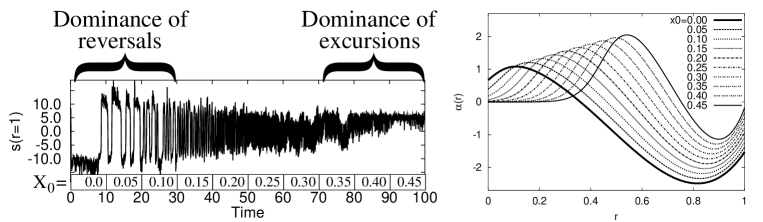
The first observation is that the role of the inner core is quite complicated. Starting from $x_{0}=0$ we see that with increasing $x_{0}$ the reversal frequency increases drastically. This is in clear contradiction to the Hollerbach and Jones picture. The second observation is that for larger $x_{0}$ the inner core indeed has a tendency to favour excursions in comparison with reversals which confirms again the Hollerbach and Jones view. At least we can see that the role of the inner core is much more complicated since the selection of modes which are coupling at an exceptional point depends very sensitively on its radius.

5 Towards more realistic models

We will conclude our study with an “excursion” into more realistic dynamo models. As we have seen, the time characteristics and the asymmetry of the real reversal process is well recovered within a simple dynamo model that requires only a dynamo operator with a local maximum of the growth rate and a nearby exceptional point where the two real eigenvalues merge and continue as oscillatory mode. This is a very unspecific requirement which does not rely on specific assumptions on the flow structure in the core. Nevertheless, it would be nice to see if and how this picture translates into more realistic dynamo models.

In the model of Giesecke (2005a), which includes the North-South asymmetry of $\alpha$ by virtue of a $\cos(\theta)$ term, quite similar reversal sequences were observed. Actually, in contrast to our model, Gieseckes model assumes a turbulent resistivity which is approximately 10 times larger than the molecular one. We believe that this necessity would disappear when going over from slightly to highly supercritical dynamos. In this respect it is instructive to compare again the two curves for $C=8$ and $C=20$ in Fig. 7d which are characterized by very different decay and growth times.

Apart from this detail, it is worthwhile to look a bit deeper into the spectral property of Gieseckes dynamo model. For that purpose we have analyzed the spectrum of the dynamo operator for functions of $\alpha(r,\theta)$ according to

$$\alpha_{kin}(r,\theta)=Rm\;\cos(\theta)\;\sin\left[2\pi(x-x_{0})/(1-x_{0})\right]\;.$$ (20)

Figure 12 shows the eigenvalues of the first five axisymmetric modes (m=0) and the first three non-axisymmetric modes (m=1) for different values of the inner core size $x_{0}$. The growth rates and frequencies result from an integral equation solver which was documented in previous papers (Stefani et al. 2000, Xu et al. 2004a, Xu et al. 2004b, Stefani et al. 2006c). The most important point which is changed by the inclusion of the $\cos(\theta)$ term is that now different $l$-modes are not independent anymore. Hence it may happen that modes with neighbouring $l$ merge at an exceptional point which was forbidden in the spherically symmetric model considered so far. Therefore, the scheme of mode coupling becomes even more complicated as before and one might expect a higher sensitivity with respect to changes of the inner core radius $x_{0}$.

Restricting our attention to the $m=0$ modes, we observe for $x_{0}=0$ an immediate coupling of the modes 2 and 3, which split off again close to $Rm=4$. The next coupling occurs close to $Rm=11.5$, but the resulting low lying mode seems not relevant for the reversal process. For $x_{0}=0.2$, the modes 2 and 3 are coupled from the very beginning, but the mode 1 and 4 couple also close to $Rm=13$. For $x_{0}=0.35$, which is approximately the case for the Earth, we see an immediate coupling of the modes 2 and 3 on one side and of the modes 4 and 5 on the other side. The latter split off again close to $Rm=16$, but shortly after this the mode 4 couples again with the mode 1. For $x_{0}=0.5$, the low modes show no coupling at all, only the mode 5 couples to the mode 6 which is, however, not shown in the plot.

Figure 12: Spectra for $\alpha^{2}$ dynamos respecting the North-South asymmetry by virtue of a $\cos(\theta)$ term, in dependence on the inner core size $x_{0}$.

In summary, this gives a complicated scheme of mode coupling and exceptional points which is quite sensitive to the value of $x_{0}$. What is missing at the moment is a detailed study of the spectral properties of the dynamo operator in the saturated regime which must be left to future work. We had indicated in Fig. 5 (and substantiated in more detail in (Stefani et al. 2006b)) that highly supercritical dynamos have a tendency to self-tune into a state in which they are prone to reversals. Hence Fig 12 can be quite misleading when it comes to the exact position of the exceptional points of the dominant mode. And, of course, one should not forget that the nearly degeneration between $m=0$ and $m=1$ will also be lifted if a tensor structure of $\alpha$ and further mean-field coefficients come into play as it is typical in more realistic mean-field models of the geodynamo (Schrinner et al. 2005, 2006).

6 Summary and speculations

We have checked the capability of a simple $\alpha^{2}$ dynamo model with spherical symmetric $\alpha$ to explain the typical time-scales and the asymmetric shape of Earth’s magnetic field reversals. The results are quite encouraging, in particular when comparing the paleomagnetic and the numerical reversal data in Figs. 7 and 8. In our view, the interpretation of reversals as noise induced relaxation oscillations seems quite natural. This mechanism of reversals relies on the existence of a local growth rate maximum and a nearby exceptional point of the spectrum of the dynamo operator in the saturated regime.

The clustering properties which were recently shown to be present in real paleomagnetic data (Carbone et al. 2006) were also observed in the model. Both the typical time scales of reversals and the degree of deviation from Poissonian statistics indicate that the Earth dynamo works in a regime of high, although not extremely high, supercriticality.

We conclude this paper with a speculation on a possible connection of the inner core radius with the long term behaviour of the reversal rate, including the occurrence of superchrons. It starts from the observation that the reversals rate of the last 160 Myr (see Merrill et al. 1996) suggests a time scale of long term variation in the order of 100 Myr. If one would take into account the Kiaman superchron, and possibly the (up to present unsettled) third superchron discovered by Pavlov and Gallet, one might hypothesize a process with a period of approximately 200 Myr. What could be the nature of such a periodicity (if there were any)? The first idea that comes to mind is the connection with slow mantle convection processes that influence, by virtue of changed core-mantle boundary conditions, the heat transport in the core, hence the dynamo strength and ultimately the reversal rate.

But what about the inner core? Is there a possibility that such a 200 Myr variability (or periodicity?) be related to a resonance phenomenon of the spectral properties of the dynamo operator for increasing inner core size? What we have seen at least is a strong influence of the inner core size on the selection of the two eigenmodes which merge together at an exceptional point into an oscillatory mode. This selection, in turn, has a strong influence on the reversal rate. A most important criterion for testing such a hypothesis is the age of the inner core. Unfortunately, the data on this point vary wildly in the literature, ranging from values of 500 Myr until 2500 Myr with a most likely value around 1000 Myr (Labrosse 2001). It is not excluded that a typical periodicity of some 200 Million years could result from an inner core growing on these time scales. At least it seems worth to test this hypothesis by further analysing the spectra of realistic and highly supercritical dynamo models in the saturated regime.

References

- [1] Aubert, J. and Wicht, J., Axial versus equatorial dipolar dynamo models with implications for planetary magnetic fields. Earth. Plan. Sci. Lett., 2004, 221, 409-419.
- [2] Cande, S. C. and Kent, D. V., Revised calibration of the geomagnetic polarity timescale for the late Cretacious and Cenozoic. J. Geophys. Res. - Solid Earth, 1995, 100, 6093-6095.
- [3] Carbone, V., Sorriso-Valvo, L., Vecchio, A., Lepreti, F., Veltri, P., Harabaglia, P. and Guerra I, Clustering of polarity reversals of the geomagnetic field. Phys. Rev. Lett., 2006, 96, Art. No. 128501.
- [4] Childress, S. and Gilbert, A. D., Stretch, Twist, Fold: The Fast Dynamo. 1995, (Springer, Berlin).
- [5] Clement, B. M., Dependence of the duration of geomagnetic polarity reversals on site latitude. Nature, 2004, 428, 637-640.
- [6] Constable, C., On rates of occurrence of geomagnetic reversals. Phys. Earth Planet. Inter., 2000, 118, 181-193.
- [7] Cox, A., Length of geomagnetic polarity intervals. J. Geophys. Res., 1968, 73, 3247-3259.
- [8] Glatzmaier, G. A. and Roberts, P. H., A 3-dimensional self-consistent computer simulation of a geomagnetic field reversal. Nature, 1995, 377, 203-209.
- [9] Giesecke, A., Rüdiger, G. and Elstner, D., Oscillating -dynamos and the reversal phenomenon of the global geodynamo. Astron. Nachr., 2005a, 326, 693-700.
- [10] Giesecke, A., Ziegler, U. and Rüdiger, G., Geodynamo -effect derived from box simulations of rotating magnetoconvection. Phys. Earth Planet. Inter., 2005b, 152, 90-102.
- [11] Grote, E. and Busse, F.H., Hemispherical dynamos generated by convection in rotating spherical shells. Phys. Rev. E, 2000, 62, 4457-4460.
- [12] Gubbins, D., Barber, C.N., Gibbons, S. and Love, J.J., Kinematic dynamo action in a sphere. II Symmetry selection. Proc. R. Soc. Lond. A, 2000, 456, 1669-1683.
- [13] Gubbins, D. and Love, J. J., Preferred VGP paths during geomagnetic polarity reversals: Symmetry considerations. Geophys. Res. Lett., 1998, 25, 1079-1082.
- [14] Gubbins, D., The distinction between geomagnetic excursions and reversals. Geophys. J. Int., 1999, 137, F1-F3.
- [15] Gubbins, D. and Gibbons, S., Three-dimensional dynamo waves in a sphere. Geophys. Astrophys. Fluid Dyn., 2002, 96, 481-498.
- [16] Günther, U. and Kirillov, O., A Krein space related perturbation theory for MHD dynamos and resonant unfolding of diabolic points. J. Phys. A, 2006, 39, 10057-10076.
- [17] Heller, R., Merrill, R. T. and McFadden, P. L., The two states of paleomagnetic field intensities for the past 320 million years. Phys. Earth Planet. Inter., 2003, 135, 211-223
- [18] Hollerbach, R. and Jones, C. A., Influence of the inner core on geomagnetic fluctuations and reversals. Nature, 1993, 365, 541-543.
- [19] Hollerbach, R. and Jones, C.A., On the magnetically stabilizing role of the Earth’s inner core. Phys. Earth Planet. Inter., 1995, 87, 171-181.
- [20] Hoyng, P, Ossendrijver, M. A. J. H. and Schmidt, D., The geodynamo as a bistable oscillator. Geophys. Astrophys. Fluid Dyn., 2001, 94, 263-314.
- [21] Hoyng, P. and Duistermaat, J. J., Geomagnetic reversals and the stochastic exit problem. Europhys. Lett., 2004, 68, 177-183.
- [22] Krause, F. and Rädler, K.-H., Mean-field Magnetohydrodynamics and Dynamo Theory. 1980, (Akademie-Verlag, Berlin).
- [23] Labrosse, S., Poirier, J.-P. and LeMouel, J. L., The age of the inner core. Earth Planet. Sci. Lett., 2001, 190, 111-123.
- [24] McFadden, P. L., Statistical tools for the analysis of geomagnetic reversal sequences. J. Geophys. Res., 1984, 89, 3363-3372
- [25] Meinel, R. and Brandenburg, A., Behaviour of highly supercritical -effect dynamos. Astron Astrophys., 1990, 238, 369-376.
- [26] Melbourne, I., Proctor, M. R. E. and Rucklidge, A. M., A heteroclinic model of geodynamo reversals and excursions, in: Dynamo and Dynamics, a Mathematical Challenge (eds. P. Chossat, D. Armbruster and I. Oprea), Kluwer, Dordrecht, 2001, pp. 363-370.
- [27] Merrill, R. T., McElhinny, M. W. and McFadden, P. L., The magnetic field of the Earth, 1996, (Academic Press: San Diego)
- [28] Mininni, P. D., Gomez, D. O. and Mindlin, G. B., Stochastic relaxation oscillator model for the solar cycle. Phys. Rev. Lett., 2000, 85, 5476-5479.
- [29] Narteau, C., Private communication, 2005
- [30] Olson, P., Christensen, U. and Glatzmaier, G.A., Numerical modelling of the geodynamo: Mechanisms of field generation and equilibration. J. Geophys. Res., 1999, 104, 10383-10404.
- [31] Pavlov, V. and Gallet, Y., A third superchron during early Paleozoic. Episodes, 2005, 28, No 2, 78-84.
- [32] Perrin, M. and Shcherbakov, V. P., Paleointensity of the Earth’s magnetic field for the paste 400 Ma: evidence for a dipole structure during the mesozoic low. J. Geomagn. Geoelectr, 1997, 49, 601-614.
- [33] Phillips, C. G., Ph.D. Thesis, 1993, University of Sidney.
- [34] Pontieri, A., Lepreti, F., Sorriso-Valvo, L., Vecchio, A., Carbone, V., A simple model for the solar cycle. Solar Physics, 2003, 213, 195-201.
- [35] Sarson, G.R . and Jones, C.A., A convection driven geodynamo reversal model. Phys. Earth Planet. Inter., 1999, 111, 3-20.
- [36] Schmidt, D., Ossendrijver, M. A. J. H. and Hoyng P., Magnetic field reversals and secular variation in a bistable geodynamo model. Phys. Earth Planet. Inter, 2001, 125, 119-124.
- [37] Schrinner, M, Rädler, K.-H., Schmitt, D., Rheinhardt, M., Christensen, U. R., Mean-field view on rotating magnetoconvection and a geodynamo model. Astron. Nachr., 2005, 326, 245-249.
- [38] Schrinner, M, Rädler, K.-H., Schmitt, D., Rheinhardt, M., Christensen, U. R., Mean-field concept and direct numerical simulations of rotating magnetoconvection and the geodynamo. Geophys. Astrophys. Fluid Dyn., 2006, submitted; Preprint: astro-ph/0609752.
- [39] Shcherbakov, V. P., Solodovnikov, G. M. and Sycheva, N. K., Variations in the geomagnetic dipole during the past 400 million years (volcanic rocks), Izvestiya, Phys. Solid Earth, 2002, 38, 113-119.
- [40] Sorriso-Valvo, L., Stefani, F., Carbone, V., Nigro, G., Lepreti, F., Vecchio, A. and Veltri, P., A statistical analysis of polarity reversals of the geomagnetic field. Phys. Earth Planet. Inter, 2006, submitted.
- [41] Stefani, F., Gerbeth, G. and Rädler, K.-H., Steady dynamos in finite domains: an integral equation approach. Astron. Nachr., 2000, 321, 65-73.
- [42] Stefani, F. and Gerbeth, G., Oscillatory mean-field dynamos with a spherically symmetric, isotropic helical turbulence parameter . Phys. Rev. E, 2003, 67, Art. No. 027302.
- [43] Stefani, F. and Gerbeth, G., Asymmetry polarity reversals, bimodal field distribution, and coherence resonance in a spherically symmetric mean-field dynamo model. Phys. Rev. Lett., 2005, 94, Art. No. 184506.
- [44] Stefani, F., Gerbeth, G., Günther, U. and Xu, M., Why dynamos are prone to reversals. Earth Planet. Sci. Lett., 2006a, 143, 828-840.
- [45] Stefani, F., Gerbeth, G. and Günther, U., A paradigmatic model of Earth’s magnetic field reversals. Magnetohydrodynamics, 2006b, 42, 123-130.
- [46] Stefani, F., Xu, M., Gerbeth, G., Ravelet, F., Chiffaudel, A., Daviaud, F. and Leorat, J., Ambivalent effects of added layers on steady kinematic dynamos in cylindrical geometry: application to the VKS experiment. Eur. J. Mech. B/Fluids, 2006c, 25, 894-908.
- [47] Takahashi, F., Matsushima, M., and Honkura, Y., Simulations of a quasi-Taylor state geomagnetic field including polarity reversals on the Earth Simulator. Science, 2005, 309, 459-461.
- [48] Tarduno, J. A., Cottrell, R. D. and Smirnov, A. V., High geomagnetic intensity during the mid-Cretaceous from Thellier analysis of simple plagioclase crystals. Science, 2001, 291, 1779.
- [49] Valet, J.-P. and Meynadier, L., Geomagnetic field intensities and reversals during the last 4 million years. Nature, 1993, 366, 234-238
- [50] Valet, J.-P., Meynadier, L. and Guyodo, Y., Geomagnetic dipole strength and reversal rate over the past two million years. Nature, 2005, 435, 802-805
- [51] van der Pol, B., On relaxation oscillations. Phil. Mag., 1926, 2, 978-992.
- [52] Weisshaar, E, A numerical study of -dynamos with anisotropic -effect. Geophys. Astrophys. Fluid Dyn., 1982, 21, 285-301.
- [53] Wicht, J. and Olson, P., A detailed study of the polarity reversal mechanism in a numerical dynamo model. Geochem. Geophys. Geosys., 2004, 5, Art. No Q03H10.
- [54] Xu, M., Stefani, F. and Gerbeth, G., The integral equation method for a steady kinematic dynamo problem. J. Comp. Phys., 2004a, 196, 102-125.
- [55] Xu, M., Stefani, F. and Gerbeth, G., Integral equation approach to time-dependent kinematic dynamos in finite domains. Phys. Rev. E, 2004b, 70, Art. No. 056305.
- [56] Yoshimura, H., Wang, Z. and Wu, F., Linear astrophysical dynamos in rotating spheres: mode transition between steady and oscillatory dynamos as a function of dynamo strength and anisotropic turbulent diffusivity. Astrophys. J., 1984, 283, 870-878.