Growing networks under geographical constraints

Abstract

Inspired by the structure of technological networks, we discuss network evolution mechanisms which give rise to topological properties found in real spatial networks. Thus, the peculiar structure of transport and distribution networks is fundamentally determined by two factors. These are the dependence of the spatial interaction range of vertices on the vertex attractiveness (or importance within the network) and on the inhomogeneous distribution of vertices in space. We propose and analyse numerically a simple model based on these generating mechanisms which seems, for instance, to be able to reproduce known structural features of the Internet. PACS numbers: 05.50.+q, 89.75.Hc

Technological networks, such as transportation or communication networks, are man-made networks designed for transport of resources between sites distributed over a certain geographical area SIAM . Depending on the type of network, the resources can be information, wares, electricity, or persons, and the geographical area range from a small region to the whole world. Examples of technological networks are, among others, the Internet Vazquez1 ; Yook1 , the airline Amaral1 ; Guimera1 ; Gastner1 and railway Latora1 ; Sen1 networks, and the electric power grid Amaral1 ; Watts1 . The Internet consists of a set of routers linked by optical fibre or other type of physical connection, and it turned into an indispensable tool to get information from and about whatever part of the world. The airline network, which principal function is to transport persons and wares, has all the airports of the world as vertices of the network, and the corresponding nonstop scheduled flights connecting the airports as its edges. Electric power grids, on the other hand, are sets of generators, transformers, or substations connected by high-voltage transmission lines.

The most prominent feature of these technological networks is that they are embbeded in a real physical space, with vertices having well-defined positions. This is not the case of other types of networks, such as citation or biochemical networks, in which the position of vertices has no physical meaning (see SIAM ; Albert1 ; Dorogovtsev1 ; Boccaletti1 for general reviews). In many communication and transportation networks, the cost of establishing long-range connections between distant spots is usually higher than the cost of establishing short-range connections. This is clear for networks such as the Internet or the railway network, where establishing a long-range conection is obviously expensive because long channels need a larger infrastructure. For electric power grids, the connection cost between farther spots is even higher, given that in long high-voltage lines a large amount of energy is lost during the transmission.

This dependence of the connection cost on the distance is one of the most prominent mechanisms governing the evolution of technological networks, and it is determinant for understanding their structure. As a consequence of that, for example, not all connections between vertices are equally probable; neighbouring vertices tend to connect to each other with larger probability than distant ones. This, in turn, is the origin of some of their more characteristic properties.

The most important quantities designed for capturing network’s structure are the degree distribution, the average distance between the vertices, and the mean and local clustering coefficients. The degree distribution $P(k)$ gives the probability that a randomly selected vertex of the network has degree $k$, i. e., that it is connected to $k$ other different vertices. Most technological networks exhibit degree distributions that decay as a power-law $P(k)\sim k^{-\gamma}$, i.e., they exhibit a scale-free character. However, power grids or railway networks, in which long-range connections practically do not exist, typically show exponential degree distributions Watts1 ; Sen1 . The average path length $l$ is defined as the mean distance between each two vertices in the network, where the distance between any two vertices is defined as the number of edges along the shortest path connecting them. Finally, the clustering coefficients measure the local tendency of vertices to form highly connected clusters. The clustering coefficient of a vertex is defined as the ratio between the number of connections existing among its nearest topological neighbours -the vertices which are connected through an edge with it- and the maximal number of edges which can exist among them. The mean and the local clustering coefficients, $C$ and $C(k)$, are the averages of the clustering coefficients over all vertices of the network, and over all vertices of degree $k$, respectively.

Large mean clustering coefficients and average path lengths of many technological networks can be understood taking into account their growth mechanisms. Thus, the fact that vertices tend to link to their “physical” neighbours yields a large probability that, given a vertex in the network, its “topological” neighbours are also connected between themselves. That typically gives rise to large values of mean clustering coefficient. On the other hand, since distant vertices tend to be poorly connected between themselves, shortest paths connecting farther nodes are usually long, and pass through many vertices in between. Statistical measures of the lengths of connections confirm that the large part of edges in most transportation and distribution networks are short-range connections Gastner1 .

The distance between the vertices is an important parameter in the modelling of transportation networks, but the “cost-distance” dependence is not the only mechanism responsible for their structure. In general, the structure of technological networks is both a function of what is geographically feasible and what is technologically desirable. For reasons of efficiency, some long-range connections are typically always present, in spite of their high cost: in many cases, connecting two distant vertices trough a long necklace of neighbouring vertices slows down the global transport in the network and makes it inefficient. Long-range connections are observed both in the Internet and the Airline network Gastner1 . Additionally, when long-range connections exist, they usually link the highly connected vertices of the network Yook1 ; Gastner1 . That is not surprising. If a telecommunication company or an airline decides to make a big investment in creating a long-range transport channel, it typically wants to link sites which are somehow important and well-connected (depending on the type of network, they can be technological, touristic or commercial spots), so that the amount of information or wares which will be exchanged between them compensates the expense.

Networks embedded in a metric space with distance-dependent connection probabilities are called spatial or geographical networks Boccaletti1 . In the past few years several models have been proposed in order to study their structural properties Yook1 ; Xulvi-Brunet1 ; Manna1 ; Jost1 ; Rozenfeld1 ; Warren1 ; Dall1 ; Barthelemy1 ; Sen2 ; Manna2 ; Hermman1 ; Avraham1 ; Kaiser1 ; Hayashi1 ; Hayashi2 ; Huang1 ; Andersson1 ; Yang1 ; Massen1 ; Andrade1 ; Barrat1 ; Masuda1 ; Crucitti1 ; Roudi1 ; Cardillo1 ; Gastner2 . Most of them combine the preferential attachment mechanism Barabasi1 , which is widely accepted as the probable explanation for power law degree distributions seen in many networks, and distance effects. The last typically lead to a deviation from the scale-free behaviour when the distance constraints are sufficiently strong. Almost all these studies have focused on the effects of geography on the degree distribution, ignoring other important characteristics. These are, however, of primary interest. Thus, in a exhaustive study of the Internet Vazquez1 Vazquez and collaborators found not only that it is a scale-free network, but also that the local clustering coefficient $C(k)$ and the nearest neighbours’ average function $\overline{k}_{nn}$ fall as power-law functions with exponents $-0.75$ and $-0.5$, respectively. On the other hand, Gastner and Newman Gastner1 showed that strong geographical constraints tend to produce networks with an effective network dimension $d$ close to $d\simeq 2$. These new quantities are essential when measuring such important features as degree-degree correlations and the hierarchy Vazquez1 and planar Gastner1 characters of networks.

In this paper we propose several network evolving mechanisms which are able to develop spatial networks that exhibit most of the features found in real technological systems, i.e. reproducing correct values for $C(k)$, $\overline{k}_{nn}$ and $d$. The basic properties of our generating principles are:

i) The knowledge of any given vertex about the network is limited to a certain (Euclidean) neighbourhood of the vertex (a property of locality). Each vertex is “aware” of the characteristics of all vertices belonging to its neighbourhood, but not of the characteristics of the rest of the vertices of the network.

ii) The range of this physical neighbourhood is governed by a cost function which establishes the importance of the geographical constraints. As the connection cost grows, the range of the neighbourhood decreases.

iii) As usual, the network grows by adding vertices and edges. At each time step, new vertices are added and connected to the system; additionally, new edges may be set between vertices already existing in the network.

iv) Preferential attachment condition. Vertices try to connect to vertices of large degree - the more attractive ones - lying within their neighbourhood.

Apart from these requirements (already considered e.g. in Ref. Barthelemy1 ), we add two new ingredients:

v) The interaction cost governing the range of each neighbourhood depends on the attractiveness of the vertex associated; the larger is the vertex attractiveness the larger its interaction range.

vi) The probability that a new vertex appears in an isolated area, geographically far from the rest of the vertices, is smaller than the probability that the new vertex appears close to an already existing vertex. (Regarding to this last point, a similar idea has recently been proposed by Kaiser and Hilgetag Kaiser1 ). In addition, vertices cannot appear too close to each other.

The last two conditions are inspired by the properties of technological networks. While condition v) is obviously a consequence of the fact that the degree of important vertices in the network grow faster the “richer” they already are (preferential attachment), there is also another reason. It is also because they extend their “tentacles” more far away. Condition vi) mirrors the fact that vertices do not appear over a geographical area at random. Consider, for instance, the Internet and the electric power grid. When a power plant is constructed in a region too far from civilisation, the plant supplies electricity to the buildings close to it, but no high-voltage transmission lines link the station to the grid of the civilised world if the distance is large; the plant usually remains isolated. (In fact, electric power plants are not constructed far from civilisation. The inhabitants of isolated regions usually use small generators for personal use. The station is constructed only when civilisation comes to the region.) In the Internet, routers concentrate in towns, rather than in deserted areas. That is quite natural, people live and work in towns! Consequently, new Internet accesses tend to appear in towns, in the vicinity of other already existing accesses. Furthermore, the more industrialised is the town, the more rapidly the number of Internet accesses grows. On the other hand, we must also take into account, that vertices do not appear extremely close to each other. Thus, constructing two big power stations in close vicinity to one another (for example, one kilometre apart) is not reasonable; it is cheaper to build one bigger station which supplies electricity to the entire area. It also is not common for a family house to have two routers, since one router can supply Internet to all computers in the house. Therefore, we assume that there are certain areas, not too far but also not too close to the existing vertices, where new vertices will more probably arise than in others.

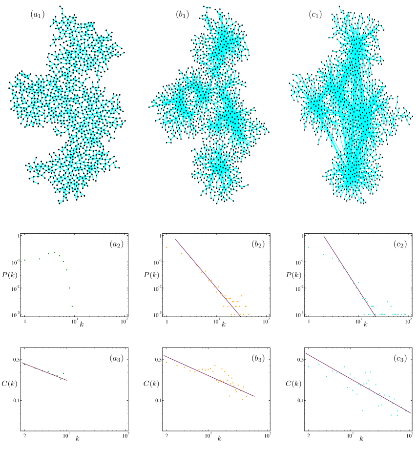
Figure 1: ($a_{1}$), ($b_{1}$), and ($c_{1}$): graphical representations of the models ($a$), ($b$), and ($c$), respectively. The three networks have $1000$ vertices; their size is $L=1881$ ($a_{1}$), $L=1982$ ($a_{2}$), and $L=1982$ ($a_{3}$). Note that all edges of network ($a_{1}$) are short-range connections, while in network ($c_{1}$) edges connecting distant vertices do exist. ($a_{2}$), ($b_{2}$), and ($c_{2}$): Degree distribution of the networks represented in ($a_{1}$), ($a_{2}$), and ($a_{3}$), respectively. Models ($b$) and ($c$) are scale-free. The slope of the straight lines are -2.24 ($b_{2}$) and -2.95 ($c_{2}$). ($a_{3}$), ($b_{3}$), and ($c_{3}$): Local clustering coefficient $C(k)$ of the networks represented in ($a_{1}$), ($a_{2}$), and ($a_{3}$), respectively. The behaviour of $C(k)$ follows power laws for three models. The slope of the straight lines are -0.40 ($a_{3}$), -0.46 ($b_{3}$) and -0.58 ($b_{3}$). Notice the double logarithmic scales in all graphs.

These basic ideas can be implemented in very different ways giving rise to different growth models. Consider, for instance, the preferential attachment prescription. One has to decide whether the attachment probability depends linearly on the degree, as in the Barabási-Albert construction Barabasi1 , or whether it must follow another law. One also has to decide about the interaction’s dependence on distance and on vertex attractiveness. Moreover, the probability of the appearance of a new vertex at position $\mathbf{r}$ can be a complex function involving the positions of all already existing vertices in the network, or depending only on the position of the vertices closer to the point.

The appropriate implementation of a determined pattern depends obviously on the particular geographical system that we attempt to model. Numerical simulations show that different (but similarly oriented) prescriptions produce models showing qualitatively the same behavior. This fact supports the general value of the principles proposed. Since we are not yet intending to studying any particular real-world network, but are interested only in capturing some general features of spatial systems, we will adopt here the simplest realization of the guiding prescriptions.

We start from a preselected area in a two-dimensional Euclidean plane. In this area, we place at random $m_{o}$ vertices, so that the distance between any two of these initial vertices is larger than a given $r_{min}$, the minimum distance that will separate vertices in the network. Since the $m_{o}$ vertices are placed at random, the order of magnitud of separation between them depends on the size of the preselected area. Now we let our network grow around these initial vertices. At each time step a new vertex with $m_{1}$ proper links is added to the network and connected to $m_{1}$ vertices already present. Additionally, once the new vertex is attached, $m_{2}$ new edges are distributed among all the vertices of the network. In both cases, vertices and edges are added to the network only if the geographical constraints allow for the addition.

Our geographic constraints are defined by the two characteristic distances $r_{min}$ and $r_{max}$, which define a ring area around a point. At each step we choose at random a vertex of the preexisting network. From this point, using polar coordinates, we put a new vertex at a position given by a radius $r$ and an angle $\phi$ picked up at random from homogeneous distributions $r_{min}\leq r\leq r_{max}$ and $\phi\in\left]0,2\Pi\right]$. If this new vertex happens to be at a distance smaller than $r_{min}$ from some preexisting one, the selection is rejected and a different old vertex is chosen. Note that this prescription does not give an homogeneous distribution in space when $r_{max}\to\infty$ and $r_{min}\to 0$, but essencially means that smaller distancies to the choosen vertex are preferred.

In order to connect the new vertex to the system, we consider the nodes of the network within the circle of radius $r_{max}$ from the newly introduced one $n$. This circular area around the new node is considered to be its physical neighborhood. If the number of vertices in the neighborhood is smaller than $m_{1}$, the newly introduced vertex is connected to all of them; if their numer exceeds $m_{1}$ than it is connected to exactly the $m_{1}$ ones with higher degree. Note that the fact that the range of the neighbourhood is precisely $r_{max}$ ensures that a new node is connected to at least one old one.

The second process, consisting of the addition of new edges between vertices, works in a similar way. We randomly choose a vertex $v$ of the network, and then, from the vertices that belong to its physical neighbourhood but are not yet connected to it, we choose the $m_{2}$ vertices having larger degree and connect $v$ to them. Here, however, the interaction range $r_{v}$ of the neighbourhood of $v$ is governed by the function

$$r_{v}=r_{max}+\beta{k_{v}}^{\gamma}\ ,$$ (1)

where $k_{v}$ is the degree of vertex $v$, and $\beta$ and $\gamma$ are non-negative tuning parameters whose function is basically to define the area which a vertex “sees” depending on its importance (degree) within the network. In case that the number of vertices that belong to the neighbourhood of $v$, and that are not yet connected to it, is $q<m_{2}$, then only $q$ edges are added to the network. Note that the effects of geography disappear when $r_{max}\to\infty$.

Let us comment on some aspects of the model. First, vertices are not distributed at random over the area of study, but their distribution depends on the “history” of the network. New vertices appear in the vicinity of the vertices already present in the network. Second, the interaction range of a vertex is a function of its attractiveness, or importance in the network. If a vertex increases its importance in the network, then its interaction range grows. (Here, we do not take into account the fact that old vertices can remain obsolete with time.) Third, we impose the following preferential attachment condition: connect to the more attractive vertex of the network that you can “see”.

Extensive numerical simulations confirm that this simple model is able to reproduce many of the properties of spatial networks. In the present study we restrict ourselves to two sets of values for the parameters of the model. The first one, which includes three different spatial cases, illustrates the impact of the cost-distance dichotomy on network structure. We consider the following values: $m_{1}=1$, $m_{2}=1$, $r_{min}=500$ m.u., and $r_{max}=1000$ m.u. (where m.u. stands for an arbitrary “metric unit”). The fact that we impose $r_{max}=2\cdot r_{min}$, i. e., that $r_{max}$ is only twice $r_{min}$, indicates that in this case we deal with networks for which the cost of new vertices establishing long-range connections is very high. Additionally, we choose $m_{0}=7$, and a radius of $14000$ m.u. for our initially preselected disc-area, within which the $m_{0}=7$ initial vertices may be placed at random. The three cases we distinguish are: Case ($a$), $\beta=1$ and $\gamma=1.4$, corresponding to a spatial network in which the geographical constraints are extremely important (in this case long-range connections are practically inexistent); Case ($b$), $\beta=1.5$ and $\gamma=2.3$, an intermediate case; Case ($c$), $\beta=2$ and $\gamma=4$, for which vertices of high degree are allowed to establish long-range connections. The selected values of parameters are certainly arbitrary and are adopted in order to illustrate the effects of the distance-cost-dependence. In effect, for $\beta=0$, the resulting network is practically a tree, since no edges can be placed between old vertices, while for very large $\beta$ and $\gamma$ a “winner-takes-all” phenomenon emerges, in which almost all vertices are connected to one super-hub with an enormous degree.

Figure 1 compares the results of simulations corresponding to these three cases. To be able to draw the resulting networks, we consider small graphs with only $1000$ vertices (numerical simulations indicate that the structure does not significantly change as the order of the networks grows). Panels $a_{1}$, $b_{1}$, and $c_{1}$ show the effects of the selective growth of the interaction range with the degree of vertices: For systems where long-range connections are highly expensive (model $a$), even the most important vertices of the network are connected only to a few close neighbours. As the cost of establishing long-range interactions decreases, connections between distant vertices in the network begin to appear, in particular, between high degree vertices (models $b$ and $c$).

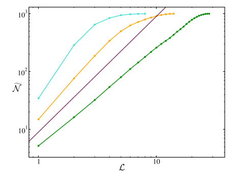
Figure 2: $\overline{\mathcal{N}}(\mathcal{L})$ as a function of the $\mathcal{L}$. From bottom to top, models $a$, $b$, and $c$. The black straight line correspond to a network of dimension $2$. The results are used to estimate the dimension of the three spatial networks considered (see text for more details). Notice the double logarithmic scales of the picture.

The degree distribution evidently changes as the geographical constraints are gradually loosened. Thus, model $a$ shows a degree distribution which decays approximately exponentially (panel $a_{2}$); no vertices of high degree can be found. The degree distributions of models $b$ and $c$, however, exhibit well-defined power law tails (in spite of the small order of the networks considered): $P(k)\sim k^{-2.25}$ (panel $b_{2}$) and $P(k)\sim k^{-2.95}$ (panel $c_{2}$). The corresponding local clustering coefficients also show a behaviour very close to that found in real networks (see panels $a_{3}$, $b_{3}$, and $c_{3}$). All three models exhibit power law behaviours for $C(k)$: $C(k)\sim k^{-0.40}$ (panel $a_{3}$), $C(k)\sim k^{-0.46}$ (panel $b_{3}$), and $C(k)\sim k^{-0.58}$ (panel $c_{3}$). In addition, the mean clustering coefficient $C$ of these spatial models is always quite large, about $C\simeq 0.33$ for all three of them. The number of triangles (cycles of length three) in the network is, however, $668$ (model $a$), $1593$ (model $b$), and $1341$ (model $c$). On the other hand, the average path length decreases as the amount of long-range connections grows from $l=20.18$ (model $a$)to $l=8.83$ (model $b$) and $l=5.01$ (model $c$). This result is quite natural, and shows the transition from a quasi-planar graph with a structure quite similar to a lattice (model $a$) to a typical complex network structure found in most geographical networks (models $b$ and $c$).

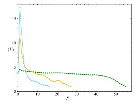
Figure 3: Layer average degree, $\langle k\rangle_{\mathcal{L}}$, as a function of shell number $\mathcal{L}$. The curve with the highest peak corresponds to model $c$, the intermediate one and the flat one to models $b$, and $a$, respectively.

Making use of the effective dimension $d$, Gastner and Newman showed that, networks where geographical effects are extreme are essentially planar graphs (i.e., they can be drawn on a map without any edges crossing). The effective dimension can be defined as $d=\lim_{\mathcal{L}\to\infty}\log{\overline{\mathcal{N}}(\mathcal{L})}/\log{\mathcal{L}}$, where $\overline{\mathcal{N}}(\mathcal{L})$ is the average number of vertices which can be found within a distance of $\mathcal{L}$ steps or less from a vertex. In finite networks no limit $\mathcal{L}\to\infty$ can be taken, but good results for $d$ can be achieved by plotting $\log{\overline{\mathcal{N}}(\mathcal{L})}$ against $\log{\mathcal{L}}$ for the central vertices of the network and measuring the slope of the resulting line (of course, far away of the saturation region corresponding to exhausting of the network). Central vertices are those vertices of the network that have minimum eccentricity, being defined as the maximum distance from the vertex to any other vertex in the network. (Note that central vertices are sometimes defined as the vertices having larger “betweenness centrality”, as in Guimera1 . We use, however, the classical definition from the graph theory.)

Figure 2 shows on double logarithmic scales how $\overline{\mathcal{N}}(\mathcal{L})$ behaves as a function of $\mathcal{L}$. From bottom to top the curves correspond to model ($a$), the critical behaviour $\overline{\mathcal{N}}(\mathcal{L})\sim{\mathcal{L}}^{2}$, model ($b$), and model ($c$). We see that the effective dimension of model $a$ is certainly smaller than two, which is not a surprize provided that model $a$ creates practically a planar graph. The dimensions of models $b$ and $c$ -which are obviously not planar graphs- are larger than two. The difference between the three models at $\overline{\mathcal{N}}(\mathcal{L}=1)$ is due to the fact that central vertices are usually the more connected ones of the network.

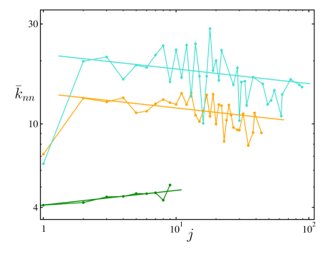
Figure 4: Analysis of the degree-degree correlations of the three models considered. Nearest neighbours’ average function $\overline{k}_{nn}(j)$ against $j$. From bottom to top, models $a$, $b$, and $c$. Note that models $b$ and $c$ exhibit dissortative mixing, while model $a$ is slightly assortative.

Tomographic studies reveal interesting details too. Tomography deals with the study of the structure of layers which surround a given vertex (the root) in the network Kalisky1 ; Xulvi-Brunet2 ; Volz1 . The principal motivation for examining the tomography of a network results from its importance for understanding the spreading phenomena taking place in networks. We concentrate here on the layer average degree $\langle k\rangle_{\mathcal{L}}=\sum_{k}kP_{\mathcal{L}}(k)$, where $P_{\mathcal{L}}$, the degree distribution in shell $\mathcal{L}$, is defined as $P_{\mathcal{L}}(k)=(\sum_{r}N_{\mathcal{L},r}(k))/(\sum_{k,r}N_{\mathcal{L},r}(k))$, with $N_{\mathcal{L},r}(k)$ being the number of vertices of degree $k$ in layer $\mathcal{L}$ for root $r$. The study of $\langle k\rangle_{\mathcal{L}}$ for the three networks considered shows a peak whose height decreases as the cost of establishing long-range connections grows (fig. 3). The results indicate that the mean degree $\langle k\rangle_{\mathcal{L}=1}$ increases rapidly as the number of long-range connections and hubs in the network grows. On the other hand, the average shell degree decreases rapidly for more distant layers, $\mathcal{L}>1$. This interesting result shows that vertices with large degrees are rapidly exhausted in this type of networks, which has especial importance when dealing with spreading phenomena, like spreading of information or infections. Note that this result has important effects on epidemiological properties: vertices of large degree are rapidly affected by the spreading of an infection. On the other hand, in a network like that of model ($a$) the propagation of any spreading agent will be similar to the propagation on a lattice: the spreading agent will primarily reach the nearest physical neighbours.

In figure 4 we show the correlation properties of these three models. Degree-degree correlations are determined by the probability function $\mathcal{E}_{ij}$, which gives the probability that a randomly selected edge connects one vertex of degree $i$ to another of degree $j$. Thus, a network is said to be degree-degree uncorrelated if $\mathcal{E}_{ij}=(2-\delta_{ij})iP(i)jP(j)/\langle i\rangle^{2}$, which only means that the probability that an edge connects to a vertex of a certain degree $k$ is independent from whatever vertex is attached to the other end if the edge. Otherwise, the network is said to be degree-degree correlated. Most real networks are correlated, and usually exhibit either “assortative” or “dissortative” mixing Newman1 . Assortativity means that high-degree vertices attach preferably to other highly connected vertices, i. e., with a larger probability than in uncorrelated networks; on the other hand, dissortativity stands for when high-degree vertices tend to connect to low-degree vertices, and vice versa. Thus, a very useful quantity for measuring the correlation’s degree of a network is the nearest neighbours’ average function $\overline{k}_{nn}(j)$, which expressed in terms of $\mathcal{E}_{ij}$, can be written as $\overline{k}_{nn}(j)=(\sum_{i}i(1+\delta_{ij})\mathcal{E}_{ij})/(\sum_{i}(1+\delta_{ij})\mathcal{E}_{ij})$. It takes the constant value $\overline{k}_{nn}(j)=\langle j^{2}\rangle/\langle j\rangle$ if no type of degree-degree correlation exist, while it is a decreasing (increasing) function if dissortative (assortative) mixing is present. In the picture we plot $\overline{k}_{nn}(j)$ as a function of $j$. The lowest curve, corresponding to model ($a$), shows then that the network is slightly assortative. This feature of model ($a$) is due to the fact that the areas containing a large density of vertices usually contain a large density of edges (see Figure 1, $a_{1}$), corresponding probably to important areas of the space; and vice versa, the areas containing a small density of vertices also contain a small density of edges. On the other hand, models ($b$) and ($c$), in which the geographical constraints are not so strong, present dissortative mixing. Interestingly, for both models $\overline{k}_{nn}(j)$ falls with $j$ following power laws of the form $\overline{k}_{nn}(j)\sim j^{-\iota}$, just like happens in real networks.

Model ($a$) reproduces quite well the properties of those systems where vertices and edges are embedded in the two-dimensional physical space, like, for example, electric power grids or road networks. However, none of the three models considered above is suitable for characterising world-scale systems such as the Internet or the network of airline routes. The reason is that, in such large-scale systems, vertices are usually not uniformly distributed in the region under study (as occurs in our preceding models, see pictures 1 $a_{1}$, $b_{1}$, and $c_{1}$), but they concentrate in a number of technological areas distributed over the world. Thus, a more realistic model for describing such systems must take into account that in large-scale geographical networks there usually exist many “desert” regions lying between the areas where vertices can be found in abundace. Such a pattern is easy to construct by varying the ratio between $r_{max}$ and $r_{min}$ in our model. This aspect is actually considered by our second selection of parameters. As we will see next, inhomogeneous distribution of vertices in space influences quantitatively the statistical properties of networks.

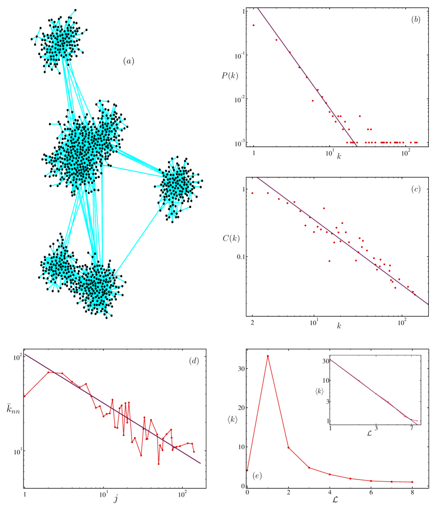
Figure 5: ($a$): Graphical representation of a small network ($N=1000$ and $L=1985$) corresponding to model ($d$). Note that vertices concentrate in certain areas of the space, and that the long-range connections of the network link end-vertices of large degree. ($b$): Degree distribution of model ($d$). ($c$): Degree-dependent clustering coefficient $C(k)$ of the model. ($d$): nearest neighbours’ average function $\overline{k}_{nn}$ as function of the degree $j$. Note that $P(k)$, $C(k)$, and $\overline{k}_{nn}$ fall off as power law functions. ($e$): Average degree, $\langle k\rangle_{\mathcal{L}}$, as a function of shell number $\mathcal{L}$. From $\langle k\rangle_{\mathcal{L}=1}$ the average degree decays interestingly following a power law (inset of the picture).

blanc blanc blanc blanc blanc blanc blanc blanc blanc

Let us thus consider a larger ratio for $r_{max}/r_{min}$, for example, $r_{max}=5\cdot r_{min}$. (Note that the change in the ratio $r_{max}/r_{min}$ modifies not only the distribution of vertices in space, but also makes cheaper the cost of establishing connections for new vertices, since the neighbourhood of a new vertex will, in comparison, contain more vertices.) The values of the parameters for this model (model $d$) are now the following: $m_{0}=7$, $m_{1}=1$, $m_{2}=1$, $r_{min}=200$ m. u., $r_{max}=1000$ m. u., $\beta=2$ and $\gamma=3$. As before, the initial area, where the $m_{0}=7$ vertices are randomly placed, has a radius of $14000$ m. u. and the order of the network is $N=1000$. Figure 5 ($a$) shows this network in the two-dimensional Euclidean space: The model simulates perfectly the tendency of vertices to concentrate in different areas having a high density of vertices (as if these areas were urban centres, i.e., cities, or city agglomerations), which are linked through long-range connections which join vertices of large degree, usually belonging to different geographical communities.

The properties of this last construction are especially interesting, since they reproduce many structural properties found in the Internet. Thus, the degree distribution of the model follows a power law $P(k)\sim k^{-2.42}$ (panel $b$ of figure 5). The mean clustering coefficient is large. For our small network $C\simeq 0.7$. The degree-dependent clustering coefficient $C(k)$ decays as a power law function $C(k)\sim k^{-0.97}$ (panel $c$ of the Figure). The decay of $C(k)$ gets however slower for networks of larger size $N$. The average path length is very small, $l=3.74$ for the parameters as in Figure 5, and numerical simulations with larger networks indicate a small-world behaviour. In addition, the network shows dissortative mixing: the nearest neighbours’ average function $\overline{k}_{nn}$ decreases as $\overline{k}_{nn}(j)\sim j^{-0.52}$ (see Fig. 5 $d$). The coincidence of these properties with the ones of the Internet is astonishing: Let us now remind that i) the degree distribution of the Internet follows a power law with exponent $\gamma\simeq-2.5$, ii) the local clustering function $C(k)$ behaves as $C(k)\sim k^{-0.75}$, and iii) $\overline{k}_{nn}$ decreases with $j$ following the function $\overline{k}_{nn}(j)\sim j^{-0.5}$ Vazquez1 . Finally, in Figure 5 we plot ($e$) the average degree $\langle k\rangle_{\mathcal{L}}$ as a function of shell number $\mathcal{L}$, corresponding to the study of tomography. We see again that hubs are found only a few steps away from any vertex, and interestingly, that $\langle k\rangle_{\mathcal{L}}$ drops as a perfect power law from $\mathcal{L}=1$ on (see inset of the Figure; note the double logarithmic scales).

To conclude, we introduce several network-generating mechanisms taking into account the constraints that geography impose on the evolution of large-scale network systems in physical space. We suggest that two properties are determinant for the structure of such geographical networks: the fact that the spatial interaction range of vertices depends on the vertex attractiveness and the fact that that vertices are not randomly distributed in space. Simple implementations of these mechanisms show that the essential difference between “strong geographical” networks, such as electric power grids, and “weak geographical” networks, such as the Internet or the airline network, could be the cost (economical or technological) of establishing long-range connections. On the other hand, inhomogeneous distribution of vertices in large-scale networks seems certainly to be a relevant generating element of their hierarchical character. In any case, the agreement of our results with the properties found in real networks suggest that the mechanisms proposed may play a key role in the evolution and structure of networks.

References

- (1) M. E. J. Newman, SIAM Rev. 45, 167 (2003).
- (2) S.-H. Yook, H. Jeong, and A.-L. Barabási, PNAS 99, 13382 (2002).
- (3) A. Vázquez, R. Pastor-Satorras, and A. Vespignani, Phys. Rev. E 65, 066130 (2002).
- (4) L. A. N. Amaral, A. Scala, M. Barthélemy, and H. E. Stanley, Proc. Natl. Acad. Sci. USA 97, 11149 (2000).
- (5) R. Guimerà, S. Mossa, A. Turtschi, and L. A. N. Amaral, Proc. Natl. Acad. Sci. USA 102, 7794 (2005).
- (6) M. T. Gastner and M. E. J. Newman, Eur. Phys. J. B 49, 247 (2006).
- (7) V. Latora and M. Marchiori, Physica A 314, 109 (2002).
- (8) P. Sen, S. Dasgupta, A. Chatterjee, P. A. Sreeram, G. Mukherjee, and S. S. Manna, Phys. Rev. E 67, 036106 (2003).
- (9) D. J. Watts and S. H. Strogatz, Nature 393, 440 (1998).
- (10) R. Albert and A.-L. Barabási, Rev. Mod. Phys. 74, 47 (2002).
- (11) S.N. Dorogovtsev and J.F.F. Mendes, Adv. Phys. 51, 1079 (2002).
- (12) S. Boccaletti, V. Latora, Y. Moreno, M. Chavez, and D.-U. Hwang, Phys. Rep. 424, 175 (2006).
- (13) R. Xulvi-Brunet and I. M. Sokolov, Phys. Rev. E 66, 026118 (2002).
- (14) S. S. Manna and P. Sen, Phys. Rev. E 66, 066114 (2002).
- (15) J. Jost and M. P. Joy, Phys. Rev. E 66, 036126 (2002).
- (16) A. F. Rozenfeld, R. Cohen, D. ben-Avraham, and S. Havlin, Phys. Rev. Lett. 89, 218701 (2002).
- (17) C. P. Warren, L. M. Sander, and I. M. Sokolov, Phys. Rev. E 66, 056105 (2002).
- (18) J. Dall and M. Christensen, Phys. Rev. E 66, 016121 (2002).
- (19) M. Barthélemy, Europhys. Lett. 63, 915 (2003).
- (20) C. Andersson, A. Hellervik, K. Lindgren, A. Hagson, and J. Tornberg, Phys. Rev. E 68, 036124 (2003).
- (21) P. Sen and S. S. Manna, Phys. Rev. E 68, 026104 (2003).
- (22) S. S. Manna and A. Kabakçioğlu, J. Phys. A: Math. Gen. 36, 279 (2003).
- (23) C. Herrmann, M. Barthélemy, and P. Provero, Phys. Rev. E 68, 026128 (2003).
- (24) D. ben-Avraham, A. F. Rozenfeld, R. Cohen, and S. Havlin, Physica A 330, 107 (2003).
- (25) M. Kaiser and C.C. Hilgetag, Phys. Rev. E 69, 036103 (2004).
- (26) K. Yang, L. Huang, and L. Yang, Phys. Rev. E 70, 015102 (2004).
- (27) J. P. K. Doye and C. P. Massen, Phys. Rev. E 71, 016128 (2005).
- (28) L. Huang, L. Yang, and K. Yang, Europhys. Lett. 72, 144 (2005).
- (29) J. J. S. Andrade, H. Herrmann, R. F. S.Andrade, and L. R. da Silva, Phys. Rev. Lett. 94, 018702 (2005).
- (30) A. Barrat, A., M. Barthélemy, and A. Vespignani, J. Stat. Mech. P05003 (2005).
- (31) N. Masuda, H. Miwa, and N. Konno, Phys. Rev. E 71, 036108 (2005).
- (32) Y. Hayashi and J. Matsukubo, Phys. Rev. E 73, 066113 (2006).
- (33) Y. Hayashi, IPSJ Digital Courier, Vol. 2, 155 (2006).
- (34) P. Crucitti, V. Latora, and S. Porta, Phys. Rev. E 73, 036125 (2006).
- (35) Y. Roudi and A. Treves, Phys. Rev. E 73,061904 (2006).
- (36) A. Cardillo, S Scellato, V. Latora, and S. Porta, Phys. Rev E 73, 066107 (2006).
- (37) M. T. Gastner and M. E. J. Newman, Phys. Rev. E 74, 016117 (2006).
- (38) A.-L. Barabási, and R. Albert, Science 286, 509 (1999).
- (39) T. Kalisky, R. Cohen, D. ben-Avraham, and S. Havlin. Lect. Notes Phys. 650, 3 (2004).
- (40) R. Xulvi-Brunet, W. Pietsch, and I. M. Sokolov, Phys. Rev. E 68, 036119 (2003).
- (41) E. Volz, arXiv:physics/0509129 (2005).
- (42) M. E. J. Newman, Phys. Rev. E 67, 026126 (2003).