General radar transmission codes that minimize measurement error of a static target

Abstract

The variances of matched and sidelobe free mismatched filter estimators are given for arbitrary coherent targets in the case of aperiodic transmission. It is shown that mismatched filtering is often better than matched filtering in terms of estimation accuracy. A search strategy for finding general transmission codes that minimize estimation error and satisfy constraints on code power and amplitude range is then introduced. Results show that nearly perfect codes, with performance close to a single pulse with the same total power can be found. Also, finding these codes is not computationally expensive and such codes can be found for all practical code lengths. The estimation accuracy of the newly found codes are compared to binary phase codes of similar length and found to be better in terms of estimator variance. Similar transmission codes might be worth investigating also for sonar and telecommunications applications.

I Introduction

Phase modulation of a radar transmission is a well known method for increasing radar transmission power, while still maintaining a good range resolution. Such transmission codes can consist of two or more individual phases. The performance of binary, quadri and polyphase codes has been thoroughly inspected in terms of heuristic criteria, such as the integrated sidelobe level (ISL), or peak to sidelobe level (PSL) [1, 2, 3, 5, 4, 6, 7]. In previous work, binary phase codes have also been evaluated in terms of estimation accuracy of a static target, when using an optimal sidelobe free mismatched filter for periodic [8, 9, 12] and aperiodic signals [10].

We first examine the behaviour of matched and optimal sidelobe free mismatched filter estimators for a point like and a uniform target. In the case of a point-like target, we get the well known result that the matched filter is optimal, and the sidelobe free mismatched filter has a larger estimator variance, which depends mainly on the sidelobe power, and is thus not necessarily very high. In the case of a uniform target, we see that the matched filter produces biased results and in addition to the bias, it also has a worse estimator variance in many cases. (Here we consider the mean value of the error term as bias and call the second moments of the error term around the mean the estimator variance).

II General transmission code

A code with length $L$ can be described as an infinite length sequence with a finite number of nonzero pulses with phases and amplitudes defined by parameters $\phi_{k}$ and $a_{k}$. These parameters obtain values $\phi_{k}\in[0,2\pi]$ and $a_{k}\in[a_{\mathrm{min}},a_{\mathrm{max}}]$, where $k\in[1,\ldots,L]:k\in\mathbb{N}$. The reason why one might want to restrict the amplitudes to some range stems from practical constraints in transmission equipment. In most traditional work, the amplitudes have been set to $1$ and often the number of phases has also been restricted, eg., in the case of binary phase codes to $\phi_{k}\in\{0,\pi\}$.

Defining $\delta(t)$ with $t\in\mathbb{Z}$ as

$$\delta(t)=\left\{\begin{array}[]{lcr}1&\mbox{when}&t=0\\ 0&\mbox{otherwise}&\end{array}\right.$$ (1)

we can describe an arbitrary baseband radar code $\epsilon(t)$ as

$$\epsilon(t)=\sum_{k=1}^{L}a_{k}e^{i\phi_{k}}\delta(t-k+1).$$ (2)

In addition to this, we restrict the total transmission code power to be constant for all codes of similar length. Without any loss of generality, we set code power equal to code length

$$L=\sum_{t=1}^{L}|\epsilon(t)|^{2}.$$ (3)

This will make it possible to compare estimator variances of codes with different lengths and therefore different total transmission powers. Also, it is possible to compare codes of the same length and different transmission power simply by treating $L$ as transmission power.

III Measurement equation

Equation 4 describes the basic principle of estimating a coherent radar target using a linear filter. When the target is assumed to be infinite length and using roundtrip time as range, the scattering from a target is simplified to convolution of the transmission with the target. In this convolution equation, $m(t)$ denotes the measured signal, $\sigma(t)$ denotes the unknown target, $\epsilon(t)$ denotes the transmitted waveform and $\xi(t)$ represents thermal noise, which is assumed to be Gaussian white noise with power $\mathrm{SNR}^{-1}$. Finally, $h(t)$ represents the decoding filter used to decode the signal, it can be eg., a matched or mismatched filter.

$$m(t)=\left[\sigma(t)\ast\epsilon(t)+\xi(t)\right]\ast h(t)$$ (4)

Assuming that the Fourier transformation of the transmitted waveform contains no zeros, a solution to the previous equation can be found easily in frequency domain [10]. Using notation $\mathcal{F}_{D}\left\{\epsilon(t)\right\}=\hat{\epsilon}(\omega)$ for a zero padded discrete Fourier transform with transform length $M\gg L$, the optimal sidelobe free mismatched filter can be defined as $\mathcal{F}_{D}^{-1}\left\{L/\hat{\epsilon}(\omega)\right\}=\lambda(t)$. Such a filter will be infinite length, but it is a mathematical fact that the coefficients will exponentially approach zero [11], so one can use a truncated $\lambda(t)$ with errors of machine precision magnitude. Also, it is known that filtering with $\lambda(t)$ is the minimum mean square estimator for target amplitude.

In the case of the mismatched filter, we set $h(t)=\lambda(t)$ in the measurement equation, which can be simplified into the following form

$$m_{\lambda}(t)=L\sigma(t)+\underbrace{(\xi\ast\lambda)(t)}_{\mathrm{measurement\ error}}.$$ (5)

In the case of a matched filter $h_{m}(t)=\overline{\epsilon(-t)}$, one can also extract the target from the measurement equation. From equation $(\epsilon*h_{m})(t)-r(t)=L\delta(t)$, we see that the matched filter can be expressed using the mismatched filter $\lambda(t)$ and code autocorrelation function sidelobes $r(t)$ as

$$h_{m}(t)=\lambda(t)+\frac{1}{L}(\lambda*r)(t),$$ (6)

and thus we can write the matched filter measurement equation $m_{m}(t)$ as

$$m_{m}(t)=L\sigma(t)+(r*\sigma)(t)+\underbrace{(\xi\ast h_{m})(t)}_{\mathrm{measurement\ error}}.$$ (7)

Equation 6 shows that the matched filter for a code with integrated sidelobe power approaching zero $\sum_{t=-\infty}^{\infty}|r(t)|^{2}\rightarrow 0$ approaches the sidelobe free mismatched filter $h_{m}(t)\rightarrow\lambda(t)$. In this case measurement equations 5 and 7 are the same, which is a natural result. Figure 1 shows a mismatched and a matched filter for a relatively good code.

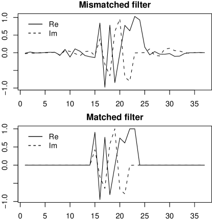
Figure 1: The mismatched and matched filters of a polyphase code $\phi_{k}\in[0,2\pi]$ with length $L=9$ and $R=0.974$.

IV Estimators

When estimating the power of a target, it is customary to use several repetitions of a measurement. In this case, the target and the thermal noise are denoted as random variables, which are indexed with $q\in\mathbb{N}$, ie., each repetition is a different random variable. The measurement equation for repeated measurements is then written as

$$m^{q}(t)=\left[(\epsilon*\sigma^{q})(t)+\xi^{q}(t)\right]*h(t).$$ (8)

Even though the scattering amplitude and thermal noise amplitude change between measurements, we assume that the statistical properties of the thermal noise and the target are unchanged between measurements, and this is what is estimated. The target is measured as target power using sample variance, from which we subtract known bias caused by the thermal noise entering the filter. The matched filter target power estimator is thus

$${\hat{x}_{\mathrm{mat}}}(t)=-\frac{{B_{\mathrm{mat}}}}{L^{2}}+\frac{1}{N\,L^{2}}\sum_{q=1}^{N}|m_{m}^{q}(t)|^{2}$$ (9)

and the mismatched filter

$${\hat{x}_{\mathrm{mis}}}(t)=-\frac{{B_{\mathrm{mis}}}}{L^{2}}+\frac{1}{N\,L^{2}}\sum_{q=1}^{N}|m_{\lambda}^{q}(t)|^{2}.$$ (10)

In these equations the thermal noise entering the filter is denoted with ${B_{\mathrm{mat}}}=\mathrm{SNR}^{-1}\sum_{\tau=-\infty}^{\infty}|h_{m}(\tau)|^{2}$ and ${B_{\mathrm{mis}}}=\mathrm{SNR}^{-1}\sum_{\tau=-\infty}^{\infty}|\lambda(\tau)|^{2}$.

V Point-like target

In baseband, the scattering from a point target is defined as a zero mean complex Gaussian random process with the second moment defined with the following expectation

$$\mathrm{E}\,\sigma^{q}(t)\overline{\sigma^{p}(t^{\prime})}=x\delta(t-t_{c})\delta(t^{\prime}-t_{c})\delta(q-p).$$ (11)

In other words, the scattering is zero for all other ranges than $t_{c}$, where the scattering power is $x$. Different repetitions are not correlated.

In this case, it can be shown that the matched filter and mismatched filter estimators are both unbiased, ie., $\mathrm{E}\,{\hat{x}_{\mathrm{mis}}}(t)=\mathrm{E}\,{\hat{x}_{\mathrm{mat}}}(t)=x$. The estimator variances are:

$$\mathrm{Var}\,\hat{x}_{\mathrm{mat}}=\frac{1}{N}\left(x^{2}+\frac{2{B_{\mathrm{mat}}}x}{L^{2}}+\frac{{B_{\mathrm{mat}}}^{2}}{L^{4}}\right)$$ (12)

and

$$\mathrm{Var}\,\hat{x}_{\mathrm{mis}}=\frac{1}{N}\left(x^{2}+\frac{2{B_{\mathrm{mis}}}x}{L^{2}}+\frac{{B_{\mathrm{mis}}}^{2}}{L^{4}}\right).$$ (13)

The target itself is a source of estimation errors, as it is a Gaussian random variable (self-noise). The only code dependent terms are the thermal noise terms ${B_{\mathrm{mat}}}$ and ${B_{\mathrm{mis}}}$. Thus, the only way to reduce estimator variance is to reduce thermal noise. In the case of a matched filter, the noise entering the filter is independent of the code and proportional decoding filter power $L$. For a mismatched filter, the thermal noise term is always larger than the matched filter equalent, and it is highly code dependent. In order to compare estimator performance, we can use the following ratio:

$$R=\frac{{B_{\mathrm{mat}}}}{{B_{\mathrm{mis}}}}=\frac{L}{\sum_{\tau=-\infty}^{\infty}|\lambda(\tau)|^{2}},$$ (14)

which will approach $1$ when the performance of the optimal mismatched filter approaches that of the matched filter.

VI Distributed target

When the target is not point-like, the situation is different. A zero mean time-stationary Gaussian scattering medium with power depending on range can be defined as

$$\mathrm{E}\,\sigma^{q}(t)\overline{\sigma^{p}(t^{\prime})}=x(t)\,\delta(t-t^{\prime})\,\delta(q-p).$$ (15)

Figure 2. shows an example of $x(t)$ and the instantanious scattering $\sigma(t)$.

Figure 2: The expectation of power and an example of an instance of the target.

In the case of a distributed target, it can be shown that the expectation of the matched filter estimator is biased, with the sidelobes convolved with the target. By defining the sidelobe term as

$$S(t)=\sum_{\tau=-\infty}^{\infty}|r(\tau)|^{2}x(\tau-t),$$ (16)

we can describe the matched filter estimator mean as

$$\mathrm{E}\,\hat{x}_{\mathrm{mat}}(t)=x(t)+\frac{S(t)}{L^{2}}.$$ (17)

On the other hand, the sidelobe free mismatched filter estimator is unbiased. It has mean

$$\mathrm{E}\,\hat{x}_{\mathrm{mis}}(t)=x(t).$$ (18)

The variance of the estimators can also be found. The matched filter has a variance

$$\mathrm{Var}\,\hat{x}_{\mathrm{mat}}(t)= \frac{1}{N}\Big{[}x(t)^{2}+\frac{2{B_{\mathrm{mat}}}\,x(t)}{L^{2}}+\frac{2S(t)x(t)}{L^{2}}+$$

$$\frac{{B_{\mathrm{mat}}}^{2}}{L^{4}}+\frac{S(t)^{2}}{L^{4}}+\frac{2{B_{\mathrm{mat}}}\,S(t)}{L^{4}}\Big{]}$$ (19)

and the mismatched filter has variance:

$$\mathrm{Var}\,\hat{x}_{\mathrm{mis}}(t)=\frac{1}{N}\left[x(t)^{2}+\frac{2{B_{\mathrm{mis}}}\,x(t)}{L^{2}}+\frac{{B_{\mathrm{mis}}}^{2}}{L^{4}}\right]$$ (20)

By inspecting these equations, one can see that the mismatched filter variance is the same as it was for a point-like target, but the matched filter has additional sidelobe terms. In many cases these terms will cause the variance of the matched filter estimator to be wider than the mismatched filter estimator variance.

Figure 3 shows a simulated target that is probed with a random phase code and then the target power is estimated with matched and mismatched filter estimators. A relatively poor random phase code with $R=0.23$ was used to emphasize the following relevant features:

1. With all but the smallest signal to noise ratios the matched filter estimator has larger variance. For example, if the target is assumed to be completely uniform $x(t)=1$, the matched filter estimator variance for the 13-bit Barker code is better only when $\mathrm{SNR}<0.05$. When the signal to noise ratio is higher than this, the mismatched filter has better estimation variance. When $\mathrm{SNR}=1$, the estimation variance of the mismatched filter is already $11$% better for the 13-bit Barker code.

2. The matched filter has bias which depends on the sidelobes. For example, when the target is again uniform $x(t)=1$, the bias of the best binary phase codes of lengths $3$ to $42$ is around $0.1$, in other words, the target power estimate is $10$% higher than it is in reality. In figure 3, the bias is about $80$%.

3. The mismatched filter produces larger thermal noise. This can be seen on the outermost extremes in Figure 3 where $x(t)=0$. This is code dependent, and depends on the value of $R$. When $R\rightarrow 1$, the thermal noise of a mismatched filter is equal to that of a matched filter.

Figure 4 shows the ratio of matched and mismatched filter variances for the best polyphase and binary phase codes of several different lengths as a function of signal to noise ratio. When the ratio is smaller than one, the matched filter performs better. It can be seen from the figure that when $\mathrm{SNR}$ is increased, the mismatched filter is better after some threshold $\mathrm{SNR}$, and the ratio of variances asymptotically approaches a certain code dependent ratio. Also, when code length is increased, the threshold $\mathrm{SNR}$ where the mismatched filter has better variance is lowered. This can be seen from the behaviour of the polyphase code of length 1024.

Figure 3: Simulated uniform target estimated with a matched and mismatched filter using a random phase code. In this case the signal to noise ratio is one, and the code is relatively poor $R=0.23$. The matched filter estimator has bias and larger variance due to self-noise caused by the target. The correct target is zero everywhere else and $x(t)=1$ when $t\in[90,290]\cup[300,590]$.

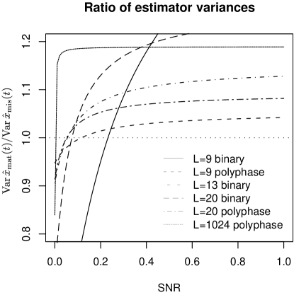
Figure 4: The ratio of matched and mismatched filter estimator variances for a uniform target $x(t)=1$. The best performing polyphase and binary phase codes for several code lengths is shown. When the ratio is $>1$, the mismatched filter estimator is better.

VII Code optimality

In our considerations, we only concentrate on minimizing the mismatched filter estimator variance, because the matched filter is biased by the code sidelobes and also often has larger estimator variance for a distributed target. In any case, it is possible to inspect matched filter estimator performance by using equation 19.

From the equations of mismatched filter estimator variance it is clear that the code affects estimation variance. The estimator variance is the same for both distributed and point targets, so it is sufficient to maximize the ratio $R$ described in equation 14. But what does maximizing $R$ mean? From eq. 6, which describes a matched filter in terms of a mismatched filter and matched filter ACF sidelobes $r(t)$, one can see that when sidelobe power $p=\sum_{t=-\infty}^{\infty}|r(t)|^{2}$ approaches zero the mismatched filter approaches the matched filter

$$\lim_{p\rightarrow 0}h_{m}(t)=\lambda(t).$$ (21)

In this case we have a code with $R=1$, ie., the matched and mismatched filters are the same and ACF is a single spike $\epsilon(t)*\overline{\epsilon(-t)}=L\delta(t)$. Therefore, even though we are restricting ourselves to the mismatched filter, the same codes will also be good when used as a matched filter. The closer $R$ is to $1$, the smaller the sidelobes and thus matched filter error.

Traditional code optimality criteria also reflect code goodness, but their relation to mismatched filter estimation accuracy is not that well defined. Still, it is evident from equation 6 that the sidelobes of the code autocorrelation function directly affect the performance of the mismatched filter by making the filter longer than the matched filter, allowing more thermal noise to enter the estimate. Thus, traditional code optimality criteria such as peak to maximum sidelobe level (PSL) or code power divided by integrated sidelobe power (MF) will also reflect code goodness. In the limiting case, when $PSL\rightarrow 0$ and $MF\rightarrow\infty$ it is clear that $R$ will also have limit $R\rightarrow 1$.

VIII Code search algorithm

  repeat

     for $b=1$ to $\mathrm{code\ length}$ do

        $\phi[b]\Leftarrow\mathrm{UniformRandom}(0,2\pi)$

        $a[b]\Leftarrow 1$

        $\epsilon[b]\Leftarrow a[b]*\exp(j\phi[b])$

     end for

     for $i=1$ to $\mathrm{number\ of\ iterations}$ do

        if $\mathrm{UniformRandom}(0,1)<0.5$ then

           $b\Leftarrow\mathrm{floor}(\mathrm{UniformRandom}(0,\mathrm{code\ length}))+1$

           $\Delta\phi\Leftarrow\mathrm{UniformRandom}(0,2\pi)$

           $\mathrm{old}\epsilon\Leftarrow\epsilon[b]$

           $\epsilon[b]\Leftarrow\exp(j\Delta\phi)$

           $NewR\Leftarrow\mathrm{CalculateR}(c)$

           if $NewR>R$ then

              $R\Leftarrow NewR$

              $\phi[b]\Leftarrow\Delta\phi$

           else

              $\epsilon[b]\Leftarrow\mathrm{old}\epsilon$

           end if

        else

           $b1\Leftarrow\mathrm{floor}(\mathrm{UniformRandom}(0,\mathrm{code\ length}))+1$

           $b2\Leftarrow\mathrm{floor}(\mathrm{UniformRandom}(0,\mathrm{code\ length}))+1$

           $\Delta{}a\Leftarrow\mathrm{NormalRandom}(0,1)$

           $\mathrm{olda}\Leftarrow a$

           $\mathrm{old}\epsilon\Leftarrow\epsilon$

           $q\Leftarrow 4a[b2]^{2}-8a[b1]\Delta{}a-4\Delta{}a^{2}$

           if $q>0\,\,\mathbf{and}\,\,b1<>b2$ then

              $\Delta{}a2\Leftarrow-a[b2]-0.5\sqrt{q}$

              $a[b1]\Leftarrow a[b1]-\Delta{}a$

              $a[b2]\Leftarrow a[b2]+\Delta{}a2$

              $c[b1]\Leftarrow a[b1]\exp(j\phi[b1])$

              $c[b2]\Leftarrow a[b2]\exp(j\phi[b2])$

              $NewR\Leftarrow\mathrm{CalculateR}(\epsilon)$

              if $NewR>R$ then

                 $R\Leftarrow NewR$

              else

                 $\epsilon\Leftarrow\mathrm{old}\epsilon$

                 $a\Leftarrow\mathrm{olda}$

              end if

           end if

        end if

     end for

  until R good enough

Algorithm 1 Random local improvement algorithm.

Lacking an analytic method of obtaining codes with $R$ close to one, while statisfying the constraint on code amplitude range $a_{k}\in[{a_{\mathrm{min}},a_{\mathrm{max}}}]$, we resort to numerical means. In order to get an overview of how the performance of codes is distributed among codes, we sampled several code lengths using $10^{6}$ randomly chosen polyphase codes (constant amplitude), and used a histogram to come up with an estimate distribution of R. This shown in figure 5. It is evident that as the code length grows, it becomes nearly impossible to find good codes by searching them in a purely random fashion. Therefore, in order to proceed numerically, some form of optimization algorithm was needed.

Figure 5: Distribution of R for random polyphase codes, ie., $a_{k}=1$ and $\phi_{k}\in[0,2\pi]$ for all $k$.

We used a heuristic optimization algorithm specifically created for this task, with the purpose of robustly converging to a maxima of $R$ as a function of a code, while satisfying constraints on code amplitude range. The code is described in algorithm 1. The idea is as follows:

1. We first generate a code with all bauds at random phases and unit amplitudes.

2. For a fixed amount of iterations, a new phase or amplitude is randomized for a randomly selected baud, and $R$ calculated for the resulting trial code. If the amplitude is changed, we also select another baud and change its amplitude in the opposite direction in order to maintain total code power at $L$. If the code is good enough, we select it as our new current working code.

3. After each “optimization run”, we will find a code at some local maximum. The optimization runs (Step 2.) are then repeated with new random initial code until a satisfactory result has been obtained.

The number of iterations of an optimization run is a tunable parameter of the algorithm, it varies from $10^{3}$ for small code lengths to $10^{6}$ for codes with length $L>10^{3}$.

One of the main reasons for robustness of this algorithm is that it does not follow the largest gradient, but instead follows a random positive gradient, making it more likely that more local maximas of $R$ are visited.

The algorithm has also been applied with some modifications for more resticted cases, such as binary and quadriphase codes that are too long to search exhaustively.

IX Search results

We applied the search algorithm for code lengths $3$ to $4096$ using three different amplitude ranges: $A_{1}:=[1,1]$, $A_{2}:=[0.95,1.05]$ and $A_{3}:=[0,2]$. The first of these is a polyphase code with constant amplitude, the other two allow a certain amount of amplitude deviation around 1. Results are shown in table I as the best value of $R$ found for given code length and amplitude range. For comparison, the values of best binary phase codes are also shown in column $B$. Some selected codes are given in table II..

TABLE I: Best transmission codes found.

Length	$A_{1}$	$A_{2}$	$A_{3}$	$B$
3	0.745	0.775	1.000	0.745
4	0.679	0.748	1.000	0.679
5	0.866	0.900	1.000	0.866
6	0.676	0.743	1.000	0.676
7	0.894	0.917	1.000	0.705
8	0.817	0.862	1.000	0.756
9	0.974	0.979	1.000	0.618
10	0.886	0.921	1.000	0.678
11	0.926	0.946	1.000	0.804
12	0.899	0.927	1.000	0.853
13	0.954	0.971	1.000	0.952
14	0.926	0.948	1.000	0.835
15	0.951	0.968	1.000	0.870
16	0.937	0.958	1.000	0.788
17	0.953	0.969	1.000	0.773
18	0.927	0.954	1.000	0.792
19	0.968	0.958	1.000	0.831
20	0.956	0.973	1.000	0.838
21	0.962	0.976	1.000	0.835
22	0.956	0.974	1.000	0.806
23	0.968	0.983	1.000	0.824
24	0.959	0.974	1.000	0.835
25	0.968	0.982	1.000	0.853
26	0.960	0.976	1.000	0.877
27	0.953	0.973	1.000	0.862
28	0.956	0.970	1.000	0.847
29	0.959	0.974	1.000	0.853
30	0.940	0.971	1.000	0.864
31	0.950	0.976	1.000	0.860
32	0.971	0.971	1.000	0.843
33	0.982	0.973	1.000	0.856
34	0.940	0.976	1.000	0.867
35	0.961	0.979	1.000	0.851
36	0.948	0.976	1.000	0.847
37	0.941	0.978	1.000	0.850
38	0.948	0.969	1.000	0.855
39	0.953	0.970	1.000	0.849
40	0.959	0.981	1.000	0.842
41	0.940	0.971	1.000	-
42	0.960	0.970	1.000	-
64	0.966	-	0.999	-
128	0.941	-	0.999	-
256	0.946	-	0.998	-
512	-	0.944	0.998	-
1028	-	0.929	0.997	-
2048	-	0.930	0.996	-
4096	-	0.929	0.995	-

The results show that polyphase codes are better than binary phase codes. When we allow the amplitude of the code to change, we get still better codes. Nearly all of the codes with the largest amplitude range $A_{3}$ have performance comparable to that achievable with complementary codes. In this case $R$ is less than $0.5\cdot 10^{-4}$ from theoretical maximum.

Figures 6, 7 and 8 show several of these codes. The first one is the best polyphase code of length $9$. It is interesting because it has nearly optimal shape of ACF. (The values of the ACF for lags $\pm 8$ are necessarily of norm one, because the first and the last element of the code have norm one, but the rest of the ACF values are close to zero). The second figure shows an amplitude and phase modulated code and the third shows a longer code of length 1024 with more restricted amplitudes.

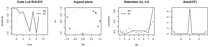
Figure 6: The best polyphase code with $R=0.974,L=9$. This code also has exceptionally high merit factor of 25.6. It is evident from the ACF, that this is nearly the most optimal code possible for a code with unit norm amplitudes, as the outermost extremes of a single pulse have to be 1. The phases in degrees are: $0,0.2,52.4,41.7,-91.1,-144.5,39.8,161.4,-25.1$.

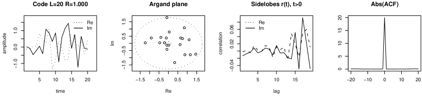
Figure 7: An amplitude and phase modulated code with amplitudes in range $a_{k}\in[0,2]$. It can be seen that the sidelobes can be reduced to nearly zero, when amplitude modulation is allowed.

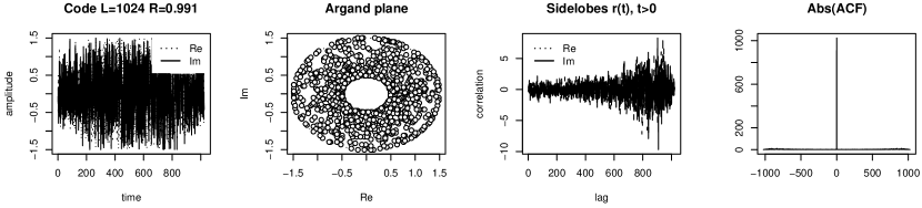
Figure 8: A long code with amplitudes in range $a_{k}\in[0.5,1.5]$.

TABLE II: Some selected codes

Length	R	Phases $\phi_{k}$ (degrees)	Amplitudes $a_{k}$
9	0.973	0 0.2 52.4 41.7 -91.1 -144.5 39.8 161.4 -25.1	1 1 1 1 1 1 1 1 1
13	1.000	98.39 -104.50 36.76 175.29 99.72 -62.70 -120.28 77.66 46.32 37.25 33.31 13.03 -21.19	0.39 1.13 1.56 1.35 0.31 1.38 0.65 1.01 1.40 1.05 0.76 0.45 0.15
20	0.988	5.46 -20.64 -40.09 -28.29 -36.87 -22.32 43.55 172.33 175.48 93.05 -34.38 -55.14 122.29 -158.74 -45.56 89.39 -79.32 136.14 -46.09 134.19	0.80 0.80 0.87 1.20 1.18 0.80 0.80 0.80 1.20 0.94 1.20 1.20 1.20 0.80 0.84 1.20 0.88 0.86 1.20 0.92
33	0.982	18.60 -100.83 161.00 33.34 -79.52 130.05 30.10 -122.23 -55.99 168.40 98.19 94.49 -77.28 4.82 -167.74 65.06 168.02 -28.00 9.50 90.79 -82.85 -3.32 -94.82 -114.72 -71.90 130.07 -169.00 -162.73 -107.41 -86.53 -48.03 -41.65 -14.85	1 1 1 1 1 1 1 1 1 1 1 1 1 1 1 1 1 1 1 1 1 1 1 1 1 1 1 1 1 1 1 1 1
42	1.000	-174.51 158.30 -126.60 139.94 -128.83 -149.15 51.30 -135.17 82.97 -31.20 139.69 -1.60 -148.26 28.75 -19.38 27.63 -21.57 35.47 143.15 -50.60 53.19 133.13 -78.68 -119.40 -72.44 103.84 72.66 40.87 -103.49 89.89 -10.03 -55.58 -170.31 93.54 -141.04 136.35 54.50 -23.15 -148.32 27.18 19.58 -125.25	0.30 0.28 0.32 0.42 0.28 0.64 0.47 0.72 0.77 0.45 0.39 1.29 0.53 1.09 1.16 1.18 1.76 1.62 0.79 1.02 1.27 1.90 1.72 1.50 1.34 1.85 1.08 1.73 1.31 0.35 1.07 0.84 0.80 0.73 0.68 0.41 0.53 0.64 0.29 0.20 0.24 0.14

X Conclusions

Estimator mean and variance was derived for matched and mismatched filter target power estimators in the case of an arbitrary target. It was seen that it is sufficient to minimize thermal noise entering the filter. It was also noted that matched filter estimator contains bias and often results in larger estimator variance than the mismatched filter when the target is distributed. The obtained equations for estimator variance can be used for more specific radar design problems where there is prior information of the range and power extent of the target.

In order to search for optimal mismatched filter estimator codes, a heuristic constrained random local improvement algorithm was used to find transmission codes that are in many cases extremely close to theoretical optimum. The width of the estimator variance is inversely proportional to $\mathrm{SNR}$ and transmission power, and thus the largest improvements in comparison to binary phase codes can be found for short transmission codes and poor $\mathrm{SNR}$ values. For good $\mathrm{SNR}$ levels and longer codes, the improvement is not as dramatic.

XI Future Work

In this study, we restricted ourselves to targets that do not have Doppler, and thus the performance of these codes in the presence of Doppler is not known. The next logical step would be to study estimation of targets with Doppler. In these cases the optimal transmission codes may be different. We only studied the performance of two natural and commonly used linear target power estimators. A more superior method would be to study target estimation as a statistical problem, selecting codes that minimize the posterior distribution of the target variable, given the measurements and prior information about the target.

XII Acknowledgements

The authors acknowledge support of the Academy of Finland through the Finnish Centre of Excellence in Inverse Problems Research.

References

- [1] Barker, R.H., Group Synchronizing of Binary Digital Systems, in Communications Theory. New York: W. Academic Press, 1953.
- [2] Nunn, C. J., Welch, L. R., Multi-Parameter Local Optimization for the Design of Superior Matched Filter Polyphase Pulse Compression Codes, IEEE International Radar Conference, May 8-12, 2000.
- [3] Turyn, R., Sequences with small correlation. In H.B. Mann (Ed.), Error correcting Codes New York: Wiley, 1976.
- [4] Lindner, J., Binary sequences up to length 40 with possible autocorrelation function. Electronics letters, 1975.
- [5] Turyn,R. J., Four-phase Barker Codes. , IEEE TRANSACTIONS ON INFORMATION THEORY, VOL, iT-20, No.3, May 1974.
- [6] Taylor, J.W. Jr., and Blinchikoff, H.J., Quadriphase code-a radar pulse compression signal with unique characteristics. , IEEE TRANSACTIONS ON AEROSPACE AND ELECTRONIC SYSTEMS, 1988.
- [7] Mow, W.H., Best quadriphase codes up to length 24 , ELECTRONICS LETTERS, Vol.29, No.10, 1993.
- [8] Key, E.L., Fowle, E.N., and Haggart, R.D., A method of sidelobe suppression in phase coded pulse compression systems. M.I.T, Lincoln Lab., Lexington, Tech. Rept., 209, 1959.
- [9] Rohling, H., Plagge, W., Mismatched-filter design for periodical binary phased signals. IEEE TRANSACTIONS ON AEROSPACE AND ELECTRONIC SYSTEMS, 1989.
- [10] Lehtinen, MS., Damtie, B., Nygrén T., Optimal binary phase codes and sidelobe-free decoding filters with application to incoherent scatter radar. Annales Geophysicae, 2004.
- [11] Damtie, B., Lehtinen, MS., Orispää M., Vierinen J., Mismatched filtering of aperiodic quadriphase codes. Submitted to IEEE Information Theory.
- [12] Lüke, H., D., Mismatched filtering of periodic quadriphase and 8-phase sequences. , IEEE TRANSACTIONS ON COMMUNICATIONS, VOL. 51, NO.7 , July 2003.