Simulation study of the interaction between large-amplitude HF radio waves and the ionosphere

Abstract

The time evolution of a large-amplitude electromagnetic (EM) wave injected vertically into the overhead ionosphere is studied numerically. The EM wave has a carrier frequency of 5 MHz and is modulated as a Gaussian pulse with a width of approximately 0.1 milliseconds and a vacuum amplitude of 1.5 V/m at 50 km. This is a fair representation of a modulated radio wave transmitted from a typical high-power HF broadcast station on the ground. The pulse is propagated through the neutral atmosphere to the critical points of the ionosphere, where the L-O and R-X modes are reflected, and back to the neutral atmosphere. We observe mode conversion of the L-O mode to electrostatic waves, as well as harmonic generation at the turning points of both the R-X and L-O modes, where their amplitudes rise to several times the original ones. The study has relevance for ionospheric interaction experiments in combination with ground-based and satellite or rocket observations.

I Introduction

Pulsed high-frequency (HF) electromagnetic (EM) waves from transmitters on the ground are regularly used for sounding the density profile and drift velocity of the overehead ionosphere [Hunsucker, 1991; Reinisch et al., 1995, Reinisch, 1996]. In 1971, it was shown theoretically by Perkins and Kaw [1971] that if the injected HF radio beams are strong enough, weak-turbulence parametric instabilities in the ionospheric plasma of the type predicted by Silin [1965] and DuBois and Goldman [1965] would be excited. Ionospheric modification experiments by a high-power HF radio wave at Platteville in Colorado [Utlaut, 1970], using ionosonde recordings and photometric measurements of artificial airglow, demonstrated the heating of electrons, the deformation in the traces on ionosonde records, the excitation of spread $F$, etc., after the HF transmitter was turned on. The triggering of weak-turbulence parametric instabilities in the ionosphere was first observed in 1970 in experiments on the interaction between powerful HF radio beams and the ionospheric plasma, conducted at Arecibo, Puerto Rico, using a scatter radar diagnostic technique [Wong and Taylor, 1971; Carlson et al., 1972]. A decade later it was found experimentally in Tromsø that, under similar experimental conditions as in Arecibo, strong, systematic, structured, wide-band secondary HF radiation escapes from the interaction region [Thidé et al., 1982]. This and other observations demonstrated that complex interactions, including weak and strong EM turbulence, [Leyser, 2001; Thidé et al., 2005] and harmonic generation [Derblom et al., 1989; Blagoveshchenskaya et al., 1998] are excited in these experiments.

Numerical simulations have become an important tool to understand the complex behavior of plasma turbulence. Examples include analytical and numerical studies of Langmuir turbulence [Robinson, 1997], and of upper-hybrid/lower-hybrid turbulence in magnetized plasmas [Goodman et al., 1994; Xi, 2004]. In this Letter, we present a full-scale simulation study of the propagation of an HF EM wave into the ionosphere, with ionospheric parameters typical for the high-latitude EISCAT Heating facility in Tromsø, Norway. To our knowledge, this is the first simulation involving realistic scale sizes of the ionosphere and the wavelength of the EM waves. Our results suggest that such simulations, which are possible with today’s computers, will become a powerful tool to study HF-induced ionospheric turbulence and secondary radiation on a quantitative level for direct comparison with experimental data.

II Mathematical Model and Numerical Setup

We use the MKS system (SI units) in the mathematical expressions throughout the manuscript, unless otherwise stated. We assume a vertically stratified ion number density profile $n_{i0}(z)$ with a constant geomagnetic field ${\bf B}_{0}$ directed obliquely to the density gradient. The EM wave is injected vertically into the ionosphere, with spatial variations only in the $z$ direction. Our simple one-dimensional model neglects the EM field $1/r$ falloff ($r$ is the distance from the transmitter), the Fresnel pattern created obliquely to the $z$ direction by the incident and reflected wave, and the the influence on the radio wave propagation due to field aligned irregularities in the ionosphere. For the EM wave, the Maxwell equations give

$$\frac{\partial{\bf B}_{1}}{\partial t}=-\widehat{\bf z}\times\frac{\partial{\bf E}}{\partial z},$$ (1)

$$\frac{\partial{\bf E}}{\partial t}=c^{2}\widehat{\bf z}\times\frac{\partial{\bf B}_{1}}{\partial z}+\frac{en_{\rm e}{\bf v}_{\rm e}}{\varepsilon_{0}},$$ (2)

where the electron fluid velocity is obtained from the momentum equation

$$\frac{\partial{\bf v}_{\rm e}}{\partial t}=-v_{{\rm e}z}\frac{\partial{\bf v}_{\rm e}}{\partial z}-\frac{e}{m_{\bf e}}[{\bf E}+{\bf v}_{\rm e}\times({\bf B}_{0}+{\bf B}_{1})]$$ (3)

and the electron density is obtained from the Poisson equation $n_{\rm e}=n_{\rm i0}(z)-({\varepsilon_{0}}/{e}){\partial E_{z}}/{\partial z}$. Here, $\widehat{\bf z}$ is the unit vector in the $z$ direction, $c$ is the speed of light in vacuum, $e$ is the magnitude of the electron charge, $\varepsilon_{0}$ is the vacuum permittivity, and $m_{\rm e}$ is the electron mass.

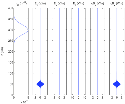
Figure 1: The ion density profile, and the electric and magnetic field components at time $t=0$ ms.

The number density profile of the immobile ions, $n_{i0}(z)=0.5\times 10^{12}\exp[-(z-300)^{2}/10^{3}]$ ($z$ in kilometers) is shown in the leftmost panel of Fig. 1. Instead of modeling a transmitting antenna via a time-dependent boundary condition at $z=0$ km, we assume that the EM pulse has reached the altitude $z=50$ km when we start our simulation, and we give the pulse as an initial condition at time $t=0$ s. In the initial condition, we use a linearly polarized EM pulse where the carrier wave has the wavelength $\lambda=60\,{\rm m}$ (wavenumber $k=0.1047\,{\rm m}^{-1}$) corresponding to a carrier frequency of $f_{0}=5\,{\rm MHz}$ ($\omega_{0}=31\times 10^{6}\,{\rm s}^{-1}$). The EM pulse is amplitude modulated in the form of a Gaussian pulse with a maximum amplitude of $1.5$ V/m, with the $x$-component of the electric field set to $E_{x}=1.5\exp[-(z-50)^{2}/10^{2}]\sin(0.1047\times 10^{3}z)$ ($z$ in kilometers) and the $y$ component of the magnetic field set to $B_{y}=E_{x}/c$ at $t=0$. The other electric and magnetic field components are set to zero; see Fig. 1. The spatial width of the pulse is approximately 30 km, corresponding to a temporal width of 0.1 milliseconds as the pulse propagates with the speed of light in the neutral atmosphere. It follows from Eq. (1) that $B_{z}$ is time-independent; hence we do not show $B_{z}$ in the figures. The geomagnetic field is set to $B_{0}=4.8\times 10^{-5}$ Tesla, corresponding to an electron cyclotron frequency of 1.4 MHz, directed downward and tilted in the $xz$-plane with an angle of $13$ degrees ($0.227$ rad) to the $z$-axis, i.e., ${\bf B}_{0}=(B_{0x},B_{0y},B_{0z})=(\sin 0.227,0,-\cos 0.227)B_{0}$. In our numerical simulation, we use $10^{5}$ spatial grid points to resolve the plasma for $0\leq z\leq 400$ km. The spatial derivatives are approximated with centered second-order difference approximations, and the time-stepping is performed with a leap-frog scheme with a time step of $\Delta t=8\times 10^{-9}$ s.

III Numerical Results

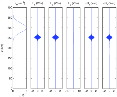
Figure 2: The ion density profile, and the electric and magnetic field components at time $t=0.720$ ms. The splitting of the wave is due to Faraday rotation.

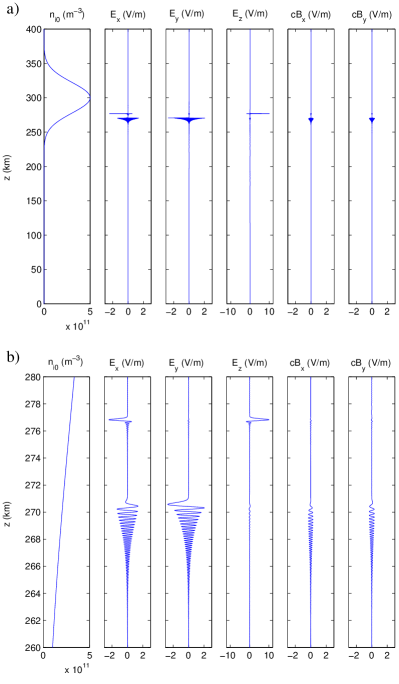
Figure 3: a) The ion density profile, and the electric and magnetic field components at time $t=0.886$ ms. b) A closeup of the region of the turning points of the R-X and L-O modes. We see that the wave-energy of the L-O mode is concentrated into one single half-wave envelop at $z\approx 277$ km, while the turning point of the less localized R-X mode is at $z\approx 270.5$ km.

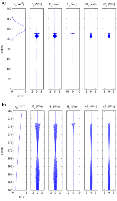
Figure 4: a) The ion density profile, and the electric and magnetic field components at time $t=0.948$ ms. b) A closeup of the region of the turning points of the R-X and L-O modes. Here, the L-O mode oscillations at $z\approx 277$ km are radiating EM waves with perpendicular (to the $z$ axis) electric field components.

In the simulation, the EM pulse propagates without changing shape through the neutral atmosphere, until it reaches the ionospheric layer. At time $t=0.720$ ms, shown in Fig. 2, the EM pulse has reached the lower part of the ionosphere. The initially linearly polarized EM wave undergoes Faraday rotation due to the different dispersion properties of the L-O and R-X modes (we have adopted the notation “L-O mode” and “R-X mode” for the two high-frequency EM modes, similarly as, e.g., Goertz and Strangeway [1995]) in the magnetized plasma, and the $E_{y}$ and $B_{x}$ components are excited. At $t=0.886$ ms, shown in Fig. 3, the L-O and R-X mode pulses are in the vicinity of their respective turning points, the turning point of the L-O mode being at a higher altitude than that of the R-X mode; see panel a) of Fig. 3. A closeup of this region, displayed in panel b), shows that the first maximum of the R-X mode is at $z\approx 270.5$ km, and the one of the L-O mode is at $z\approx 277$ km. The maximum amplitude of the R-X mode is $\approx 3$ V/m while that of the L-O mode is $\approx 10$ V/m; the latter amplitude maximum is in agreement with those obtained by Thidé and Lundborg, [1986], for a similar set of parameters as used here. The electric field components of the L-O mode, which at this stage are concentrated into a pulse with a single maximum with a width of $\approx 200$ m, are primarily directed along the geomagnetic field lines, and hence only the $E_{z}$ and $E_{x}$ components are excited, while the magnetic field components of the L-O mode are very small. At $t=0.948$ ms, shown in panel a) of Fig. 4, both the R-X and L-O mode wave packets have widened in space, and the EM wave has started turning back towards lower altitudes. In the closeup of the EM wave in panel b) of Fig. 4, one sees that the L-O mode oscillations at $z\approx 277$ km are now radiating EM waves with significant magnetic field components. Finally, shown in Fig. 5 at $t=1.752$, the EM pulse has returned to the initial location at $z=50$ km. Due to the different reflection heights of the L-O and R-X modes, the leading (lower altitude) part of the pulse is primarily R-X mode polarized while its trailing (higher altitude) part is L-O mode polarized. In the center of the pulse, where we have a superposition of the R-X and L-O mode, the wave is almost linearly polarized with the electric field along the $y$ axis and the magnetic field along the $x$ axis. The direction of the electric and magnetic fields here depends on the relative phase between the R-X and L-O mode.

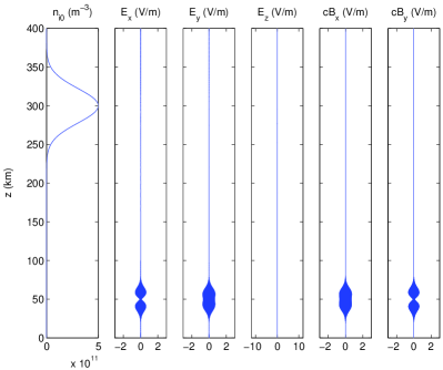
Figure 5: The ion density profile, and the electric and magnetic field components at time $t=1.752$ ms.

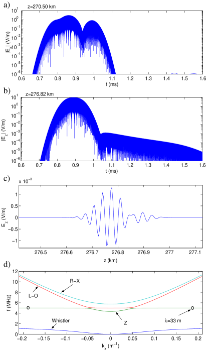
Figure 6: a) The amplitude of the electric field component $E_{x}$ at $z=270.50$ km, near the turning point of the R-X mode, and b) the amplitude of the electric field component $E_{z}$ at $z=276.82$ km, near the turning point of the L-O mode. c) A snapshot of low-amplitude electrostatic waves of wavelength $\lambda\approx 33$ m (wavenumber $k=2\pi/\lambda\approx 0.19\,{\rm m}^{-1}$), observed at time $t=1.152$ ms, and d) Dispersion curves (lower panel) obtained from the Appleton-Hartree dispersion relation with parameters $\omega_{\rm pe}=31.4\times 10^{6}\,{\rm s}^{-1}$ (5 MHz), $\omega_{\rm ce}=8.80\times 10^{6}\,{\rm s}^{-1}$ (1.4 MHz) and $\theta=13^{\circ}=0.227$ rad. We identify the high-frequency R-X and L-O modes, as well as the Z-mode which extends to the electrostatic Langmuir/Upper hybrid branch for large wavenumbers; the circles indicate the approximate locations on the dispersion curve for the electrostatic oscillations shown in panel c). For completeness we also show the low-frequency electron whistler branch in panel d).

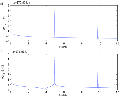
Figure 7: The frequency spectrum (10-logarithmic scale) of a) the electric field component $E_{x}$ at the altitude $z=270.50$ km, and b) of $E_{z}$ at the altitude $z=276.82$ km.

In Fig. 6, panel a), we have plotted the electric field component $E_{x}$ at $z=270.50$ km, near the turning point of the R-X mode and in panel b) we have plotted the $E_{z}$ component at $z=276.82$ km, near the turning point of the L-O mode. We see that the maximum amplitude of $E_{x}$ reaches $3$ V/m at $t=0.87$ ms, and that of $E_{z}$ reaches $10$ V/m at $t=0.9$ ms. The electric field amplitude at $z=270.50$ km has two maxima, due to the L-O mode part of the pulse, which is reflected at the higher altitude $z=276.82$ km and passes twice over the altitude $z=270.50$ km. We also observe weakly damped oscillations of $E_{z}$ at $z=276.82$ km for times $t>1.05$ ms, which decrease exponentially in time between $t=1.1$ ms and $t=1.5$ ms as $E_{z}\propto\exp(-\gamma t)$ with $\gamma=6.5\times 10^{3}$ s^-1. We found from the numerical values that $\gamma\approx ck_{n}/2$, where $k_{n}=d{\rm ln}n_{i0}/dz\approx 4.6\times 10^{-5}\,{\rm m}^{-1}$ is the inverse ion density scale length at $z=277$ km, but we are not certain how general this result is. No detectable magnetic field fluctuations are associated with these weakly damped oscillations, and we interpret them as electrostatic waves that have been produced by mode conversion of the L-O mode. The amplitudes of the $E_{x}$ and $E_{y}$ components are also much weaker than that of the $E_{z}$ component for these oscillations. A closeup of these electrostatic oscillations at $t=1.152$ ms is displayed in panel c) of Fig. 6, where we see that they have a wavelength of approximately 33 m (wavenumber $0.19\,{\rm m}^{-1}$). In panel d) of Fig. 6, we have plotted the frequency $f=\omega/2\pi$ as a function of the wavenumber $k$, where $\omega$ is obtained from the Appleton-Hartree dispersion relation [Stix, 1992]

$$\omega^{2}=c^{2}k_{z}^{2}+\frac{2\omega_{\rm pe}^{2}(\omega^{2}-\omega_{\rm pe}^{2})}{2(\omega^{2}-\omega_{\rm pe}^{2})-\omega_{\rm ce}^{2}\sin^{2}\theta\pm\omega_{\rm ce}\Delta}.$$ (4)

Here $\Delta=[\omega_{\rm ce}^{2}\sin^{4}\theta+4\omega^{-2}(\omega^{2}-\omega_{\rm pe}^{2})^{2}\cos^{2}\theta]^{1/2}$, $\omega_{\rm pe}$ ($\omega_{\rm ce}$) is the electron plasma (cyclotron) frequency, and $\theta$ is the angle between the geomagnetic field and the wave vector ${\bf k}$, which in our case is directed along the $z$-axis, ${\bf k}=k_{z}\widehat{\bf z}$. We use $\omega_{\rm pe}=31.4\times 10^{6}\,{\rm s}^{-1}$ (corresponding to $f_{\rm pe}=5$ MHz), $\omega_{\rm ce}=8.80\times 10^{6}\,{\rm s}^{-1}$ (corresponding to $f_{\rm ce}=1.4$ MHz) and $\theta=13^{\circ}=0.227$ rad. The location of the electrostatic waves whose wavelength is approximately 33 m and frequency 5 MHz is indicated with circles in the diagram; they are on the same dispersion surface as the Langmuir waves and the upper hybrid waves/slow Z mode waves with propagation parallel and perpendicular to the geomagnetic field lines, respectively. The mode conversion of the L-O mode into electrostatic oscillations are relatively weak in our simulation of vertically incident EM waves, and theory shows that the most efficient linear mode conversion of the L-O mode occurs at two angles of incidence in the magnetic meridian plane, given by, e.g., Eq. (17) in [Mjølhus, 1990].

The nonlinear effects at the turning point of the L-O and R-X modes are investigated in Fig. 7 which displays the frequency spectrum of the electric field component $E_{x}$ at the altitude $z=270.5$ km and of $E_{z}$ at the altitude $z=276.82$ km. The spectrum shows the large-amplitude pump wave at 5 MHz and the relatively weak second harmonics of the pump wave at 10 MHz at both altitudes (the slight downshift is due to numerical errors produced by the difference approximations used in space and time). Visible are also low-frequency oscillations (zeroth harmonic) due to the nonlinear down-shifting/mixing of the high-frequency wave field.

IV Summary

In conclusion, we have presented a full-scale numerical study of the propagation of an EM wave and its linear and nonlinear interactions with an ionospheric layer. We observe the reflection of the L-O and R-X modes at different altitudes, the mode conversion of the L-O mode into electrostatic Langmuir/upper hybrid waves as well as nonlinear harmonic generation of the high-frequency waves. Second harmonic generation have been observed in ionospheric heating experiments [Derblom et al., 1989; Blagoveshchenskaya et al., 1998] and may be partially explained by the cold plasma model presented here.

Acknowledgment This work was supported financially by the Swedish Research Council (VR).

References

- Blagoveshchenskaya et al., (1998) Blagoveshchenskaya, N. F., V. A. Kornienko, M. T. Rietveld, B. Thidé, A. Brekke, I. V. Moskvin, and S. Nozdrachev (1998), Stimulated emissions around second harmonic of Tromsø heater frequency observed by long-distance diagnostic HF tools. Geophys. Res. Lett., 25(6), 863–876.
- Carlson et al., (1972) Carlson, H. C., W. E. Gordon, and R. L. Showen (1972), HF induced enhancements of incoherent scatter spectrum at Arecibo, J. Geophys. Res., 77, 1242–1250.
- Derblom et al., (1989) Derblom, H., B. Thidé, T. B. Leyser, J. A. Nordling, Å. Hedberg, P. Stubbe, H. Kopka, and M. Rietveld (1989), Tromsø heating experiments: stimulated emission at HF pump harmonic and subharmonic frequencies, J. Geophys. Res. 94(A8), 10111–10120.
- DuBois and Goldman, (1965) DuBois, D. F. and M. V. Goldman (1965), Radiation-induced instability of electron plasma oscillations, Phys. Rev. Lett., 14, 544–546.
- Goertz and Strangeway, (1995) Goertz, C. K., and R. J. Strangeway (1995), Plasma waves, in Introduction to Space Physics, edited by M. G. Kivelson and C. T. Russell, pp. 356-399, Cambridge University Press, New York.
- Goodman et al., (1994) Goodman, S., H. Usui, and H. Matsumoto (1994), Particle-in-cell (PIC) simulations of electromagnetic emissions from plasma turbulence, Phys. Plasmas 1, 1765–1767.
- Hunsucker, (1991) Hunsucker, R. D. (Ed.) (1991), Radio techniques for probing the terrestrial ionosphere, 293 pp., Springer, Berlin.
- Leyser, (2001) Leyser, T. B. (2001), Stimulated electromagnetic emissions by high-frequency electromagnetic pumping of the ionospheric plasma, Space Sci. Rev. 98, 223–328.
- Mjølhus, (1990) Mjølhus, E. (1990), On linear conversion in a magnetized plasma, Radio Sci. 25(6), 1321–1339.
- Perkins and Kaw, (1971) Perkins, F. W. and P. K. Kaw (1971), On the role of plasma instabilities in ionospheric heating by radio waves, J. Geophys. Res. 76, 282–284.
- Reinisch et al., (1995) Reinisch, B. W., T. W. Bullett, J. L. Scali, and D. M. Haines (1995), High latitude digisonde measurements and their relevance to IRI, Adv. Space Res. 16(1), (1)17–(1)26.
- Reinisch, (1996) Reinisch, B. W. (1996), Modern Ionosondes, in Modern Ionospheric Science, edited by H. Kohl, R. Ruster and K. Schlegel, pp. 440-458, EGS, Katlenburg-Lindau, Germany.
- Robinson, (1997) Robinson, P. A. (1997), Nonlinear wave collapse and strong turbulence, Rev. Mod. Phys. 69, 507–574.
- Silin, (1965) Silin, V. P. (1965), Parametric resonance in plasma, Sov. Phys. JETP, 21, 1127–1134.
- Stix, (1992) Stix, H. (1992), Waves in Plasmas, Springer-Verlag, New York.
- Thidé et al., (1982) Thidé, B., H. Kopka, and P. Stubbe (1982), Observations of stimulated scattering of a strong high-frequency radio wave in the ionosphere, Phys. Rev. Lett. 49, 1561.
- Thidé and Lundborg, (1986) Thidé, B., and B. Lundborg (1986), Structure of HF pump in ionospheric modification experiments. Linear treatment, Phys. Scr. 33, 475–479.
- Thidé et al., (2005) Thidé, B., E. N. Sergeev, S. M. Grach, T. B. Leyser, and T. D. Carozzi (2005), Competition between Langmuir and upper-hybrid turbulence in a high-frequency-pumped ionosphere, Phys. Rev. Lett. 95, 255002.
- Utlaut, (1970) Utlaut, W. F. (1970), An ionospheric modification experiment using very high power, high frequency transmission, J. Geophys. Res., 75(31), 6402-6405.
- Wong et al., (1971) Wong, A. Y. and R. J. Taylor (1971), Parametric excitation in the ionosphere, Phys. Rev. Lett., 27, 644–647.
- Xi, (2004) Xi, H. (2004), Theoretical and Numerical Studies of Frequency Up-shifted Ionospheric Stimulated Radiation PhD Thesis, Virginia Polytechnic Institute and State University, etd-10152004-191708.