The X${}^{1}\Sigma^{+}$ and a${}^{3}\Sigma^{+}$ states of LiCs studied by Fourier-transform spectroscopy

Abstract

We present the first high-resolution spectroscopic study of LiCs. LiCs is formed in a heat pipe oven and studied via laser-induced fluorescence Fourier-transform spectroscopy. By exciting molecules through the X${}^{1}\Sigma^{+}$-B${}^{1}\Pi$ and X${}^{1}\Sigma^{+}$-D${}^{1}\Pi$ transitions vibrational levels of the X${}^{1}\Sigma^{+}$ ground state have been observed up to 3 $\,\rm cm^{-1}$ below the dissociation limit enabling an accurate construction of the potential. Furthermore, rovibrational levels in the a${}^{3}\Sigma^{+}$ triplet ground state have been observed because the excited states obtain sufficient triplet character at the corresponding excited atomic asymptote. With the help of coupled channels calculations accurate singlet and triplet ground state potentials were derived reaching the atomic ground state asymptote and allowing first predictions of cold collision properties of Li + Cs pairs.

I Introduction

Spectroscopy of heteronuclear diatomic alkali molecules provides important input to current research in cold molecules and mixtures of ultracold atomic gases. Cold heteronuclear alkali dimers are subject to a large interest since they can be formed at temperatures below 1$\,\rm mK$ Kraft et al. (2006); Mancini et al. (2004); Wang et al. (2004); Haimberger et al. (2004); Kerman et al. (2004) and possess a large permanent electric dipole moment for deeply bound singlet levels Aymar and Dulieu (2005); Igel-Mann et al. (1986). This combination of properties enables electric field control of ultracold collisions Krems (2005, 2006) and cold chemical reactions Balakrishnan and Dalgarno (2001); Bodo et al. (2002) and holds promises for applications in quantum computation DeMille (2002). Precise potential energy curves, in particular for the lowest electronic states, are evidently important for such applications as well as for understanding the molecule formation processes (photoassociation), ro-vibrational state selective detection Kerman et al. (2004); Wang et al. (2005) and for formation of vibrational ground-state molecules Sage et al. (2005). In ultracold mixtures of atomic gases, quantum degeneracy of one atomic species can be achieved through sympathetic cooling by the other species DeMarco and Jin (1999); Modugno et al. (2001); Truscott et al. (2001). The interspecies interaction strength can be varied through magnetic Feshbach resonances and has a large influence on a variety of effects such as phase-separation between a Bose-Einstein condensate and a degenerate Fermi gas  Mølmer (1998) and the transition to a Bardeen-Cooper-Schrieffer superfluid state in dilute Fermi gases Heiselberg et al. (2000). Understanding interspecies collision properties at the atomic ground state asymptotes, e.g. predicting the magnetic field strength values of Feshbach resonances at zero kinetic energy, requires precise potential curves of the electronic ground states.

Cold LiCs molecules were observed very recently, being formed in a two-species magneto-optical trap Kraft et al. (2006). Previously, inelastic collisions Schlöder et al. (1999) and sympathetic cooling of Li by Cs in an optical dipole trap Mudrich et al. (2002) have been studied. Recent theoretical work considers LiCs in strong dc electric fields and its influence on rovibrational dynamics Gonzalez-Ferez et al. (2006) and Li-Cs collision cross sections Krems (2006).

Although LiCs was observed already in 1928 by Walter and Barratt through absorption in a mixture of metallic vapors Walter and Barratt (1928), very few and no high-resolution spectroscopic studies have been made until now. In the 1980’s Vadla et al. studied the repulsive Li(2p)+Cs(6s) asymptote Vadla et al. (1983). More recently LiCs molecules were formed on He nanodroplets and excitation spectra of the d${}^{3}\Pi\leftarrow$ a${}^{3}\Sigma^{+}$ transition were recorded and modeled Mudrich et al. (2004). Ab initio potentials were calculated by Korek et al. Korek et al. (2000) (see Fig. 1) and more recently an extended theoretical study was done by Aymar and Dulieu Aymar and Dulieu (2005). The theoretical potentials provide a good starting point for analysis of the spectra obtained in the present work.

Here we present a high-resolution spectroscopic study of the LiCs molecule. Similar to our previous studies Pashov et al. (2005); Docenko et al. (2006) we apply Fourier-transform spectroscopy of laser-induced fluorescence from LiCs molecules formed in a heat-pipe, because this technique is suitable for collecting a large amount of accurate experimental data. By using properly chosen excitation schemes (see e.g. Pashov et al. (2005); Docenko et al. (2006)) we can measure transition frequencies to a wide range of vibrational levels in the singlet X${}^{1}\Sigma^{+}$ as well as in the triplet a${}^{3}\Sigma^{+}$ ground states, especially levels close to the asymptote. Since the two states are coupled at long internuclear distances by the hyperfine interaction it is not correct to treat them separately in this region, as it would lead to model potentials which are unable to reproduce the experimental observations close to the asymptote. Therefore, the aim of our experimental work is to collect experimental data on both ground states and to fit accurate experimental potential energy curves simultaneously for both states - the indispensable starting point for a study of the molecular structure of LiCs or for modeling of cold collision processes on the Li(2s)+Cs(6s) asymptote. We apply these potential curves within a coupled channels model in order to explain our experimental observations and also to compute collision properties for comparing recent results of sympathetic cooling of Li by Cs Mudrich et al. (2002)

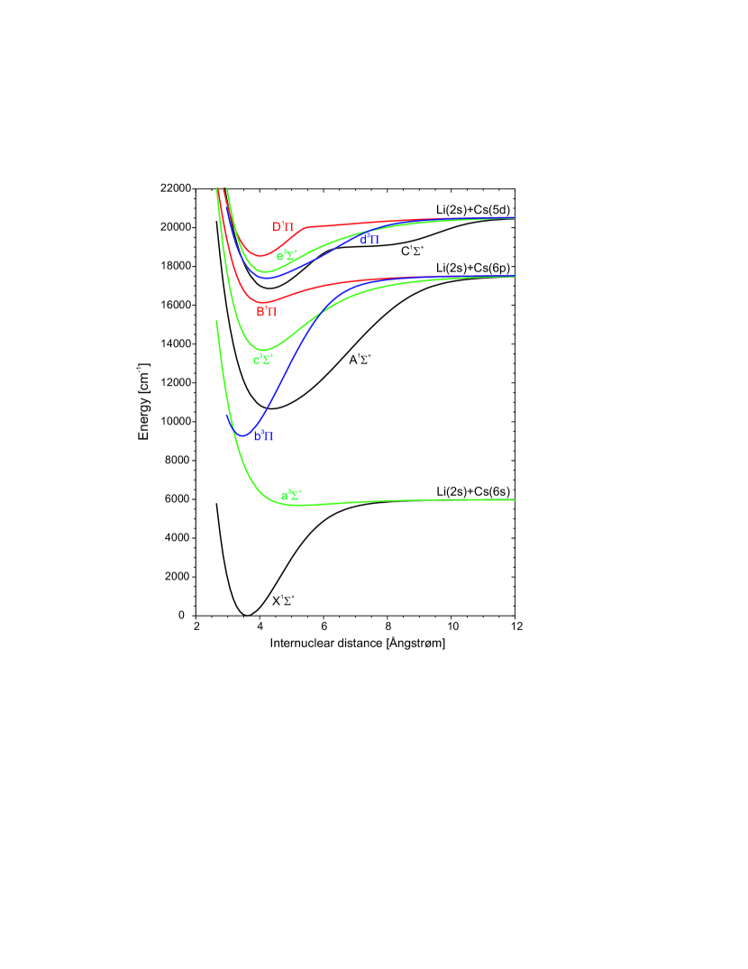
Figure 1: (Color online) Selected singlet and triplet potential energy curves in LiCs Korek et al. (2000).

The article is organized as follows: The experimental setup and excitation schemes are presented in Section II. In Section III we describe the analysis of the obtained spectra. The procedure for construction of potential energy curves is described in Section IV and the potentials are reported. In Section V we give our conclusion and an outlook for further experimental study needed for a quantitative description of ultracold collisions in Li + Cs.

II Experiment: molecule formation and spectroscopy

II.1 Molecule formation

LiCs molecules are formed in a stainless steel heat-pipe identical to the one described in Ref. Docenko et al. (2004), except for one modification described below. The heat-pipe (960$\,\rm mm$ long and 34$\,\rm mm$ outer diameter) is filled with 6$\,\rm g$ Li and 5$\,\rm g$ Cs (the Cs, in a closed ampoule, is loaded into the side container Docenko et al. (2004) ) and typically operated with 3-6 $\,\rm mbar$ Ar buffer gas pressure.

Since the vapor pressure difference between Li and Cs at a common temperature is extremely large, we modified the design of Ref. Docenko et al. (2004) in order to obtain a three-section heat-pipe, which is more suitable for producing a vapor mixture with similar concentrations of Li and Cs and hence for forming LiCs molecules Bednarska et al. (1996). In Ref. Docenko et al. (2004) the central 60$\,\rm cm$ of the heat-pipe is heated uniformly in a commercial oven (Carbolite); here we mount two stainless steel ’shells’ (20$\,\rm cm$ long, 50$\,\rm mm$ inner diameter) concentrically around the heat-pipe and seal up the ends facing towards the center of the oven such that only the central 20$\,\rm cm$ of the heat-pipe are heated directly in the oven. By blowing air into the open ends, which extend outside of the oven, we can maintain a lower temperature in the sections shielded by the shells than in the central part of the heat-pipe.

The heat-pipe is conditioned by heating it to temperatures of about 580$\,\rm{}^{\circ}C$ under 10$\,\rm mbar$ Ar pressure; subsequently the Cs ampoule is broken by shaking the tube. Operating temperatures are 540$\,\rm{}^{\circ}C$ in the central part and 370$\,\rm{}^{\circ}C$ in the outer sections. The heat-pipe oven was operated for more than 200 hours over a 10 month period and was still in good working conditions at the end of this period.

II.2 Laser-induced fluorescence Fourier-transform spectroscopy

Laser-induced fluorescence from LiCs molecules is observed after excitation on the B${}^{1}\Pi\leftarrow$ X${}^{1}\Sigma^{+}$ and D${}^{1}\Pi\leftarrow$ X${}^{1}\Sigma^{+}$ transitions. The B${}^{1}\Pi\leftarrow$ X${}^{1}\Sigma^{+}$ transitions were excited using a Coherent 599 dye laser (with DCM dye) at frequencies in the range 15529-16123$\,\rm cm^{-1}$ and a Coherent 699 dye laser at frequencies in the range 16397-17022$\,\rm cm^{-1}$ (with Rhodamine 6G dye as well as with a mixture of Rhodamine 6G and Rhodamine B). The D${}^{1}\Pi\leftarrow$ X${}^{1}\Sigma^{+}$ transition was excited using the dye laser with Rhodamine 6G at frequencies in the range 16663-17238$\,\rm cm^{-1}$ and a frequency doubled Nd:YAG laser. The strongest signals were observed for the B${}^{1}\Pi\leftarrow$ X${}^{1}\Sigma^{+}$ system and we studied the ground states mainly through this system. We note that indeed Walter and Barratt observed strong absorption in the range 15983-16582$\,\rm cm^{-1}$ Walter and Barratt (1928) which according to Fig. 1 corresponds to the B${}^{1}\Pi\leftarrow$ X${}^{1}\Sigma^{+}$ transition. At excitation frequencies in the range $\sim 14900-15400$$\,\rm cm^{-1}$, we find strong fluorescence due to Li₂ and NaCs (Na is present as an impurity in the Li sample) which overshadows a possible LiCs signal. Using an Ar-ion laser for excitation at 457.9$\,\rm nm$, 476.5$\,\rm nm$, 488.0$\,\rm nm$, 496.5$\,\rm nm$ and 514.5$\,\rm nm$ we did not observe any fluorescence from LiCs molecules, only from Li₂, LiNa and NaCs.

Contrary to the previously studied molecules NaRb Pashov et al. (2005) and NaCs Docenko et al. (2006), the low lying levels of the excited B${}^{1}\Pi$ state in LiCs turned out to be almost free of local perturbations by the neighboring triplet states b${}^{3}\Pi$ and c${}^{3}\Sigma^{+}$, which could be expected from the theoretical potential curves (see Fig. 1). As a consequence we were unable to register any transition to the triplet ground state from the low lying B${}^{1}\Pi$ state levels. We searched instead for access to the triplet manifold through local perturbations in the D${}^{1}\Pi$ and C${}^{1}\Sigma^{+}$ states. Here we used a Coumarine 6 dye laser with a typical power of 25 mW. Unfortunately within the searched excitation frequency region of 18446 - 19039 cm^-1 we were also not able to register transitions to the triplet ground state.

The only fluorescence to the a${}^{3}\Sigma^{+}$ state is observed after excitation to high lying levels in the B${}^{1}\Pi$ state. These transitions are attributed to the long-range change over of coupling case for the B${}^{1}\Pi$ state itself rather than to local mixing of the B${}^{1}\Pi$ state at long range with the neighboring triplet states Pashov et al. (2005); Docenko et al. (2006). This conclusion is supported first, by the observation that high lying B state levels seem to be locally unperturbed. Second, the intensity distribution of progressions from the high lying B state levels to the ground singlet state could be explained satisfactory by the Franck-Condon factors between the X and the B states, including the highest $v_{X}^{\prime\prime}$ levels (contrary to the case of NaRb Pashov et al. (2005)). So transitions from these B state levels to high lying a${}^{3}\Sigma^{+}$ state levels will become also probable when the B state changes its character from Hund’s case (a) ${}^{1}\Pi$ to Hund’s case (c) $\Omega=1$ at long internuclear distances. Indeed, in our spectra we find transitions mainly to high $v_{a}^{\prime\prime}$ and none to the bottom of the triplet ground state.

The laser-induced fluorescence light is collected in the direction opposite to the one of laser beam propagation and recorded by a Bruker IFS 120HR Fourier-Transform Spectrometer (FTS). For detection we use a photomultiplier (Hamamatsu R928) or a Si-photodiode. In order to avoid illumination of the detector by the He-Ne laser (632.8 nm), used in the FTS for calibration and stepping control, a notch filter (8$\,\rm nm$ full width at half maximum) is introduced in the beam path, which suppresses also the fluorescence induced in the corresponding spectral region. The resolution of the FTS is typically set to 0.03 - 0.05 $\,\rm cm^{-1}$. The uncertainty of the line positions is estimated to be $1/10$ of the resolution. For lines with signal-to-noise ratio less than 3 the uncertainty is gradually increased. Each spectrum results typically from an average of 10-20 scans, but the number of scans is varied from 5 to 350 depending on the signal strength for the features of interest in the spectra. For improving the signal-to-noise ratio, the spectral window for some spectra is limited by using color glass filters or interference filters. In order to facilitate the identification in such cases we recorded also a spectrum at the same excitation frequency without filters, but with lower resolution (0.1 cm^-1) and a smaller number of scans.

A list of all excitation frequencies used in these experiments together with the assignment of the excitation transitions are given in Tables 3 and 4 of the supplementary materials EPA .

III Analysis of spectra

III.1 The X${}^{1}\Sigma^{+}$ state

Assignment of the large number of transitions, about 6600, to the X${}^{1}\Sigma^{+}$ state is done in an iterative process; by gradually improving the potential for the X${}^{1}\Sigma^{+}$ state, more and more transitions can be correctly assigned.

Initially, we identify several strong doublet series which are clearly recognized as P-R components from the regular development of the doublet spacing. Among these series we choose those with similar spacing, i.e., with similar rotational quantum numbers. Based on the theoretical potential for the X${}^{1}\Sigma^{+}$ state Korek et al. (2000) we make an initial guess for the vibrational and the rotational quantum numbers of these fluorescence progressions. The quantum numbers that give the closest agreement with the theoretical vibrational and rotational spacings are assigned and a small set of Dunham coefficients is fitted. If the fit is successful we can use the fitted coefficients to assign new progressions; if not, a reassignment of the quantum numbers must be made. After some iterations we obtain a self consistent set of assigned experimental progressions which can be satisfactory described by a few Dunham coefficients. This is a first hint of a correct rotational numbering. Here we point out the very good quality of the theoretical calculations Korek et al. (2000); Aymar and Dulieu (2005); the theoretical rotational numbering needed a correction by only two or three units.

When the list of assigned transitions reaches several hundreds we perform the first potential fits. Initially, we start with a pointwise potential (defined in Section IV) based on the theoretical curve Korek et al. (2000) and improve it using the procedure described in Ref. Pashov et al. (2000). In the further analysis of the spectra we apply this pointwise potential curve since outside the range of the fitted $v^{\prime\prime}$ and $J^{\prime\prime}$, it usually possesses better predictive properties than the Dunham type coefficients. Moreover our experience from previous studies Docenko et al. (2004); Pashov et al. (2005) shows that a potential curve which fits long vibrational progressions recorded at high precision in a wide range of rotational quantum numbers indicates the correctness also of the vibrational numbering.

Finally, the established vibrational numbering was confirmed by assigning several progressions for the less abundant ⁶Li¹³³Cs molecule. These progressions fit to the experimental potential based only on ⁷Li¹³³Cs data when the appropriate reduced mass is applied Audi et al. (2003).

In order to describe the important long-range part of the potential, it is of great value to collect data with transitions to high-lying levels of the ground state. Since we noticed during the measurements that transitions to such high-lying levels originate from high-lying vibrational levels of the B${}^{1}\Pi$ state, we studied this state in order to optimize the experimental conditions for observation of near asymptotic levels in the X${}^{1}\Sigma^{+}$ state (a report on the B${}^{1}\Pi$ state is in preparation Pashov et al. (2006)). From the available experimental term energies of the B${}^{1}\Pi$ state levels a preliminary potential for the B${}^{1}\Pi$ state was fitted. This potential was then used to predict transition frequencies for excitation transitions with large Franck-Condon factors. In this way we recorded systematically transitions from $v^{\prime}=24$ and 25 to the X${}^{1}\Sigma^{+}$ state for a wide range of $J^{\prime}$, thus adding several ro-vibrational levels with $v_{X}^{\prime\prime}=49$ and 50 to the ground state dataset. In most cases such high-lying levels of the X${}^{1}\Sigma^{+}$ state could be observed with a sufficient signal-to-noise ratio only by increasing the number of summed scans to several hundreds. We searched for excitations to higher vibrational levels of the B${}^{1}\Pi$ state within predicted spectral regions but we were not able to register fluorescence from $v^{\prime}\geq 26$ to the X${}^{1}\Sigma^{+}$ state, most likely due to possible predissociation or unfavorable transition probabilities.

III.2 The a${}^{3}\Sigma^{+}$ state

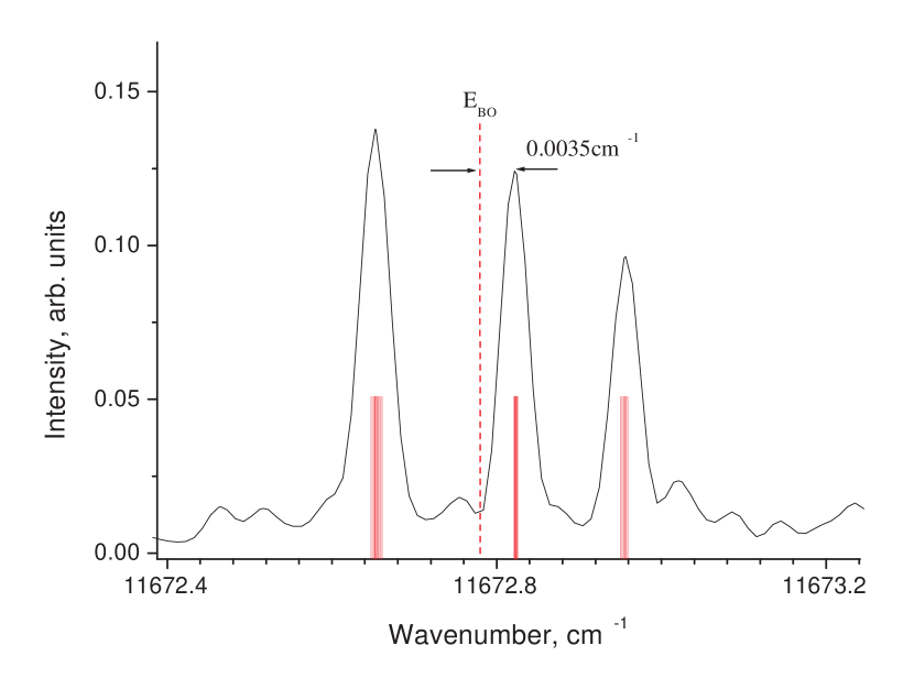
Figure 2: (Color online) Hyperfine structure of a transition to the $v_{a}^{\prime\prime}=9$, $N_{a}^{\prime\prime}=17$ level of the a${}^{3}\Sigma^{+}$ state. The vertical full lines indicate the prediction of the coupled channels calculation. The dashed vertical line indicates the position of the hyperfine-structure free level, which is shifted by 0.035 cm^-1 from the central component of the structure.

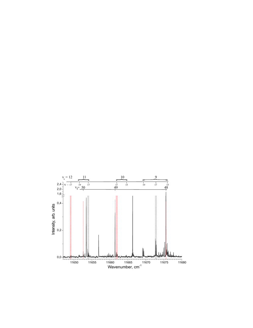
Figure 3: (Color online) Portion of recorded progression from the B state level with $v^{\prime}=25$, $J^{\prime}=17$ excited by a Q-type transition. Lines not marked on the figure belong to another assigned progression.

The triplet transitions are easily distinguished by their hyperfine structure (HFS) which at our resolution consists of three lines split by approximately 0.3 cm^-1. Calculations similar to those in Ref. Kasahara et al. (1996) show that the observed splitting is well reproduced by the Fermi contact interaction model applying the atomic HFS constants for ⁷Li and ¹³³Cs Arimondo et al. (1977). In Fig. 2 a transition to the triplet state level $v^{\prime\prime}_{a}=9,N_{a}^{\prime\prime}=17$ is shown together with the prediction of the splitting modeled by a coupled channels calculation as described in Section IV. A larger portion of the same progression originating from the $v^{\prime}=25$, $J^{\prime}=17$ B${}^{1}\Pi$ state level excited by a Q-type ($\Delta J=0$) transition is shown in Fig. 3. Some of the transitions reach near asymptotic levels in both ground states. The vertical dashed lines indicate the prediction of the coupled channels calculation for $J^{\prime\prime}=N^{\prime\prime}=17$ in which the hyperfine interaction between the states is included. The progression to the X${}^{1}\Sigma^{+}$ state is formed by Q-lines whereas the progression to the a${}^{3}\Sigma^{+}$ state consists of transitions to $N_{a}^{\prime\prime}=$15, 17 and 19. Lines not marked in the figure belong to another progression also assigned and used in our analysis.

The rotational assignment of the triplet lines is straightforward since we always find the progression to the X${}^{1}\Sigma^{+}$ state which shares the excited level in the B${}^{1}\Pi$ state with the progression to the a${}^{3}\Sigma^{+}$ state. The vibrational assignment of the transitions to the triplet ground state is done in the same way as for the X${}^{1}\Sigma^{+}$ state, however, no transitions in ⁶Li¹³³Cs were observed and hence the vibrational assignment relies only on the internal consistency of the total procedure.

III.3 Data sets

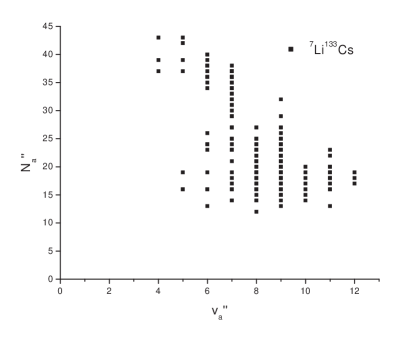
Figure 4: (Color online) Observed ro-vibrational levels in the X${}^{1}\Sigma^{+}$ and a${}^{3}\Sigma^{+}$ states of ⁷Li¹³³Cs and ⁶Li¹³³Cs.

Altogether about 6600 transitions to the X${}^{1}\Sigma^{+}$ state (130 of them belong to ⁶Li¹³³Cs) and 180 transitions to the a${}^{3}\Sigma^{+}$ state in ⁷Li¹³³Cs were assigned (see Tables 1 and 2 of the supplementary materials EPA ). The corresponding distribution of vibrational and rotational quantum numbers is shown in Figure 4. For the X${}^{1}\Sigma^{+}$ state we observe transitions to $v_{X}^{\prime\prime}=0-50$ in ⁷Li¹³³Cs. The set of a${}^{3}\Sigma^{+}$ state vibrational levels covers $v_{a}^{\prime\prime}=4-12$ and the vibrational numbering established in this study agrees with that from the theoretical potential. The limited number of experimental data, however, might lead to a revision of this assignment in the future, if additional data on the a${}^{3}\Sigma^{+}$ state are collected. Although the data set for the a${}^{3}\Sigma^{+}$ state may seem fragmentary compared to our similar studies in other molecules, the collection of these data is extremely valuable, first, due to the limited possibilities for exciting triplet states in LiCs and, second, since a proper description of the Li(2s)+Cs(6s) asymptote is only possible if both the X${}^{1}\Sigma^{+}$ state and a${}^{3}\Sigma^{+}$ state are treated in a coupled channels manner as described in the next section.

IV Construction of potential energy curves

The self-consistent assignment and fitting procedure described above gives rise to accurate pointwise short-range potentials Pashov et al. (2000). For the long-range part of both potentials we use an extension of the form

$$U_{\mathrm{LR}}(R)=U_{\infty}-\frac{C_{6}}{R^{6}}-\frac{C_{8}}{R^{8}}-\frac{C_{10}}{R^{10}}\pm E_{ex}\mbox{ .}$$ (1)

Here $U_{\infty}$ is the energy of the atomic asymptote with respect to the minimum of the X${}^{1}\Sigma^{+}$ state potential, $C_{6}$, $C_{8}$ and $C_{10}$ are the dispersion coefficients and

$$E_{ex}(R)=A_{ex}\cdot R^{\gamma}\cdot e^{-\beta R}$$ (2)

is the frequently applied functional form of the exchange energy B.M.Smirnov and M.I.Chibisov (1965) which is added for the triplet state and subtracted for the singlet state.

The pointwise short-range and the long-range potentials are connected at a point $R_{o}$ ensuring a smooth transition between both potential branches. $R_{o}$ is chosen as described in Refs. Allard et al. (2002); Pashov et al. (2005), the $C_{6}$ and $C_{8}$ coefficients are fixed to their theoretical values Marinescu and Sadeghpour (1999); Derevianko et al. (2001); Porsev and Derevianko (2003), $\gamma$ and $\beta$ are estimated using the ionization potentials for Li and Cs Radzig and Smirnov (1985) according to Ref. B.M.Smirnov and M.I.Chibisov (1965), while $U_{\infty}$, $C_{10}$ and A_ex are adjusted during the fitting procedure.

In the first step of the fitting procedure we adjust only the pointwise part of the potential for the X${}^{1}\Sigma^{+}$ state. The experimental transition frequencies are fitted by adjusting the parameters of the pointwise potential and the term energies of the excited levels.

As we choose the origin of the potential energy at the minimum of the X${}^{1}\Sigma^{+}$ state potential, in the second step of the fitting procedure we need to determine the term energies of the a${}^{3}\Sigma^{+}$ state levels with respect to the X${}^{1}\Sigma^{+}$ state. We do this using spectra where we observe simultaneously progressions to the singlet and the triplet states originating from a common upper state level. For a given singlet ground state potential we calculate the term energies of the triplet state using the energy of the excited level, determined in the previous step, and the progression to the a${}^{3}\Sigma^{+}$ state from this level. These a${}^{3}\Sigma^{+}$ term energies are then used in order to fit the potential parameters of the triplet state. In this way we ensure always a proper position of the a${}^{3}\Sigma^{+}$ state with respect to the X${}^{1}\Sigma^{+}$ state.

In order to treat the hyperfine structure of the spectral lines of the triplet state we checked the experimental data that the splitting within our resolution is independent of the vibrational and rotational quantum numbers $v^{\prime\prime}$ and $N^{\prime\prime}$ (except for very few cases, which we discuss below). Therefore, we use the central component of the structure for identification of the transition (see Fig. 2). We convert the observed frequency to term energy, and take into account the shift (-0.035 cm^-1, which means the hyperfine level is more deeply bound than the unperturbed level) of the selected hyperfine component from the unperturbed, hyperfine structure free one, thus we fit with the constructed term values a Born-Oppenheimer potential.

For high vibrational levels, and especially in cases of close approach of singlet and triplet levels with the same rotational quantum numbers, significant deviations from the Born-Oppenheimer picture can be expected Pashov et al. (2005); Docenko et al. (2006). In ⁷Li¹³³Cs this is most pronounced for $v_{X}^{\prime\prime}=49$ in the singlet and $v_{a}^{\prime\prime}=10$ in the triplet state (see Fig. 3). The deviations of the transitions determined by the Born-Oppenheimer potentials (indicated with thick blue bars in Fig. 5) from the experimental ones are significant and reach 0.06 cm^-1 for $v_{X}^{\prime\prime}=49$ and $J^{\prime}=24$. Fig. 5 shows the development from low $J$ to high $J$.

Therefore, in a third step, the Born-Oppenheimer potentials are refined by extending the single channel approach from the first two steps and applying a coupled channels calculation as discussed in detail in Refs. Pashov et al. (2005); Docenko et al. (2006). Briefly, we calculate the difference between the single channel and coupled channels eigenvalues and subtract these differences from the experimentally observed transition frequencies in order to obtain the frequencies which would be observed without hyperfine coupling between the singlet and the triplet ground states. Next, these frequencies are used in a combined fit to adjust the parameters of the long-range extensions of the potentials as well as in separate fits (described for the first two steps) of the short range pointwise part of the triplet and singlet potentials. Finally, the whole fitting procedure is repeated until the frequencies predicted with the coupled channels calculations agree with the experimental observations. The importance of the coupled channels calculation is illustrated in Fig. 5, where the predictions for the coupled system are shown with thin red bars together with the experimentally observed lines and the single channel predictions (thick blue bars). The degree of mixing between the triplet and singlet levels is characterized by the expectation value of the total spin operator $\left|\bm{S}\right|$ which is indicated for each line in Fig. 5.

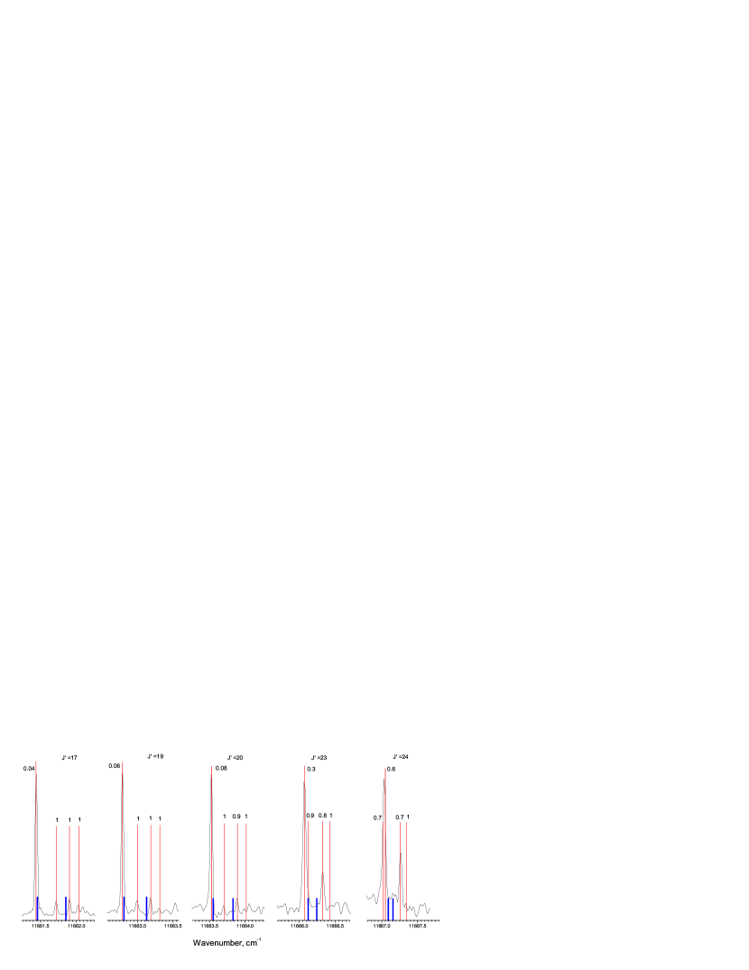
Figure 5: (Color online) Observed transitions to $v_{X}^{\prime\prime}=49$ and $v_{a}^{\prime\prime}=10$ for different $J^{\prime}$ as indicated on the figure and excited by a Q-type transition. An extended portion of the spectrum for $J^{\prime}=17$ for several $v_{a}^{\prime\prime}$ is shown in Fig. 3. For increasing $J^{\prime}$ the singlet and triplet lines approach each other, resulting in strong perturbations of the line structure and the intensity distribution within the HFS of the triplet line. Thick blue bars indicate the line positions as predicted by the Born-Oppenheimer potentials. Thin red bars indicate the prediction of the coupled channels calculation. The numbers close to these bars are the corresponding expectation values of the total spin operator $\left|\bm{S}\right|$. For convenience spectra are adjusted such that the largest peaks have similar intensities.

Table 1: Pointwise representation of the potential energy curve for the X${}^{1}\Sigma^{+}$ state of LiCs. See also Table 5 of the supplementary materials EPA .

R [Å]	U [cm-1]	R [Å]	U [cm-1]
2.110000	23121.37091	4.898338	2503.26403
2.193910	18288.09701	5.035379	2854.02395
2.277810	14589.99494	5.172421	3188.23112
2.361720	11737.62964	5.309462	3502.00098
2.445630	9497.25485	5.446503	3792.60234
2.529540	7805.39559	5.583500	4058.26131
2.613440	6434.86554	5.763111	4367.79625
2.697350	5258.36144	5.942722	4633.88339
2.781259	4228.82452	6.122333	4858.92343
2.865166	3334.95455	6.301944	5046.60206
2.949073	2568.92046	6.481556	5201.36003
3.032980	1922.48746	6.661167	5327.82056
3.116800	1387.62221	6.840778	5430.48784
3.253841	728.62698	7.020389	5513.45725
3.390883	302.73498	7.200000	5580.28406
3.527924	71.68736	7.550000	5675.34592
3.664966	.03204	7.900000	5737.67458
3.802007	56.01497	8.250000	5778.85417
3.939048	211.90321	8.600000	5806.38135
4.076090	443.87130	8.950000	5825.08952
4.213131	731.70689	9.300000	5837.98033
4.350172	1058.39492	10.225000	5856.82445
4.487214	1409.72907	11.150000	5865.32302
4.624255	1773.86942	12.075000	5869.51458
4.761297	2141.05773	13.000000	5871.76955
$U_{\infty}$=5875.45504 cm-1
$R_{\mathrm{o}}$=11.5275 Å
$C_{6}$=1.47714$\cdot 10^{7}$ cm-1Å6		$A_{ex}$=3.81419$\cdot 10^{4}$ cm-1Å-γ
$C_{8}$=4.33209$\cdot 10^{8}$ cm-1Å8		$\gamma$=5.0568
$C_{10}$=1.21271$\cdot 10^{10}$ cm-1Å10		$\beta$=2.2006 Å-1
$T^{\mathrm{X}}_{\mathrm{e}}$=0 cm-1		$R^{\mathrm{X}}_{\mathrm{e}}$=3.6681 Å
$D^{\mathrm{X}}_{\mathrm{e}}$=5875.455(100) cm-1		$D^{\mathrm{X}}_{\mathrm{0}}$=5783.408(100) cm-1

Table 2: Pointwise representation of the potential energy curve for the a${}^{3}\Sigma^{+}$ state of LiCs. See also Table 5 of the supplementary materials EPA .

R [Å]	U [cm-1]	R [Å]	U [cm-1]
3.020000	10529.73474	7.673846	5783.12762
3.384521	8133.49216	8.093333	5805.67410
3.749042	6806.18429	8.512821	5822.85769
4.113562	6133.96772	8.932308	5835.76854
4.478083	5768.93998	9.597282	5849.85069
4.769700	5630.11787	10.190769	5857.88706
5.318264	5567.01710	11.000000	5864.74252
5.866825	5613.25953	12.000000	5869.36430
6.415385	5676.25455	13.000000	5871.79045
6.834872	5718.42584	14.000000	5873.16557
7.254359	5754.16017
$U_{\infty}$=5875.45504 cm-1
$R_{\mathrm{o}}$=11.5183 Å
$C_{6}$=1.47714$\cdot 10^{7}$ cm-1Å6		$A_{ex}$=3.81419$\cdot 10^{4}$ cm-1Å-γ
$C_{8}$=4.33209$\cdot 10^{8}$ cm-1Å8		$\gamma$=5.0568
$C_{10}$=1.21271$\cdot 10^{10}$ cm-1Å10		$\beta$=2.2006 Å-1
$T^{\mathrm{a}}_{\mathrm{e}}$=5566.0898 cm-1		$R^{\mathrm{a}}_{\mathrm{e}}$=5.2472 Å
$D^{\mathrm{a}}_{\mathrm{e}}$=309(10) cm-1		$D^{\mathrm{a}}_{\mathrm{0}}$=287(10) cm-1

In Tables 1 and 2 the fitted potential energy curves of the X${}^{1}\Sigma^{+}$ and a${}^{3}\Sigma^{+}$ states are given. The dispersion coefficients $C_{6}$ and $C_{8}$ are taken from Refs. Derevianko et al. (2001); Porsev and Derevianko (2003). With the present data sets we are also able to reproduce the experimental data with the same quality of the fit by fixing these coefficients to the values from Ref. Marinescu and Sadeghpour (1999). The reason for choosing the more recent values is that in this case the fitted $C_{10}$ coefficient differs from the theoretical prediction by only -17 %, whereas if the leading dispersion coefficients are fixed to the values from Ref. Marinescu and Sadeghpour (1999) the difference reaches +68 % (the derived $C_{10}$ amounts in this case to $2.39\times 10^{10}$ cm^-1Ź⁰). The selected set gives good consistency with the expected accuracy of most recent calculations of dispersion coefficients.

The potential curve at any point $R<R_{o}$ is defined by the natural cubic spline function through all points listed in Tables 1 and 2. For $R\geq R_{o}$ the long range parameters and expressions (1) and (2) should be used. For convenience of the reader, we give in Tables 1 and 2 also $T_{e}$ (energy of potential minimum), $R_{e}$ (equilibrium distance), $D_{e}$ (dissociation energy) and the dissociation energy $D_{0}$ with respect to the lowest rovibrational level ($v^{\prime\prime}=0,J^{\prime\prime}=0$). While the model parameters for the potential are listed with all relevant figures necessary to reproduce the model with sufficient precision, for the dissociation energies as physical quantities uncertainties have been estimated according to the data situation. Especially for the a${}^{3}\Sigma^{+}$ state the uncertainty of the dissociation energy is fairly large because of only few data, especially no data are available yet for the lowest vibrational levels.

The derived X${}^{1}\Sigma^{+}$ state potential describes the experimental transition frequencies involving 2400 energy levels of the ground state with a standard deviation of 0.0057 cm^-1 and a dimensionless standard deviation of $\bar{\sigma}=0.62$. The high standard deviation of the fit compared to the estimated error limits of 0.003 to 0.005 cm^-1 from the typically applied experimental resolution of 0.03 - 0.05 cm^-1 arises from a relatively large number of supplementary spectra (giving rise to about 26 % of the identified transitions) recorded at lower resolution (0.1 cm^-1) which are also included in the data analysis. The standard deviation for the experimental data with uncertainties less than 0.005 cm^-1 (about 3600 transitions) amounts to 0.0030 cm^-1 and $\bar{\sigma}$ for this case is 0.88. The increase of the dimensionless standard deviation is most likely due to overestimated error limits of the low resolution lines. The quality of the triplet state potential is assessed by comparing the experimental term energies with the calculated eigenvalues. The standard deviation amounts to 0.0044 cm^-1 and the dimensionless standard deviation is 0.51.

In addition to the potential energy curves a set of Dunham coefficients was fitted to the data for the singlet ground state. These coefficients are given in Table 5 of the supplementary materials EPA and describe the experimental data for all rotational quantum numbers and a reduced set of $v_{X}^{\prime\prime}$: $0\leq v_{X}^{\prime\prime}\leq 45$.

V Conclusion

Highly accurate potentials for the singlet and triplet ground state were derived, from which one can read off the quality of the ab initio result Korek et al. (2000). Because a graphical comparison is generally too rough we compare instead two quantities, namely the dissociation energy $D_{e}$ and the equilibrium internuclear separation $R_{e}$. For the X${}^{1}\Sigma^{+}$ state we find $D_{e}$=5875.455 cm^-1 and $R_{e}$=3.6681$\,\rm\AA$ with the corresponding ab initio results being 5996 cm^-1 and 3.615$\,\rm\AA$, respectively Korek et al. (2000). For the a${}^{3}\Sigma^{+}$ state the present work reveals $D_{e}$=309 cm^-1 and $R_{e}$=5.2472$\,\rm\AA$, while the corresponding ab initio calculations give, respectively, 307 cm^-1 and 5.229$\,\rm\AA$.

The energy difference in the case of the singlet state could correspond to at least one vibrational level more than the total number of levels accommodated in the derived potential (55 for J=0), but for the triplet state the agreement is surprisingly good. Such precision is rather good and helpful for guiding the spectroscopic assignment. The amplitude of the exchange interaction which can be estimated from the difference of the theoretical asymptotic singlet and triplet potentials comes close (30%) to the value from the fit.

Cold collisions were studied for Li+Cs pairs through sympathetic cooling by Mudrich et al. Mudrich et al. (2002) and trap loss measurements by Schlöder et al. Schlöder et al. (1999). The latter work gives loss rates for processes where excited states are involved and thus cannot be related directly to cold collision calculations which are now possible with the ground state potentials reported in this paper. The former work derives the cross section for elastic scattering of unpolarized atomic pairs in the hyperfine ground states $f_{Li}=1$ and $f_{Cs}=3$ to be $8(4)\times 10^{-12}$ cm² assuming Wigner’s threshold behavior for s-wave scattering, i.e., the cross section is independent of collision energy. In this collision process the channels f=2, 3, and 4 of the total atomic angular momentum $\vec{f}=\vec{f}_{Li}+\vec{f}_{Cs}$ are involved. Using the potentials reported in this work the cross sections of these elastic channels were calculated for an energy range up to $100\mu$K. The values for $f=3$ and $f=2$ are at least an order of magnitude smaller than that of $f=4$, thus only this channel should be taken into account for the comparison to the experimentally derived value which has 50 % uncertainty. The value of this cross section varies only from $2.5$ to $2.0\times 10^{-12}$ cm² from zero to $100\mu$K energy. Thus the threshold law is sufficiently well fulfilled. By weighting the cross section of $f=4$ with the statistical weight 9/(9+7+5) according to all existing channels we get as cross section of the unpolarized collision $1.1\times 10^{-12}$ cm², which is about a factor 8 smaller than the one derived from the experiment, but within two times the given error. The potential for the singlet ground state is well determined by a large body of data (2397 levels), but the triplet ground state was only determined by 89 levels. Thus we believe that the difference is not directing to a discrepancy between both results but ask for more spectroscopic data or more precise cross section measurements or a direct observation of Feshbach resonances which can be incorporated in the fit of potential functions to obtain a full description of the spectroscopy and the cold collisions of Li + Cs atom pairs. Calculations of scattering length for the singlet and triplet states show that for the singlet ground state it is already well determined by the present study and will be 50(20) a₀ (atomic unit a${}_{0}=0.529\times 10^{-10}$ m), but in the case of the triplet state large values with different signs were obtained during the evaluation with potentials represented with spline coefficients or with piecewise analytic functions as used in some of our other work (see e.g. Docenko et al. (2006)). Thus, such values are not yet reliable and calculations of Feshbach resonances would be of no value. To make such calculations reliable more spectroscopic data for the low vibrational levels of the a${}^{3}\Sigma^{+}$ state and of near asymptotic levels of both ground states is needed. In addition to collecting data by exciting to high lying levels of the B${}^{1}\Pi$ state we searched for, but did not yet find, other excitation channels which will lead to combined fluorescence to both ground states, especially to asymptotic levels. For improving predictions of appropriate excitations we started new experiments to get precise data of various excited states. The analysis of the states B${}^{1}\Pi$ and D${}^{1}\Pi$ is almost complete and will be published in a forthcoming paper Pashov et al. (2006).