Unanimity Rule on networks

Abstract

We introduce a model for innovation-, evolution- and opinion dynamics whose spreading is dictated by unanimity rules, i.e. a node will change its (binary) state only if all of its neighbours have the same corresponding state. It is shown that a transition takes place depending on the initial condition of the problem. In particular, a critical number of initially activated nodes is needed so that the whole system gets activated in the long-time limit. The influence of the degree distribution of the nodes is naturally taken into account. For simple network topologies we solve the model analytically, the cases of random, small-world and scale-free are studied in detail.

1 Introduction

In general, the discovery or emergence of something depends on the combination of several parameters, all of them having to be simultaneously met. One may think of economy, where the production of a good depends on the production or existence of other goods (e.g. to produce a car one needs the wheel, the motor and some fioritures). In return, this new discovery opens new possibilities and needs that will lead to the production of yet new goods (e.g. the simultaneous existence of the car and of alcohol directly leads to the invention of the air bag). This auto-catalytic process is a very general process [1, 2, 3, 4] and obviously applies to many situations not only related to innovation, but also to evolution, opinion formation, food chains etc. One may even think of the dynamics of scientific ideas, music genres, or any other field where the emergence of a new element possibly leads to new combinations and new elements. This feedback is responsible for the potential explosion of the number of items, such as observed e.g. in the Cambrian explosion). This ”explosion” has been shown to be identical of a phase transition in a Van der Waals gas [1]. After mapping the above catalytic reactions onto a network structure, where nodes represent items and directed links show which items are necessary for the production of others, it is tempting to introduce a unanimity rule (UR): a node on the network is activated only if all the nodes arriving to it through a link are activated. Surprisingly, the dynamics of such an unanimity rule, that is a straightforward generalization of the usual majority rules of opinion dynamics [5, 6, 7, 8, 9], is poorly known [1]. In this Letter, we are interested on the spreading dynamics of the UR and try to understand which conditions have to be satisfied so that the network gets fully activated in the long time limit.

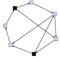
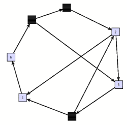
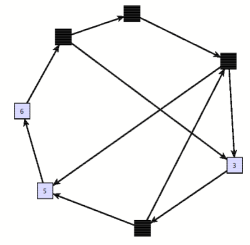
Figure 1: First two steps of UR starting from an initial network of 7 nodes, 2 of them being activated. Initially there is only one node among the non-activated nodes that satisfies the unanimity rule. It gets therefore activated at the first time step. At that time, there is a new node whose 2 incoming links come from activated nodes. It gets activated at the second time step. It is straightforward to show that this system gets fully activated at the fourth time step.

2 Unanimity model

The network is composed of $N$ nodes related through directed links. Each node exists in one of two states: activated or inactivated. The number of nodes with indegree $i$ (the indegree of a node is defined to be the number of links arriving to it) is denoted by $N_{i}$ and depends on the underlying network structure. Initially (at $t=0$) there are $A_{0}$ nodes which are activated, among which $A_{i,0}$ have an indegree $i$. In general, the number of nodes of type $i$, activated at time $t$, is $A_{i,t}$. It is also useful to introduce the quantities $n_{i}=\frac{N_{i}}{N}$ and $a_{i,t}=\frac{A_{i,t}}{N_{i}}$ which are the proportions of nodes of type $i$ in the network (indegree distribution) and the probability that such a node $i$ is activated, respectively. $a_{t}=\frac{A_{t}}{N}=\sum_{i}n_{i}a_{i,t}$ is the fraction of activated nodes in the whole network at time $t$. The unanimity rule is defined as follows (see Fig.1). At each time step, each node is considered. If all the links arriving to a specific unactivated node $i$ originate at nodes which are activated at $t-1$, $i$ gets activated at $t$. Otherwise, it remains unactivated. The process is applied iteratively until the system reaches a stationary state, characterized by an asymptotic value $a_{\infty}$. In the following, we are interested in the relation between $a_{\infty}$ and $a_{0}$, i.e. what is the final occupation of the network as a function of its initial occupation on a specific network. Let us mention the fact that each node may be produced by only one combination of (potentially many, depending on the indegree) nodes. This is a modification of the model of Hanel et al. [1], where more than one pairs of (two) nodes could produce new elements and will lead to a different equation for the activation evolution, as shown below. The dynamics studied here implies that nodes with a higher indegree will be activated with a probability smaller than those with a smaller indegree (because the former have more conditions to be fulfilled).

3 Master equation

Let us now derive an evolution equation for $A_{i,t}$ and $A_{t}$. To do so it is helpful to consider the first time step and than to iterate. There are initially $A_{0}$ activated nodes, $A_{i,0}=A_{0}N_{i}/N$ of them being of indegree $i$ on average (the activated nodes are randomly chosen in the beginning). The ensemble of $A_{i,0}$ nodes is called the initial set of indegree $i$. By construction, the probability that $i$ randomly chosen nodes are activated, is $a_{0}^{i}$ ($i$ is an exponent). Consequently, the average number of nodes with indegree $i$ and who respect the unanimity rule is $N_{i}a_{0}^{i}$ while the number of such nodes that are not yet occupied is

$$\Delta_{i,0}=(N_{i}-N_{i}a_{0})a_{0}^{i},$$ (1)

and, on average, the total number of occupied nodes with indegree $i$ evolves as:

$$A_{i,1}=A_{i,0}+\Delta_{i,0}.$$ (2)

Let us stress that we have implicitely assumed that there are no indegree correlations between neighboring nodes in order to derive Eq.1. At the next time step, the average number of nodes with indegree $i$, who respect the unanimity rule and who are outside the initial set is $(N_{i}-N_{i}a_{0})a_{1}^{i}$. Among those nodes, $\Delta_{0,i}$ have already been activated during the first time step, so that the average number of nodes who get activated at the second time step is:

$$\Delta_{i,1}=(N_{i}-N_{i}a_{0})(a_{1}^{i}-a_{0}^{i}).$$ (3)

Note that Eq.3 is valid because no node in $\Delta_{i,1}$ also belongs to $\Delta_{i,0}$. This is due to the fact that each node can only be activated by one combination of $i$ nodes in our model, so that no redundancy is possible between $\Delta_{i,1}$ and $\Delta_{i,0}$. By proceeding similarly, it is straightforward to show that the contributions $\Delta_{i,t}$ read

$$\Delta_{i,t}=(N_{i}-N_{i}a_{0})(a_{t}^{i}-a_{t-1}^{i}),$$ (4)

with $a_{-1}=0$ by convention. The number of activated nodes evolve as

$$A_{i,t+1}=A_{i,t}+\Delta_{i,t}.$$ (5)

By dividing by $N_{i}$, one gets a set of equations for the proportion of nodes $a_{i}\in[0,1]$:

$$a_{i,t+1}=a_{i,t}+(1-a_{0})(a_{t}^{i}-a_{t-1}^{i}),$$ (6)

where the coupling between the different proportions $a_{i,t}$ occurs through the average value $a_{t}=\sum_{i}n_{i}a_{i,t}$, as defined above. Finally, by multiplying by the indegree distribution $n_{i}$ and summing over all values of $i$, one gets a closed equation for the average proportion of activated nodes in the network that reads

$$a_{t+1}=a_{t}+(1-a_{0})\sum_{i}n_{i}(a_{t}^{i}-a_{t-1}^{i}).$$ (7)

Let us stress that Eq.7 is non-linear as soon as $N_{i}\neq 0$, $i>1$. Moreover, it is characterized by the non-trivial presence of the initial condition $a_{0}$ in the right hand non-linear term and is therefore highly non-local in time. Eq.7 explicitly shows how the indegree distribution $n_{i}$, affects the propagation of activated nodes in the system.

4 Theoretical results

In this section, we focus on simple choices of $n_{i}$ in order to apprehend analytically the behavior of Eq.7. The simplest case is $n_{1}=1$ for which Eq.7 reads

$$a_{t+1}=a_{t}+(1-a_{0})(a_{t}-a_{t-1}).$$ (8)

This equation is solved by recurrence:

$$a_{1} = a_{0}+(1-a_{0})a_{0}$$ (9)

$$a_{2} = a_{0}+(1-a_{0})a_{0}+(1-a_{0})[a_{0}+(1-a_{0})a_{0}-a_{0}]$$ (10)

$$= a_{0}+(1-a_{0})a_{0}+(1-a_{0})^{2}a_{0}$$ (11)

and in general

$$a_{t}=\sum_{u=0}^{t}(1-a_{0})^{u}a_{0}=1-(1-a_{0})^{t+1}.$$ (12)

This last expression is easily verified:

$$a_{t+1} = \sum_{u=0}^{t}(1-a_{0})^{u}a_{0}+(1-a_{0})(\sum_{u=0}^{t}(1-a_{0})^{u}a_{0}-\sum_{u=0}^{t-1}(1-a_{0})^{u}a_{0})$$ (13)

$$= \sum_{u=0}^{t}(1-a_{0})^{u}a_{0}+(1-a_{0})^{t+1}a_{0}=\sum_{u=0}^{t+1}(1-a_{0})^{u}a_{0}.$$ (14)

The above solution implies that any initial condition converges toward the asymptotic state $a_{\infty}=1$, i.e. whatever the initial condition, the system is fully activated in the long time limit. The relaxation to $a_{\infty}=1$ is exponentially fast $\sim e^{\ln(1-a_{0})t}$.

Figure 2: Numerical integration of Eq.15. In the left figure, we plot the time evolution of $a_{t}$, together with the theoretical prediction 17. In the right figure, we plot the relation $a_{\infty}(a_{0})$ that obviously shows a transition at $a_{0}=1/2$. Eq.17 is in perfect agreement with the numerical integration of Eq.15 (line). The agreement with the numerical simulations of the model itself is also excellent.

Let us now focus on the more challenging case $n_{2}=1$ where all the nodes have an indegree of 2 by construction. In that case, Eq. 7 reads

$$a_{t+1}=a_{t}+(1-a_{0})(a_{t}^{2}-a_{t-1}^{2}).$$ (15)

The non-linear term does not allow to find a simple recurrence expression as above. Though, a numerical integration of Eq.15 (by using Mathematica for instance) shows that the leading terms in the Taylor expansion of $a_{t}$ behave like

$$a_{t}=\sum_{i=1}^{t+1}a_{0}^{i}+{\cal O}(t+2)$$ (16)

thus suggesting that the asymptotic solution is

$$a_{\infty}=\frac{a_{0}}{1-a_{0}}.$$ (17)

This solution should satisfy the normalization constraint $a_{\infty}\leq 1$, so that it can hold only for initial conditions $a_{0}>1/2$. This argument suggest that a transition takes place at $a_{c}=1/2$, such that only a fraction of the whole system gets activated when $a_{0}<a_{c}$ while the whole system activates above this value (see Fig.2). We verify the approximate solution Eq.17 by looking for a solution of the form $a_{t}=\frac{a_{0}}{1-a_{0}}(1+\epsilon_{t})$. By insterting this expression into Eq.15, one gets the recurrence relations:

$$\epsilon_{t+1} = \epsilon_{t}+a_{0}(1+\epsilon_{t})^{2}-a_{0}(1+\epsilon_{t-1})^{2}$$ (18)

$$\epsilon_{t+1} = \epsilon_{t}+2a_{0}(\epsilon_{t}-\epsilon_{t-1}),$$ (19)

where the second line is obtained by keeping only first order corrections in $\epsilon$. In the continuous time limit, keeping terms until the second time derivative, one obtains

$$(1-2a_{0})\partial_{t}\epsilon_{t}+1/2(1+2a_{0})\partial_{t}^{2}\epsilon_{t}=0,$$ (20)

whose exponential solutions read $\epsilon_{t}=e^{-\lambda t}$ with

$$\lambda=\frac{1}{2}\frac{(1-2a_{0})}{(1+2a_{0})}.$$ (21)

This is a relaxation to the stationary state $a_{\infty}$ only when $a_{0}<1/2$, thereby confirming a qualitative change at $a_{c}=1/2$.

Figure 3: $a_{\infty}(a_{0})$ obtained for random networks with $L=2N$ (left figure). The measured indegree distribution is $n_{0}=0.14$, $n_{1}=0.27$, $n_{2}=0.27$… The No Zero and Zero versions (see text)are shown. In the right figure, $a_{\infty}(a_{0})$ for small-world networks $L=\lambda N$ short-cuts. When $\lambda=1$, the measured indegree distribution is $n_{0}=0.0$, $n_{1}=0.37$, $n_{2}=0.37$, etc. When $\lambda=2$, it is $n_{0}=0.0$, $n_{1}=0.14$, $n_{2}=0.27$… In both figures, the total number of nodes is $N=10000$ and the results are averaged over $100$ realizations of the process. The solid lines are the corresponding numerical solutions of Eq.22, evaluated with the empirical values $n_{i}$.

5 Some network topologies

Let us now focus on more reasonable topologies and compare the results obtained from Eq. 7 with numerical simulations of the UR. We focus on three types of networks, purely random networks [10], small-world like networks [11] and Barabasi-Albert networks [12] (growing networks with preferential attachment). The excellent agreement with Eq. 7 suggest that the formalism should apply to more general situations as well. The random network was obtained by randomly assigning $L$ directed links over $N$ nodes. The small-world network was obtained by starting from a directed ring configuration and than randomly assigning $L$ directed links (short-cuts) over the nodes, i.e. the total number of links in that case is $L+N$ (The network drawn in Fig.1 is such network with $N=7$ nodes and $L=3$ short-cuts). Let us note that the small-world network can be viewed as a food chain with a well-defined hierarchy between species together with some random short-cuts. In that case, UR can be interpreted as an extinction model (if all the species that one species eats go extinct, this species will also go extinct). The Barabasi-Albert network was built starting from one seed node and adding nodes one at a time until the system is composed of $N$ nodes. At each step, the node first connects to a randomly chosen node and, with probability $p$, it re-directs its link to the father of selected node. This method is well-known to be equivalent to preferential attachment and to lead to the formation of fat tail degree distributions $k^{\nu}$, with $\nu=1+1/p$, [13].

Figure 4: (left figure) distribution of indegrees for the scale-free network, $m_{i}=n_{i+1}$ (this shift being made to plot $n_{0}$ in log-log scale). The solid line is the theoretical asymptotical prediction $k^{-(1+1/p)}$, for $p=1/2$. The total number of nodes is $N=10000$, results are averaged over $100$ realizations of the process. (right figure) $a_{\infty}(a_{0})$ for the same network. In the No Zero version, one observes that the all the nodes are finally activated whatever the initial condition. The solid lines correspond to numerical values of Eq.22 for the empirical values $n_{i}$.

Once the underlying network is built, we randomly assign $a_{0}N$ active nodes to the network and apply the unanimity rule. The evolution stops once a stationary state is reached. The asymptotic value $a_{\infty}$ is averaged over several realizations of the process (on several realizations of the underlying network). In the small-world network, each node receives at least one incoming link. This is not the case for the random- or the BA networks, for which one has to discuss the ambiguous dynamics of nodes with zero incoming links. Two choices are possible. Either these nodes can not be activated in the course of time, because they are not reached by any other node (No Zero version), or all of them are get activated at the first time step, thereby assuming that their activation does not require any first knowledge (Zero version). The choise is a question of interpretation. The two versions are associated to different evolution equations:

$$a_{t+1} = a_{t}+(1-a_{0})\sum_{i=1}^{\infty}n_{i}(a_{t}^{i}-a_{t-1}^{i})~{}~{}{\rm No}~{}{\rm Zero}~{}{\rm version}$$ (22)

$$a_{t+1} = a_{t}+(1-a_{0})\sum_{i=0}^{\infty}n_{i}(a_{t}^{i}-a_{t-1}^{i})~{}~{}{\rm Zero}~{}{\rm version},$$ (23)

and leads to quite different behaviors (Figs.3 and 4). In the case of small-world networks, the above equations are obviously equivalent. To compare the simulation results with Eq.22, we also measure the indegree distributions of the networks $n_{i}$ generated during the simulations and integrate Eq.22 with these empirical values. The agreement is excellent, except close to the transition points where finite size effects are expected. It is worth noting that the importance of nodes with zero incoming links is much higher in (growing) Barabasi-Albert like networks (Fig.4), so that the difference between the two versions is quite pronounced, as expected. Let us also mention that Eq.14 has been successfully verified for a random network where the indegree of each node is exactly 2 ($n_{2}=1$), as shown in Fig.2.

6 Discussion

In this Letter, we have introduced a simple model for innovation whose dynamics is based on Unanimity Rule. It is shown that the discovery of new items on the underlying network opens perspectives for the discovery of new items. This feedback effect may lead to complex spreading properties, embodied by the existence of a critical size for the initial activation, that is necessary for the complete activation of the network in the long time limit. The problem has been analyzed empirically on a large variety of network structures and has been successfully described by recurrence relations for the average activation. Let us stress that these recurrence relations have a quite atypical form, due to their explicit dependence on the initial conditions. Moreover, their non-linearity makes them a hard problem to solve in general. Finally, let us insist on the fact that Unanmity Rule is a general mechanism that should apply to numerous situations related to innovation, opinion dynamics or even species/population dynamics. To be consistent with our own work, we also hope that this paper will trigger the reader’s curiosity and, possibly, open new perspectives or research directions…

Acknowledgements This collaboration was made possible by a COST-P10 short term mission. R.L. has been supported by European Commission Project CREEN FP6-2003-NEST-Path-012864. S.T. is grateful to Austrian Science Foundation projects P17621 and P19132.

References

- [1] R. Hanel, S. A. Kauffman and S.Thurner, Phys. Rev. E 72, 036117 (2005).
- [2] J. D. Farmer, S.A. Kauffman, N. H. Packard, Physica D 22, 50 (1986).
- [3] S. A. Kauffman, The Origins of Order (Oxford University Press, London, 1993).
- [4] P. F. Stadler, W. Fontana, J. H. Miller, Physica D 63, 378 (1993).
- [5] S. Galam, Physica 274, 132 (1999).
- [6] K. Sznajd-Weron and J. Sznajd, Int. J. Mod. Phys. C 11, 1157 (2000).
- [7] P. L. Krapivsky and S. Redner, Phys. Rev. Lett. 90, 238701 (2003).
- [8] C. Castellano, D. Vilone, and A. Vespignani, Europhys. Lett. 63, 153 (2003).
- [9] K. Suchecki and J. A. Hołyst, Physica A 362 338 (2006).
- [10] P. Erdős and A. Rényi, Publ. Math. Inst. Hung. Acad. Sci. 5, 17–61 (1960).
- [11] D. J. Watts, and S. H. Strogatz, Nature 393, 440 (1998).
- [12] A.-L. Barabási and R. Albert, Science 286, 509 (1999).
- [13] P. L. Krapivsky and S. Redner, Phys. Rev. E 63, 066123 (2001).