Directed or Undirected? A New Index to Check
for Directionality of Relations in Socio-Economic Networks

Abstract

This paper proposes a simple procedure to decide whether the empirically-observed adjacency or weights matrix, which characterizes the graph underlying a socio-economic network, is sufficiently symmetric (respectively, asymmetric) to justify an undirected (respectively, directed) network analysis. We introduce a new index that satisfies two main properties. First, it can be applied to both binary or weighted graphs. Second, once suitably standardized, it distributes as a standard normal over all possible adjacency/weights matrices. To test the index in practice, we present an application that employs a set of well-known empirically-observed social and economic networks.

I Introduction

In the last years, the literature on networks has been characterized by exponential growth. Empirical and theoretical contributions in very diverse fields such as physics, sociology, economics, etc. have increasingly highlighted the pervasiveness of networked structures. Examples range from WWW, the Internet, airline connections, scientific collaborations and citations, trade and labor market contacts, friendship and other social relationships, business relations and R&S partnerships, all the way through cellular, ecological and neural networks Albert and Barabási (2002); Newman (2003); Wasserman and Faust (1994); Carrington et al. (2005).

The empirical research has thoroughly studied the (often complex) topological properties of such networks, whereas a large number of theoretical models has been proposed in order to investigate how networks evolve through time Dorogovtsev and Mendes (2003). Structural properties of networks have been shown to heavily impact on the dynamics of the socio-economic systems that they embed Watts (1999). As a result, their understanding has become crucial also as far as policy implications are concerned Granovetter (1974).

The simplest mathematical description of a network is in terms of a graph, that is a list of nodes $\{1,2,...,N\}$ and a set of arrows (links), possibly connecting any two nodes Harary (1969); Bollobás (1985). Alternatively, one can characterize a network through a $N\times N$ real-valued matrix $W=\{w_{ij}\}$, where any out-of-diagonal entry $w_{ij}$ is non-zero if and only if an arrow from node $i$ to $j$ exists in the network. Entries on the main diagonal are typically assumed to be all different from zero (if self-interactions are allowed) or all equal to zero (if they are not). Networks are distinguished in binary (dichotomous) or weighted. In binary networks all links carry the same intensity. This means that in binary networks a link is either present or not, i.e. $w_{ij}\in\{0,1\}$. In this case, $W$ is called an “adjacency” matrix. Weighted networks allow one instead to associate a weight (i.e. a positive real number) to each link, typically proportional to its interaction strength or the flux intensity it carries Barrat et al. (2004, 2005); Barthélemy et al. (2005); DeMontis et al. (2005). Any non-zero entry $w_{ij}$ thus measures the weight of the link originating from $i$ and ending up in $j$, and the resulting matrix $W$ is called the “weights” matrix .

Both binary and weighted networks can be undirected or directed. Formally, a network is undirected if all links are bilateral, i.e. $w_{ij}w_{ji}>0$ for all $i\neq j$. This means that in undirected networks all pairs of connected nodes mutually affect each other. One can thus replace arrows with non-directed edges (or arcs) connecting any two nodes and forget about the implicit directions. This greatly simplifies the analysis, as the tools for studying undirected networks are much better developed and understood. Directed networks are instead not symmetric, as there exists at least a pair of connected nodes wherein one directed link is not reciprocated, i.e. $\exists(i,j),i\neq j:w_{ij}>0$, but $w_{ji}=0$. Studying the topological properties of directed networks, especially in the weighted case, can become more difficult, as one has to distinguish inward from outward links in computing synthetic indices such as node and average nearest-neighbor degree and strength, clustering coefficient, etc.. Therefore, it is not surprising that the properties of such indices are much less explored in the literature.

From a theoretic perspective, it is easy to distinguish undirected from directed networks: the network is undirected if and only if the matrix $W$ is symmetric. When it comes to the empirics, however, researchers often face the following problem. If the empirical network concerns an intrinsically mutual social or economic relationship (e.g. friendship, marriage, business partnerships, etc.) then $W$, as estimated by the data collected, is straightforwardly symmetric and only tools designed for undirected network analysis are to be employed. More generally, however, one deals with notionally non-mutual relationships, possibly entailing directed networks. In that case, data usually allow to build a matrix $W$ that, especially in the weighted case, is hardly found to be symmetric. Strictly speaking, one should treat all such networks as directed. This often implies a more complicated and convoluted analysis and, frequently, less clear-cut results. The alternative, typically employed by practitioners in the field, is to compute the ratio of the number of directed (bilateral) links actually present in the networks to the maximum number of possible directed links (i.e. $N(N-1)$). If this ratio is “reasonably” large, then one can symmetrize the network (i.e. making it undirected, see Wasserman and Faust (1994); De Nooy et al. (2005)) and apply the relevant undirected network toolbox.

However, as shown in Ref. Garlaschelli and Loffredo (2004a), this procedure has several drawbacks. In particular, it is heavily dependent on the density of the network under analysis (i.e., the ratio between the total number of existing links to $N(N-1)$).

Moreover, and most important here, if the network is weighted, the ratio of bilateral links does not take into account the effect of link weights. Indeed, a bilateral link exists between $i$ and $j$ if and only if $w_{ij}w_{ji}>0$, i.e. irrespective of the actual size of the two weights. Of course, as far as symmetry of $W$ is concerned, the sub-case where $w_{ij}>>0,w_{ji}\simeq 0$ will be very different from the sub-case where $w_{ij}\simeq w_{ji}>0$.

In this paper, we present a simple procedure that tries to overcome this problem. More specifically, we develop a simple index that can help in deciding when the empirically-observed $W$ is sufficiently symmetric to justify an undirected network analysis. Our index has two main properties. First, it can be applied with minor modifications to both binary and weighted networks. Second, the standardized version of the index distributes as a standard normal (over all possible matrices $W$). Therefore, after having set a threshold $x$, one might conclude that the network is to be treated as if it is undirected if the index computed on $W$ is lower than $x$.

Of course, the procedure that we propose in the paper is by no means a statistical test for the null hypothesis that $W$ involves some kind of symmetry. Indeed, one has almost always to rely on a single observation for $W$ (more on that in Section V). Nevertheless, we believe that the index studied here could possibly provide a simple way to ground the “directed vs. undirected” decision on more solid bases.

The paper is organized as follows. In Section II we define the index and we derive its basic properties. Section III discusses its statistical properties, while in Section IV we apply the procedure to the empirical networks extensively studied in Wasserman and Faust (1994). Finally, Section V concludes.

II Definition and Basic Properties

Consider a directed, weighted, graph $\widetilde{G}=(N,\widetilde{A})$, where $N$ is the number of nodes and $A=\{\widetilde{a}_{ij}\}$ is the $N\times N$ (real-valued) matrix of link “weights” Barrat et al. (2004); Barthélemy et al. (2005); Barrat et al. (2005); DeMontis et al. (2005). Without loss of generality, we can assume $\widetilde{a}_{ij}\in[0,1],\forall i\neq j$ and $\widetilde{a}_{ii}=\widetilde{a}\in\{0,1\},i,j=1,\dots\,N$ . In line with social network analysis, we interpret the generic out-of-diagonal entry $\widetilde{a}_{ij},i\neq j$, as the weight associated to the directed link originating from node $i$ and ending up in node $j$ (i.e., the strength of the directed link $i\rightarrow j$ in the graph). A directed edge from $i$ to $j$ is present if and only if $\widetilde{a}_{ij}>0$.

The idea underlying the construction of the index is very simple. If the graph $\widetilde{G}$ is undirected, then $\widetilde{A}=\widetilde{A}^{T}$, where $\widetilde{A}^{T}$ is the transpose of $\widetilde{A}$. Denoting by $\|\cdot\|$ any norm defined on a square-matrix, the extent to which directionality of links counts in the graph $\widetilde{G}$ can therefore be measured by some increasing function of $\|\widetilde{A}-\widetilde{A}^{T}\|$, suitably rescaled by some increasing function of $\|\widetilde{A}\|$ (and possibly of $\|\widetilde{A}^{T}\|$).

To build the index we first define, again without loss of generality:

$$A=\{a_{ij}\}=\widetilde{A}-(1-\widetilde{a})I_{N},$$ (1)

where $I_{N}$ is the $N\times N$ identity matrix. Accordingly, we define the graph $G=(N,A)$. Notice that $a_{ij}=\widetilde{a}_{ij}$ for all $i\neq j$, while now $a_{ii}=1$ for all $i$.

Consider then the square of the Frobenius (or Hilbert-Schmidt) norm:

$$\|A\|_{F}^{2}=\sum_{i}\sum_{j}{a_{ij}^{2}}=N+\sum_{i}\sum_{j\neq i}{a_{ij}^{2}},$$ (2)

where all sums (also in what follows) span from 1 to $N$. Notice that $\|A\|_{F}^{2}$ is invariant with respect to the transpose operator, i.e. $\|A\|_{F}=\|A^{T}\|_{F}$.

We thus propose the following index:

$$\widetilde{S}(A)=\frac{\|A-A^{T}\|_{F}^{2}}{\|A\|_{F}^{2}+\|A^{T}\|_{F}^{2}}=\frac{\|A-A^{T}\|_{F}^{2}}{2\|A\|_{F}^{2}}=\frac{1}{2}\left[\frac{\|A-A^{T}\|_{F}}{\|A\|_{F}}\right]^{2}.$$ (3)

By exploiting the symmetry of $(a_{ij}-a_{ji})^{2}$, one easily gets:

$$\widetilde{S}(A)=\frac{\sum_{i}\sum_{j}{(a_{ij}-a_{ji})^{2}}}{2\sum_{i}\sum_{j}{a_{ij}^{2}}}=\frac{\sum_{i}\sum_{j>i}{(a_{ij}-a_{ji})^{2}}}{N+\sum_{i}\sum_{j\neq i}{a_{ij}^{2}}}.$$ (4)

Alternatively, by expanding the squared term at the numerator, we obtain:

$$\widetilde{S}(A)=1-\frac{\sum_{i}\sum_{j}{a_{ij}a_{ji}}}{\sum_{i}\sum_{j}{a_{ij}^{2}}}=1-\frac{N+\sum_{i}\sum_{j\neq i}{a_{ij}a_{ji}}}{N+\sum_{i}\sum_{j\neq i}{a_{ij}^{2}}}=$$ (5)

$$=1-\frac{N+2\sum_{i}\sum_{j>i}{a_{ij}a_{ji}}}{N+\sum_{i}\sum_{j\neq i}{a_{ij}^{2}}}=\frac{\sum_{i}\sum_{j\neq i}{a_{ij}^{2}}-2\sum_{i}\sum_{j>i}{a_{ij}a_{ji}}}{N+\sum_{i}\sum_{j\neq i}{a_{ij}^{2}}}.$$ (6)

The index $\widetilde{S}(A)$ has a few interesting properties, which we summarize in the following:

Lemma 1 (General properties of $\widetilde{S}$)

For all real-valued $N\times N$ matrices $A=\{a_{ij}\}$ s.t. $a_{ij}\in[0,1],i\neq j$ and $a_{ii}=1,i=1,...,N$, then:

1. $\widetilde{S}(A)\geq 0$.

2. $\widetilde{S}(A)=0\Leftrightarrow A=A^{T}$, i.e. if and only if the graph is undirected.

3. $\widetilde{S}(A)\leq\frac{N-1}{N+1}$

Proof. See Appendix A.   

Furthermore, when $G$ is binary (i.e., $a_{ij}\in\{0,1\}$ for all $i,j$), the index in eq. 3 turns out to be closely connected to the density of the graph (i.e., the ratio between the total number of directed links to the maximum possible number of directed links) and the ratio of the number of bilateral directed links in $G$ (i.e. links from $i$ to $j$ s.t. $a_{ij}=a_{ji}=1$) to the maximum possible number of directed links. More precisely:

Lemma 2 (Properties of $\widetilde{S}$ in the case of binary graphs)

When $G$ is binary, i.e. $a_{ij}\in\{0,1\}$, all $i,j$, then:

$$\widetilde{S}(A)=\frac{d(A)-b(A)}{(N-1)^{-1}+d(A)}.$$ (7)

where $d(A)$ is the density of $G$ and $b(A)$ is the ratio between the number of bilateral directed links to the maximum number of directed links.

Proof. See Appendix B.   

Notice that, in the case of undirected graphs, $b(A)=d(A)$ and $\widetilde{S}(A)=0$. On the contrary, when there are no bilateral links, $b(A)=0$. Hence, $\widetilde{S}(A)=[d(A)/(N-1)+1]^{-1}$, which is maximized when $d(A)=\frac{1}{2}$, i.e. $\widetilde{S}(A)=\frac{N-1}{N+1}$, as shown in Lemma 1. Obviously, the larger $b(A)$, the more the graph $G$ is undirected. As mentioned in Section I, $b(A)$ can be employed to check for the extent to which directionality counts in $G$. However, such index is not very useful in weighted graphs, as it does not take into account the size effect (i.e. the size of weights as measured by $a_{ij}\in[0,1]$).

In the case of binary graphs, the index in (3) almost coincides with the one proposed in Garlaschelli and Loffredo (2004a). They suggest to employ the correlation coefficient between $(a_{ij},a_{ji})$ entries in the adjacency matrix (excluding self loops). It can be shown that this alternative index – unlike the one in (3) – increases with the number of reciprocated links, only if both the total number of links that are in place and the density of the network remain constant. See also Garlaschelli and Loffredo (2004b); Garlaschelli and Loffredo (2005) for applications.

Since $\widetilde{S}(A)\in[0,\frac{N-1}{N+1}]$, in what follows we shall employ its rescaled version:

$$S(A)=\frac{N+1}{N-1}\widetilde{S}(A),$$ (8)

which ranges in the unit interval and thus has a more straightforward interpretation.

III Statistical Properties

In this section we study the distribution of the index $S$ as defined in eqs. 3 and 8. Indeed, despite the range of $S$ does not depend on $N$, we expect its distribution to be affected by: (i) the size of the matrix ($N$); (ii) whether the underlying graph $G$ is binary ($a_{ij}\in\{0,1\}$) or weighted ($a_{ij}\in[0,1]$).

To do so, for each $N\in\{5,10,50,100,200,500,700,1000\}$ we generate $M=100,000$ random matrices $A$ obeying the restriction that $a_{ii}=1$, all $i$. In the binary case, out-of-diagonal entries $\{a_{ij},i\neq j\}$ are drawn from i.i.d. Bernoulli random variables with $prob\{a_{ij}=0\}=prob\{a_{ij}=1\}=0.5$. In the weighted case, entries $a_{ij}$ are i.i.d. random variables uniformly-distributed over $[0,1]$. We then estimate the distributions of $S$ in both the binary and the weighted cases, and we study their behavior as the size of the graph increases. Let us denote by $m_{B}(N)$ (respectively, $m_{W}(N)$) the sample mean of the index $S$ in the binary (respectively, weighted) case, and by $s_{B}(N)$ (respectively, $s_{W}(N)$) the sample standard deviation of the index $S$ in the binary (respectively, weighted) case. Simulation results are summarized in the following points.

1. In both the binary and the weighted case, the index $S$ approximately distributes as a Beta random variable for all $N$. As $N$ increases, $m_{B}(N)$ decreases towards 0.50 whereas $m_{W}(N)$ increases towards 0.25. Both standard deviations decrease towards 0. More precisely, the following approximate relations hold (see Figures 2 and 2):

   $$m_{B}(N)\simeq 0.50+exp\{-1.786369-1.680938lnN\}$$ (9)

   $$m_{W}(N)\simeq 0.25-exp\{-1.767551-0.937586lnN\}$$ (10)

   $$s_{B}(N)\simeq exp\{-0.135458-1.001695lnN\}$$ (11)

   $$s_{W}(N)\simeq exp\{-0.913297-0.982570lnN\}$$ (12)

   

   Figure 1: Binary Graphs. Sample mean and standard deviation of $S$ vs. $N$, together with OLS fits. Log-scale on both axes. OLS fits: $ln[m_{B}(N)-0.50]\simeq-1.786369-1.680938lnN$ ($R^{2}=0.998934$) and $ln[s_{B}(N)]\simeq-0.135458-1.001695lnN$ ($R^{2}=0.999995$).

   

   Figure 2: Weighted Graphs. Sample mean and standard deviation of $S$ vs. $N$, together with OLS fits. Log-scale on both axes. OLS fits: $ln[0.25-m_{W}(N)]\simeq-1.767551-0.937586lnN$ ($R^{2}=0.998966$) and $ln[s_{W}(N)]\simeq-0.913297-0.982570lnN$ ($R^{2}=0.999932$).

2. Given the approximate relations in eqs. 9-12, let us standardize the index $S$ as follows:

   $$S_{B}(A)=\frac{S(A)-m_{B}(N)}{s_{B}(N)},$$ (13)

   $$S_{W}(A)=\frac{S(A)-m_{W}(N)}{s_{W}(N)}.$$ (14)

   Simulations indicate that the standardized versions of the index, i.e. $S_{B}$ and $S_{W}$, are both well approximated by a $N(0,1)$, even for small $N$s ($N\geq 10$). Indeed, as Figures 4 and 4 show, the mean of the distributions of $S_{B}$ and $S_{W}$ vs. $N$ converges towards zero, while the standard deviation approaches one (we actually plot standard deviation minus one to have a plot in the same scale). Also the third (skewness) and the fourth moment (excess kurtosis) stay close to zero. We also plot the estimated distribution of $S_{B}$ and $S_{W}$ vs. $N$, see Figures 6 and 6. It can be seen that all estimated densities collapse towards a $N(0,1)$. Notice that the y-axis is in log scale: this allows one to appreciate how close to a $N(0,1)$ are the distributions for all $N$ on the tails.

   

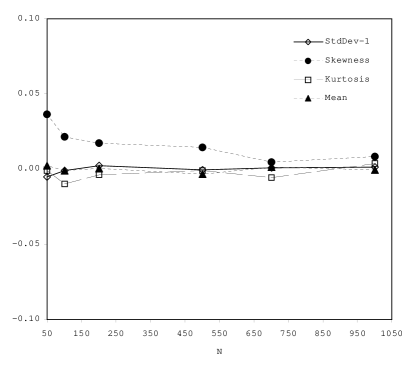
   Figure 3: Binary Graphs. Moments of $S_{B}$ vs. $N$.

   

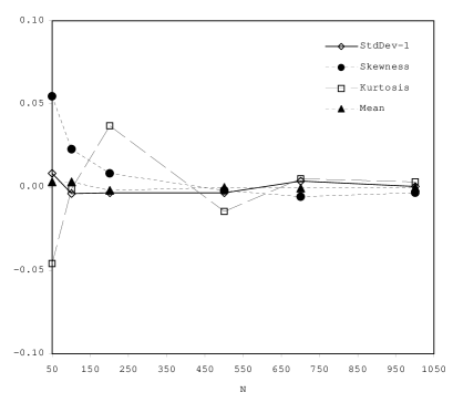
   Figure 4: Weighted Graphs. Moments of $S_{W}$ vs. $N$.

   

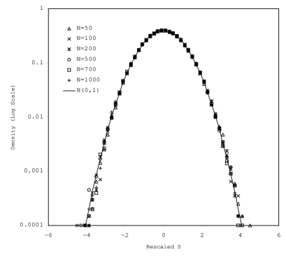
   Figure 5: Binary Graphs. Estimated distribution of $S_{B}$ vs. $N$. The $N(0,1)$ fit is also shown as a solid line.

   

   Figure 6: Weighted Graphs. Estimated distribution of $S_{W}$ vs. $N$. The $N(0,1)$ fit is also shown as a solid line.

   Notice finally that as $N$ increases, the distribution maintains a constant second moment but the range increases linearly with $N$, see 8 and 8. The lower bound (LB) and the upper bound (UB) indeed read approximately:

   

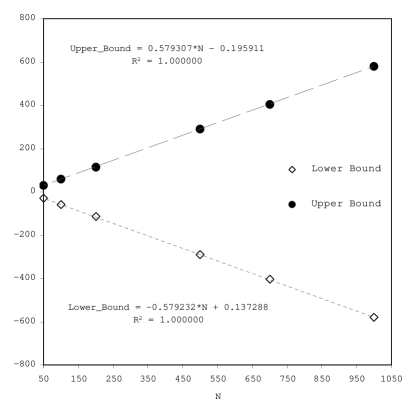
   Figure 7: Binary Graphs. Lower and upper bounds of the re-scaled index $S_{B}$ vs. $N$, together with the OLS fit.

   

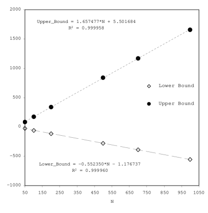
   Figure 8: Weighted Graphs. Lower and upper bounds of the re-scaled index $S_{W}$ vs. $N$, together with the OLS fit.

   $$LB_{\ast}(N)=\simeq-\frac{m_{\ast}(N)}{s_{\ast}(N)},UB_{\ast}(N)=\simeq\frac{1-m_{\ast}(N)}{s_{\ast}(N)}$$ (15)

   where $\{\ast\}=\{B,W\}$ stands for binary (B) and weighted (W). Since the standardized index is well approximated by a $N(0,1)$ for all $N$, this means that extreme values become more and more unlikely. This is intuitive, because as $N$ grows the number of matrices with highest/lowest values of the index are very rare.

IV Examples

The index developed above can be easily employed to assess the extent to which link directionality matters in real-world networks. Let us suppose to have estimated a $N\times N$ matrix $X=\{x_{ij}\}$ describing a binary (B) or a weighted (W) graph. We then compute the index:

$$S_{\ast}(X)=\frac{\frac{N+1}{N-1}\widetilde{S}(X)-m_{\ast}(N)}{s_{\ast}(N)}=$$ (16)

$$=\frac{1}{s_{\ast}(N)}\left[\frac{N+1}{N-1}\frac{\sum_{i}\sum_{j>i}{(x_{ij}-x_{ji})^{2}}}{N+\sum_{i}\sum_{j\neq i}{x_{ij}^{2}}}-m_{\ast}(N)\right].$$ (17)

where $\{\ast\}=\{B,W\}$ and $(m_{\ast}(N),s_{\ast}(N))$ are as in eqs. 9-12. Since we know that $S_{\ast}(X)$ is approximately $N(0,1)$, we can fix a lower threshold in order to decide whether the network is sufficiently (un)directed. For instance, we could set the lower threshold equal to 0 (i.e. equal to the mean), and decide that if $S_{\ast}(X)>0$ (above the mean) we shall treat the network as directed (and undirected otherwise). More generally, one might set a threshold equal to $x\in R$ and conclude that the graph is undirected if $S_{\ast}<x$. On the contrary, one should expect the directional nature of the graph to be sufficiently strong, so that a digraph analysis is called for.

To test the index against real-world cases, we have taken the thirteen social and economic networks analyzed in Wasserman and Faust (1994), see Table 1 . All networks are binary and directed, apart from Freeman’s ones (which are weighted and directed) and Padgett’s ones (which are binary and undirected). Table 1 reports both the index $S$ and its standardized versions $S_{\ast},\{\ast\}=\{B,W\}$, for all cited examples.

Table 1: The index $S$ and its standardized version $S_{\{\ast\}},\{\ast\}=\{B(inary),W(eigthed)\}$ for social networks studied in Wasserman and Faust (1994), cf. Chapter 2.5.

	Social Network	$N$	$S$	$S_{\ast}$
1	Advice relations btw Krackhardt’s hi-tech managers	21	0.521327	0.491228
2	Friendship relations btw Krackhardt’s hi-tech managers	21	0.500813	0.004610
3	“Reports-to” relations btw Krackhardt’s hi-tech managers	21	0.536585	0.860033
4	Business relationships btw Padgett’s Florentine families	16	0.000000	-9.232823
5	Marital relationships btw Padgett’s Florentine families	16	0.000000	-9.232823
6	Acquaintanceship among Freeman’s EIES researchers (Time 1)	32	0.109849	-10.025880
7	Acquaintanceship among Freeman’s EIES researchers (Time 2)	32	0.094968	-11.143250
8	Messages sent among Freeman’s EIES researchers	32	0.014548	-17.181580
9	Country Trade Flows: Basic Manufactured Goods	24	0.260349	-6.643695
10	Country Trade Flows: Food and Live Animals	24	0.311966	-5.217508
11	Country Trade Flows: Crude Materials (excl. Food)	24	0.272560	-6.306300
12	Country Trade Flows: Minerals, Fuels, Petroleum	24	0.403336	-2.692973
13	Country Trade Flows: Exchange of Diplomats	24	0.080208	-11.620970

Suppose to fix the lower threshold equal to zero. Padgett’s networks, being undirected, display a very low value (in fact, the non standardized index is equal to zero as expected). The table also suggests to treat all the binary trade networks as undirected. The same advice applies for Freeman’s networks, which are instead weighted. The only networks which have an almost clear directed nature (according to our threshold) are Krackhardt’s ones. In that case our index indicates that a directed graph analysis would be more appropriate.

V Concluding Remarks

In this paper we have proposed a new procedure that might help to decide whether an empirically-observed adjacency or weights $N\times N$ matrix $W$, describing the graph underlying a social or economic network, is sufficiently symmetric to justify an undirected network analysis. The index that we have developed has two main properties. First, it can be applied to both binary or weighted graphs. Second, once suitably standardized, it distributes as a standard normal over all possible adjacency/weights matrices. Therefore, given a threshold decided by the researcher, any empirically observed adjacency/weights matrix displaying a value of the index lower (respectively, higher) than the threshold is to be treated as if it characterizes an undirected (respectively, directed) network.

It must be noticed that setting the threshold always relies on a personal choice, as also happens in statistical hypothesis tests with the choice of the significance level $\alpha$. Despite this unavoidable degree of freedom, the procedure proposed above still allows for a sufficient comparability among results coming from different studies (i.e. where researchers set different threshold) if both the value of the index $S$ and the size of the network are documented in the analysis. In that case, one can easily compute the probability of finding a matrix with a lower/higher degree of symmetry, simply by using the definition of bounds (see eq. 15) and probability tables for the standard normal.

A final remark is in order. As mentioned, our procedure does not configure itself as a statistical test. Since the researcher often relies on a single observation of the network under study (or a sequence of serially-correlated network snapshots through time), statistical hypothesis testing will be only very rarely feasible. Nevertheless, in the case where a sample of $M$ i.i.d. observations of $W$ is available, one might consider to use the the sample average of the index (multiplied by $\sqrt{M}$) and employ the cental limit theorem to test the hypothesis that the observations come from a undirected (random) graph.

Appendix A Proof of Lemma 1

Points (1) and (2) simply follow from the definition in eq. 3. As to (3), let us suppose that there exists a matrix $A$ satisfying the above restrictions and such that $\widetilde{S}(A)>\frac{N-1}{N+1}$. Then, using eq. 6:

$$\frac{N+2\sum_{i}\sum_{j>i}{a_{ij}a_{ji}}}{N+\sum_{i}\sum_{j\neq i}{a_{ij}^{2}}}<\frac{2}{N+1}.$$ (18)

The best case for such an inequality to be satisfied is when the the left hand side is minimized. This is achieved when there are $N(N-1)/2$ entries equal to one and $N(N-1)/2$ entries equal to zero in such a way that $a_{ij}\neq a_{ji}$ for all $i\neq j$ (e.g., when the upper diagonal matrix is made of all ones and the lower diagonal matrix is made of all zeroes). In that case the left hand side is exactly equal to $\frac{2}{N+1}$, leading to the absurd conclusion that $\frac{2}{N+1}<\frac{2}{N+1}$.

Appendix B Proof of Lemma 2

It follows from the definition of $d(A)$ that:

$$d(A)=\frac{\sum_{i}\sum_{j\neq i}{a_{ij}}}{N(N-1)}=\frac{\sum_{i}\sum_{j\neq i}{a_{ij}^{2}}}{N(N-1)},$$ (19)

Moreover, it is easy to see that:

$$b(A)=\frac{\sum_{i}\sum_{j\neq i}{a_{ij}a_{ji}}}{N(N-1)}=\frac{2\sum_{i}\sum_{j>i}{a_{ij}a_{ji}}}{N(N-1)}.$$ (20)

To prove the Lemma, it suffices to note that:

$$\widetilde{S}(A)=1-\frac{N+2\sum_{i}\sum_{j>i}{a_{ij}a_{ji}}}{N+\sum_{i}\sum_{j\neq i}{a_{ij}^{2}}}=$$ (21)

$$=1-\frac{1+(N-1)b(A)}{1+(N-1)d(A)}=\frac{d(A)-b(A)}{(N-1)^{-1}+d(A)}.$$ (22)