Low complexity method for large-scale self-consistent ab initio electronic-structure calculations without localization

Abstract

A novel low complexity method to perform self-consistent electronic-structure calculations using the Kohn-Sham formalism of density functional theory is presented. Localization constraints are neither imposed nor required thereby allowing direct comparison with conventional cubically scaling algorithms. The method has, to date, the lowest complexity of any algorithm for an exact calculation. A simple one-dimensional model system is used to thoroughly test the numerical stability of the algorithm and results for a real physical system are also given.

Low complexity electronic-structure methods , using the Kohn-Sham density functional approach Hohenberg and Kohn (1964); Kohn and Sham (1965), where the operation count scales with respect to system size (‘$N$-scaling’) as $N^{\alpha}$ where $\alpha\leq 2$ have been around for a few decades. A comprehensive review of low complexity methods is given in reference Goedecker (1999). Contrary to what is often reported the theoretical upper bound for the $N$-scaling of an exact self-consistent algorithm has been set at $\mathcal{O}(N^{2})$ ever since Fermi operator expansion (FOE) methods were developed Goedecker and Colombo (1994). This letter shows how the theoretical upper bound for the scaling of such calculations can be lowered to $\mathcal{O}(\alpha(d,N){N^{\frac{2d-1}{d}}})$ where $d$ is the dimensionality of repetition of a full three-dimensional system and $\alpha(1,N)=\log_{2}(N)$, $\alpha(2,N)\leq 2$ and $\alpha(3,N)\leq 4/3$. For large scale calculations low complexity algorithms are without doubt the future of electronic-structure implementations. However, low complexity ab initio algorithms are not in common usage at the moment, primarily due to two main reasons. Firstly, much of the work currently being carried out deals with systems that are too small to be amenable to low complexity approaches if high accuracy is desired. Secondly, low complexity algorithms are not yet fully functional and fully stable for general systems - so a sufficient level of confidence in using these codes has not been established. While the first reason is rapidly being diminished due to the ever reducing cost of a floating point operation, the second may prove to be far more stubborn.

Most low complexity algorithms fall broadly into two categories; either they attempt to calculate localized orbitals or they seek to evaluate the density matrix (DM) directly. For a general system only the latter is known to provide a low complexity solution. In the case of a metal, for example, delocalized states at the Fermi level prevent the occupied subspace being represented in terms of orthogonal localized orbitals.

Problems associated with low complexity approaches commonly stem from the imposition of a priori localization constraints. The effect of this restriction varies depending on the algorithm and physical system. In orbital minimization algorithms even the initial guess can alter the obtained solution. In some cases localization will always cast a degree of doubt over the final answers (except in the simplest wide-gap systems), and in others prohibits obtaining the relevant physics/chemistry all together. Fermi operator expansion (FOE) algorithms (either using a polynomial Goedecker and Colombo (1994); Goedecker and Teter (1995) or rational Goedecker (1995) approximation) for systems with a DM localized in real-space provide arguably the most natural and foolproof way of obtaining results in $\mathcal{O}(N)$. In these methods the locality does not necessarily have to be imposed a priori, rather the system can be allowed to inform us of the locality in a systematic way. Methods that impose unsystematic localization are invariably open to more doubt. While a great deal of progress has been made in understanding the inherent locality present in many systems, low temperature metallic systems and charged insulating systems with long-ranged DM correlations are still a significant challenge. The method presented in this letter is primarily aimed at such systems. However, it has also been noted that the onset of sparsity of the DM, even for wide-gap systems, is ‘discouragingly slow’ Maslen et al. (1998) especially if high accuracy is required. The main advantage of the method in this work is that it relies purely on the locality of the basis functions allowing the use of non-orthogonal localized basis sets, such as Gaussians, with rather less localized orthogonal and dual complements. Also, the full DM need not be explicitly calculated.

The energy renormalization group (ERG) approach Baer and Head-Gordon (1998a, b); Kenoufi and Polonyi (2004) is a beautiful and elegant concept that has also been suggested to cope with such difficult problems. In an ideal implementation it may be possible for its scaling to better the method given here for $d>1$ and equal it for $d=1$. However, it remains unclear whether an ERG algorithm can also provide the density in an efficient manner and to some extent the ERG method employs cutoffs. Therefore, the ERG method will not be included in the definition of FOE methods in the following.

To date, standard FOE methods have been considered to scale quadratically for systems where the DM decay length is of the order of the system size. This can be the case for very large systems especially for metals at low temperature or if high accuracy is required. The method presented here imposes no localization constraints and scales as $\mathcal{O}(\alpha(d,N){N^{\frac{2d-1}{d}}})$ where $\alpha(d,N)$ is a weak logarithmic factor for $d=1$ and tends to a constant in higher dimensions. Not only does this represent a new theoretical upper bound for the $N$-scaling of an exact algorithm (upto the basis set limit) it is also expected to make a significant and immediate impact on systems of low dimensionality. Furthermore, for $d=1$ it can be implemented using exclusively standard direct linear algebra routines (eg. LAPACK) for the bulk of the computation. This is because a $d=1$ Hamiltonian (with zero or periodic boundary conditions) can always be arranged so that it is a banded matrix, with a bandwidth that is independent of system size, if it is constructed from localized basis functions.

We now turn to what will be referred to as the recursive bisection density matrix (RBDM) algorithm. We begin with a rational approximation of the density matrix

$$F(H)=\frac{1}{1+e^{\beta(H-\mu)}}\simeq\sum_{k}^{n_{\mathrm{r}}}\omega_{k}(H-z_{k})^{-1}~{}~{}~{}\omega_{k},z_{k}\in\mathbb{C},$$ (1)

where $\beta$ and $\mu$ are the inverse temperature and Fermi energy respectively. The inverses of the shifted Hamiltonians in equation (1) may be evaluated by solving linear equations. A number of methods to construct such rational approximations have previously appeared in the literature Goedecker (1993); Nicholson and Zhang (1993); Gagel (1998). For a given temperature, the condition of the shifted matrices is asymptotically independent of system size. Therefore, if no localization of the DM can be taken advantage of the solution of each equation requires $\mathcal{O}(N)$ operations. Since we must solve $\mathcal{O}(N)$ equations the overall scaling is $\mathcal{O}(N^{2})$ - as stated previously. A key point is that to calculate the band-structure energy and density

$$E_{\mathrm{bs}}=\sum_{ij}F_{ij}H_{ij},~{}~{}n(\mathbf{r})=\sum_{ij}F_{ij}\phi_{i}(\mathbf{r})\phi_{j}(\mathbf{r})$$ (2)

using a localized basis set $\{\phi_{i}\}$ only requires elements of the DM that lie within the sparsity pattern of the Hamiltonian. The inverse of such a shifted matrix is clearly symmetric as

$$(H-z_{k})^{-1}=c\Lambda c^{T},~{}~{}~{}\Lambda_{ij}=\delta_{ij}/(\lambda_{i}-z_{k})$$ (3)

$${[(H-z_{k})^{-1}]}^{T}={[c\Lambda c^{T}]}^{T}=[(\Lambda c^{T})^{T}c^{T}]=c\Lambda c^{T}$$ (4)

where $\{\lambda_{i}\}$ and $c$ are the eigenvalues and eigenvectors of $H$ respectively. For simplicity the Hamiltonian matrix $H$ in equations (1)-(4) is taken to be constructed from an orthogonal basis. Generalization to the non-orthogonal case simply requires replacing $(H-z_{k})$ with $(H-z_{k}S)$ throughout and noting that the eigenvectors in equations (3) and (4) satisfy $c^{T}Sc=I$ where $S$ is the overlap matrix of the basis functions.

We may then proceed with a recursive bisection of the matrix approach without approximation. The easiest way to demonstrate this principle is to see how one can obtain the density for a $d=1$ system, such as a linear molecule or carbon nanotube. For such a system the Hamiltonian is a banded matrix. The width of the band, although independent of system size, is implementation and system specific. Therefore, for the sake of clarity a truly one-dimensional system will be considered. The simplest Hamiltonian we can imagine is a finite-difference stencil representing the Laplacian and the local potential represented on a grid of spacing $h$

$$H_{ii} = 1/h^{2}+V(x_{i})$$

$$H_{ij} = -1/(2h^{2}),|i-j|=1$$ (5)

$$H_{ij} = 0,|i-j|>1.$$

As this matrix is tridiagonal, a submatrix (on the diagonal) of $H$ requires two boundary points to determine the linear equation $(H_{\mathrm{sub}}-z_{k})x=b$.

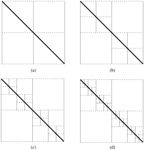
Figure 1: Schematic of bisection of matrix inverses for $d=1$. The broad diagonal line represents the band of the matrix. The narrow vertical lines represent the columns of the matrix inverses $(H-z_{k})^{-1}$ that are calculated. The dashed horizontal lines are rows that are known from the calculated columns due to the matrix being symmetric. These rows then specify boundary conditions for smaller sets of independent linear equations at each sweep (a-d).

Fig. 1 shows a schematic of the RBDM strategy for $d=1$. After the first sweep (Fig 1 (a)) the first, central and last columns are known. From the rows (known as the matrix is symmetric) we now have boundary conditions of two smaller problems which can be solved independently (Fig 1 (b)). We may then bisect these two subproblems in a similar fashion (Fig 1 (c)). The process continues until the dimensions of the submatrices are comparable to the bandwidth of the matrix (Fig 1(d)), and then direct evaluation can be used for the remaining subproblems (smallest blocks on the diagonal in Fig 1(d)).

We now turn to the scaling of the method for $1\geq d\leq 3$. We start with a cubic system and imagine increasing the size of the system by a factor $\gamma$ in $d$ dimensions thereby increasing the total size of the system by $\gamma^{d}$. Firstly, we consider only the cost of the first bisection (Fig 1 (a)) of the system and we consider the DM to have effectively infinite range. To bisect the system into two subsystems requires calculating $n_{\mathrm{col}}$ columns (represented by vertical lines in Fig 1) of the DM and each column requires $\mathcal{O}(N)$ operations to compute. As the system size is increased $\gamma^{(d-1)}n_{\mathrm{col}}$ columns are required to bisect the system. Therefore, the first sweep scales as $\mathcal{O}(N^{(2d-1)/d})$ - and this is the leading term. This bisection operation must then be repeated until all of the desired elements of the DM have been calculated. The number of bisections required goes like $\log_{2^{d}}(N)$. The number of operations required to perform sweep $m$ ($m>1)$ is $\sim N_{1}/2^{(d-1)(m-1)}$ where $N_{1}$ is the number of operations to perform the first sweep. Therefore, the total number of operations may be written as

$$N_{\mathrm{tot}}\propto N^{(2d-1)/d}\sum_{m=0}^{\sim\log_{2^{d}}(N)}\frac{1}{2^{(d-1)(m-1)}}.$$ (6)

For $d=1$ the summation is clearly proportional to $\log_{2}N$. However, in higher dimensions the summation is a convergent series and gives 2 for $d=2$ and $4/3$ for $d=3$. This is an upper bound for the number of operations. Elaborate bisection schemes may reduce the total number of operations but the leading scaling with $N$ will not be affected. Hamiltonians with broader bands from the use of more extended basis functions or non-local pseudopotentials require an increase in $n_{\mathrm{col}}$, however, this does not affect the $N$-scaling.

Another important aspect of any algorithm is numerical stability. As many elements of the DM rely on previous solutions of linear equations we may expect errors to accumulate the more bisections we use. It is difficult to gauge the precise effect on the total energy, however we may concentrate on a single inverse and assume the worst case scenario. If we take one of our shifted matrices that is closest to being singular (the matrix shifted closest to the Fermi energy) $(H-z_{\mathrm{c}})$ then the error in solving for one column of the matrix is proportional to $\epsilon_{\mathrm{m}}\kappa(H-z_{\mathrm{c}})$ where $\epsilon_{\mathrm{m}}$ and $\kappa$ are machine precision and condition of the matrix respectively. At worse we may expect the error to grow linearly with the bisection number, though a random-walk accumulation leading to a square root dependence is more realistic. Fig. 2 shows this slow drift in the value of $Tr(H(H-z_{\mathrm{c}})^{-1})$ where $(H-z_{\mathrm{c}})^{-1}$ is a very ill conditioned matrix (certainly as ill-conditioned as any in a realistic electronic structure calculation). However, each submatrix will have eigenvalue range similar to that of the full matrix but a less clustered eigenspectrum. This will render sub-linear systems becoming further from singularity during the bisection process. The numerics in a full calculation are clearly very complex. One-dimensional model systems were extensively tested in single precision, including double precision iterative improvement of the solutions, from a range of ill-conditioned matrices. In some cases increasing the bisection number produced results closer to that of double precision diagonalization and no catastrophic numerical instabilities were detected.

Figure 2: Relative error in $Tr(H(H-z_{\mathrm{c}})^{-1})$ (single precision) compared to the case where no bisections were used (solid line). The condition of $(H-z_{\mathrm{c}})^{-1}$ is of the order $10^{6}$. For such an ill-conditioned matrix even the relative error in single precision direct diagonalization was $\sim 10^{-5}$. The dashed line shows a fit of the square root of the number of bisections.

As a final example we take a more physically realistic Hamiltonian. A minimal Gaussian basis was used to construct Hamiltonian and overlap matrices for linear C_nH_2n+2 molecules using a norm-conserving non-local pseudopotential Hartwigsen et al. (1998). To obtain a physically reasonable eigenspectrum using the minimal basis for this molecule requires basis functions with a spatial extent which corresponds to the bandwidth of the matrix being approximately 50. This corresponds to a chain length of around 8 carbon atoms before the bandwidth of the matrix becomes less than the dimension of the matrix. For testing purposes a low temperature ($\sim 0.04$eV ) Fermi distribution distribution with $\mu$ taken to be an eigenvalue in the valence band was chosen. This corresponds to a highly charged insulating system with a long range DM (Fig. 3) and also provides an ill-conditioned problem ideal to test numerical stability. The absolute/relative error, compared to direct diagonalization, for the 1001 atom C₃₃₃H₆₆₈ was $\sim 10^{-10}$/$10^{-13}$ and 5 bisections were required. This further puts into context the numerical drift mentioned in the previous section. No iterative improvement was used in this example, only full double precision arithmetic, and the ill-conditioning of the linear systems represents the worst case in a typical calculation. Therefore, in a realistic calculation, chain lengths containing at least one million basis functions in one-dimension (and more in higher dimensions) should be accessible (by which point the natural decay of the density matrix will surely limit the number of required bisections in any case).

Figure 3: Decay of the central column of the density matrix (squares) and two inverses of shifted Hamiltonians for the highly charged C₃₃₃H₆₆₈ system. The Hamiltonian closest to the Fermi energy (crosses) and the Hamiltonian shifted furthest from the real axis (triangles).

We now discuss some further implementation issues. For large systematic basis sets the memory required to store the boundary conditions may become prohibitive - especially in three dimensions. The method can overcome this to some extent by bisecting the system by a factor, $q$, greater than two and building up the density matrix in segments. However, when using large basis sets, a smaller filtered set of basis functions expanded in terms of the underlying basis would be a more realistic approach. It can now be clearly seen how conventional linear algebra can be used for $d=1$ systems. A banded matrix can be $LU$ factorized in $\mathcal{O}(N)$ operations and a linear equation solved in $\mathcal{O}(N)$ using direct methods. Therefore, for $d=1$ iterative algorithms need not be considered - this is useful when using localized basis functions such as Gaussians where iterative methods are still difficult to precondition. Also, the matrices shifted close to $\mu$, at low temperature, become close to singular therefore even basis sets that can be readily preconditioned in a conventional sense (by damping of high kinetic energy components) will also suffer in this regime, so direct methods are desirable. As solving sparse linear systems of equations forms the kernel of the method it is naturally open to any advances in direct sparse solvers for systems where $d>1$.

In principle, a similar procedure can be used if one opts for a polynomial, rather than a rational, approximation to the Fermi function. If $F(H)$ is approximated by a polynomial in $H$, $F(H)\simeq\sum_{k}^{n_{\mathrm{p}}}\omega_{k}H^{k}$, we may construct a set of columns of $H^{k}[k=2,...,n_{\mathrm{p}}]$ and store the necessary boundary matrix elements for each $k$ in a similar fashion to that already described above.

Even if a system has a DM that is sufficiently localized to take advantage of the RBDM method can still be used to dramatically reduce the prefactor if the localization regions are significantly larger than the spatial extent of the basis functions. This will often be the case if highly accurate relative energies are desired. Also, the inverses of Hamiltonians shifted far from the real-axis have more rapid decay allowing true $\mathcal{O}(N)$ evaluation (Fig. 3).

In conclusion, a simple modification of FOE methods has been presented allowing $\mathcal{O}(\alpha(d,N){N^{\frac{2d-1}{d}}})$ scaling where $\alpha(1,N)=\log_{2}(N)$, $\alpha(2,N)\leq 2$ and $\alpha(3,N)\leq 4/3$ without the need for localization. This is a especially useful for systems of low dimensionality with long-ranged DM correlations.

The author thanks S. Goedecker for helpful comments regarding the manuscript and P. R. Briddon for providing the C₃₃₃H₆₆₈ test matrix. This work was supported by the European Commission within the Sixth Framework Programme through NEST-BigDFT (Contract No. BigDFT-511815).

References

- Hohenberg and Kohn (1964) P. Hohenberg and W. Kohn, Phys. Rev. 136, B864 (1964).
- Kohn and Sham (1965) W. Kohn and L. J. Sham, Phys. Rev. 140, A1133 (1965).
- Goedecker (1999) S. Goedecker, Rev. Mod. Phys 71, 1085 (1999).
- Goedecker and Colombo (1994) S. Goedecker and L. Colombo, Phys. Rev. Lett. 73, 122 (1994).
- Goedecker and Teter (1995) S. Goedecker and M. Teter, Phys. Rev. B. 51, 9455 (1995).
- Goedecker (1995) S. Goedecker, J. Comput. Phys. 118, 216 (1995).
- Maslen et al. (1998) P. E. Maslen, C. Ochsenfeld, C. A. White, M. S. Lee, and M. Head-Gordon, J. Phys. Chem. A 102, 2215 (1998).
- Baer and Head-Gordon (1998a) R. Baer and M. Head-Gordon, J. Chem. Phys. 109, 10159 (1998a).
- Baer and Head-Gordon (1998b) R. Baer and M. Head-Gordon, Phys. Rev. B. 58, 15296 (1998b).
- Kenoufi and Polonyi (2004) A. Kenoufi and J. Polonyi, Phys. Rev. B. 70, 205105 (2004).
- Goedecker (1993) S. Goedecker, Phys. Rev. B. 48, 17573 (1993).
- Nicholson and Zhang (1993) D. M. C. Nicholson and X.-G. Zhang, Phys. Rev. B. 56, 12805 (1993).
- Gagel (1998) F. Gagel, J. Comput. Phys. 139, 399 (1998).
- Hartwigsen et al. (1998) C. Hartwigsen, S. Goedecker, and J. Hutter, Phys. Rev. B 58, 3641 (1998).