Thomson scattering from near–solid density plasmas using soft x–ray free electron lasers

Abstract

We propose a collective Thomson scattering experiment at the VUV free electron laser facility at DESY (FLASH) which aims to diagnose warm dense matter at near–solid density. The plasma region of interest marks the transition from an ideal plasma to a correlated and degenerate many–particle system and is of current interest, e.g. in ICF experiments or laboratory astrophysics. Plasma diagnostic of such plasmas is a longstanding issue. The collective electron plasma mode (plasmon) is revealed in a pump–probe scattering experiment using the high–brilliant radiation to probe the plasma. The distinctive scattering features allow to infer basic plasma properties. For plasmas in thermal equilibrium the electron density and temperature is determined from scattering off the plasmon mode.

1 Introduction

Accurate measurements of plasma temperatures and densities are important for understanding and modeling contemporary plasma experiments in the warm dense matter (WDM) regime [1]. WDM is characterized by a free electron density of $n_{e}=10^{21}-10^{26}\,{\rm cm}^{-3}$ and temperatures of several eV. In this regime bound and free electrons become strongly correlated and medium and long–range order are built up. Of special interest is WDM at near–solid density ($n_{e}=10^{21}-10^{22}{\rm cm}^{-3}$, $T_{e}=1-20\,{\rm eV}$) where the transition from an ideal plasma to a degenerate, strongly coupled plasma occurs. In particular, transient plasma behavior at these conditions is observed in dynamical experiments, like laser shock–wave or Z–pinch experiments and are of particular importance for inertial confinement fusion (ICF) experiments. In such applications the plasma evolution follows its path through the largely unknown domain of WDM. Further applications of this plasma domain are found, e.g., in high–energy density physics, astrophysics and material sciences.

A rigorous understanding of highly correlated plasmas is a long–standing and presently unresolved problem. Only recently, with the availability of high–brilliant and coherent VUV and x-ray radiation at a frequency larger than the density dependent electronic plasma frequency $\omega_{pe}$, it became feasible to penetrate through dense plasmas and study basic plasma properties from scattered spectra [2, 3, 4, 5, 6]. The recent effort to develop diagnostic methods using Thomson scattering is an important first step towards a systematic understanding of WDM. Available radiation sources to probe such plasmas are backlighter systems in the x-ray regime as well as free electron laser (FEL) radiation currently available in the VUV. Backlighters have been developed in ICF related research [7] and have been applied to solid density plasmas. The first experiment to measure the spectrally resolved x-ray Thomson scattering spectrum in solid density Be plasma has been reported in [8]. Using the $4.75\,{\rm keV}$ titanium He-$\alpha$ backlighter, the non–collective Thomson scattering spectrum from the thermally distributed electrons allowed the measurement of the Compton–shifted electron distribution function, which was used to determine the plasma density, temperature and ionization degree. A pioneering scattering experiment from the collective electron plasma mode (plasmon) at solid density using a Cl Ly-$\alpha$ backlighter at $2.96\,{\rm keV}$ has been performed recently [9]. A new type of radiation sources for WDM studies became available with the advances of FELs. For instance, the FLASH facility at DESY, has successfully started user experiments in the VUV range $13-50\,{\rm nm}$ [10, 11, 12] using the SASE principle [13, 14]. A proof–of–principle collective Thomson scattering experiment at FLASH ($25\,{\rm nm}$) will be performed in March 2007. This experiment aims to demonstrate Thomson scattering with FEL radiation at near–solid density plasmas as a diagnostic method which is described in this paper in detail. With further advance in FEL technology with respect to bandwidth, photon energy and brilliance, the method presented here can be developed to a standard diagnostic tool for WDM research.

Scattering from ideal plasmas has much been studied [15, 16, 17] and can be described theoretically within the random phase approximation (RPA). It has been shown [5, 6] that in the region of near–solid density collisions significantly modify the scattering spectrum and a theory beyond the RPA is needed. The elaboration of such theories of non–ideal plasmas [18] is more complicated and different ways have been followed in the past. Local field corrections [19], incorporated by Ichimaru [20, 21] using a general density–response formalism, consistently improve the RPA. Alternatively, a theory based on the dielectric function which can be expressed in terms of correlation functions has been studied. For their calculation perturbative methods have been developed [22, 23]. Applications for optical and transport properties in WDM are studied [24, 25, 26].

The paper is organized as follows. In section 2 we outline the theoretical basis for Thomson scattering in WDM, introduce the dynamical structure factor as a central quantity and describe its calculation. Results of the calculations and estimations are used to discuss the applicability of collective Thomson scattering for plasma diagnostics in section 3. In section 4 we describe the planned experiment at FLASH. Based on the results of section 3, we specify out requirements and restrictions relevant for the experiment. In section 5 we give a summary and address future extensions of the method.

2 Theory

2.1 Scattering Geometry

In this section we will outline the theory needed to describe the scattering of coherent radiation from an equilibrium plasma at near–solid density. The scattering geometry is shown in Fig. 1. The plasma is irradiated by the linearly polarized FEL probe–beam in $z$–direction with the polarization pointing into the $x$–direction. The detector is located in the direction of the scattered wave vector ${\bf k}_{f}$ at the distance $R$ much larger than the plasma extension. The direction of ${\bf k}_{f}$ is characterized by the scattering angle $\theta$ and the azimuthal angle $\varphi$ as shown in Fig. 1.

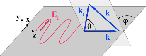
Figure 1: Scattering geometry

The momentum transfer of the scattered photon is given by ${\bf k}={\bf k}_{f}-{\bf k}_{i}$ and its energy transfer by $\omega=\omega_{f}-\omega_{i}$. The modulus of the initial and final wave vector is given by

$$k_{i}=|{\bf k}_{i}|=\frac{\omega_{i}}{c}\sqrt{1-\frac{\omega_{pe}^{2}}{\omega_{i}^{2}}}$$ (1)

$$k_{f}=|{\bf k}_{f}|=\frac{\omega_{f}}{c}\sqrt{1-\frac{\omega_{pe}^{2}}{\omega_{f}^{2}}}\approx\frac{\omega_{f}}{c}\sqrt{1-\frac{\omega_{pe}^{2}}{\omega_{i}^{2}}}~{}.$$ (2)

The square root terms in Eq. (1) and (2) account for the dispersion of incoming and scattered wave. In the density region of $10^{21}-10^{22}\,{\rm cm}^{-3}$ the electron plasma frequency is of the order of $\omega_{pe}=\sqrt{n_{e}e^{2}/\epsilon_{0}m_{e}}\approx 1-4\,{\rm eV}$ and the probe radiation in the VUV–region is of the order of $\omega_{i}\approx\omega_{f}=50-100\,{\rm eV}$. Therefore, we have $|\omega|\lesssim\omega_{pe}\ll\omega_{i}\approx\omega_{f},~{}$ and the approximation in Eq. (2) is well justified. From the scattering geometry given in Fig. 1 one finds for the modulus of the momentum transfer $k=\sqrt{k_{i}^{2}+k_{f}^{2}-2k_{i}k_{f}\cos\theta}$ and using Eqs. (1) and (2)

$$k=\frac{4\pi}{\lambda_{0}}\sin(\theta/2)\,\sqrt{1+\frac{\omega}{\omega_{i}}+\frac{\omega^{2}}{\omega_{i}^{2}}\,\frac{1}{4\sin^{2}(\theta/2)}}\;\sqrt{1-\frac{\omega_{pe}^{2}}{\omega_{i}^{2}}}~{},\quad\omega_{i}=\frac{2\pi c}{\lambda_{0}}~{}.$$ (3)

As pointed out, $|\omega|/\omega_{i}$ and $\omega_{pe}/\omega_{i}$ are small quantities, and it is easily observed from Eq. (3) that the momentum transfer $k$ is well approximated by the relation $k=\frac{4\pi}{\lambda_{0}}\sin(\theta/2)$ for elastic scattering. This, however, is only valid for $\theta>|\omega|/\omega_{i}$, a condition fulfilled in most scattering experiment.

The scattered power $P_{s}$ from the electrons into a frequency interval $d\omega$ and solid angle $d\Omega$ is given by [16]

$$P_{s}(\mathbf{R},\omega)d\Omega d\omega=\frac{P_{i}r_{0}^{2}d\Omega}{2\pi A}\left|\widehat{\mathbf{k}}_{f}\times(\widehat{\mathbf{k}}_{f}\times\widehat{\mathbf{E}}_{0i})\right|^{2}NS(\mathbf{k},\omega)d\omega~{}.$$ (4)

In Eq. (4) $P_{i}$ denotes the incident FEL power, $r_{0}=e^{2}/m_{e}c^{2}=2.8\times 10^{-15}\,{\rm m}$ the classical electron radius, $A$ the plasma area irradiated by the FEL, $N$ the number of nuclei and $S({\bf k},\omega)$ the total electron dynamical structure factor. The polarization term $|\widehat{\mathbf{k}}_{f}\times(\widehat{\mathbf{k}}_{f}\times\widehat{\mathbf{E}}_{0i})|^{2}$ reflects the dependence of the scattered power on the incident laser polarization with the hat denoting unit vectors. For linear polarization and for unpolarized light, respectively, this term is given by

$$\left|\widehat{\mathbf{k}}_{f}\times\left(\widehat{\mathbf{k}}_{f}\times\widehat{\mathbf{E}}_{0i}\right)\right|^{2}=\left\{\begin{array}[]{ll}(1-\sin^{2}\theta\cos^{2}\varphi)&\mbox{lin. polarized}\\[4.30554pt] (1-\frac{1}{2}\sin^{2}\theta)=\frac{1}{2}\left(1+\cos^{2}\theta\right)&\mbox{unpolarized}\end{array}\right.$$ (7)

In the case of linear polarization the dependence on the scattering angle $\theta$ is shown in Fig. 2. The strongest dependence on $\theta$ is observed for $\varphi=0^{\circ}$, whereas at $\varphi=90^{\circ}$ the polarization term is independent of the scattering angle $\theta$.

$\quad\left|\widehat{\mathbf{k}}_{f}\times\left(\widehat{\mathbf{k}}_{f}\times\widehat{\mathbf{E}}_{0i}\right)\right|^{2}$

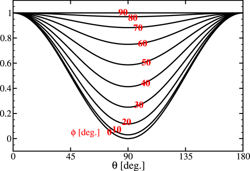
Figure 2: Dependence of the scattered light on laser polarization, scattering angle $\theta$ and azimuthal angle $\varphi$.

As seen from Eq. (4), the scattered power depends on the setup of the scattering experiment (initial probe power, scattering angle, probe wavelength, probe polarization), the density and plasma length, and on the total electron dynamical structure factor $S({\bf k},\omega)$. The dynamical structure factor is the Fourier transform of the electron–electron density fluctuations. It is a central quantity since it contains the details of the correlated many–particle system [21, 27]. The definition and calculation of $S({\bf k},\omega)$ are given in section 2.2.

2.2 Thomson Scattering in WDM

A characterization of plasmas in equilibrium at different densities and temperatures can be performed by simple estimations of dimensionless parameters. The coupling parameter $\Gamma$ is defined as the ratio of the Coulomb energy between two charged particles at a mean particle distance $\bar{d}$ and the thermal energy. Using the Wigner–Seitz radius for $\bar{d}$, we find an expression for the electron coupling parameter

$$\Gamma=\frac{e^{2}}{4\pi\varepsilon_{0}\bar{d}k_{B}T_{e}}\quad,\quad\bar{d}=\left(\frac{4\pi n_{e}}{3}\right)^{-1/3}~{}.$$ (8)

If $\Gamma<1$ the plasma is weakly coupled, and $\Gamma\ll 1$ denotes the ideal plasma regime. Correlations become more important in the coupled plasma regime, where $\Gamma\gtrsim 1$. The degeneracy parameter $\Theta$ estimates the role of quantum statistical effects in the system and is given by the ratio of the thermal energy and the Fermi energy $E_{F}$

$$\Theta=\frac{k_{B}T_{e}}{E_{F}}\quad,\quad E_{F}=\frac{\hbar^{2}}{2m_{e}}\left(3\pi^{2}n_{e}\right)^{2/3}~{}.$$ (9)

In a degenerate plasma, the Fermi energy is larger than the thermal energy, i.e. $\Theta<1$, and most electrons populate states inside the Fermi sea where quantum effects are of importance. Contrary to that, for $\Theta>1$ the role of quantum effects decreases.

The dimensionless scattering parameter $\alpha$ compares the length scale of electron density fluctuations $\ell\approx 2\pi/k$ measured in the scattering experiment to the screening length $\lambda_{sc}$ in the plasma. The scattering parameter is defined as

$$\alpha=\frac{1}{k\lambda_{sc}}\quad,\quad\lambda_{sc}^{-2}\to\lambda_{sc,e}^{-2}=\kappa_{sc,e}^{2}=\frac{e^{2}m_{e}^{3/2}}{\sqrt{2}\pi^{2}\epsilon_{0}\hbar^{3}}\int_{0}^{\infty}dE\,E^{-1/2}f^{e}(E)~{},$$ (10)

where we used the electron screening length $\lambda_{sc,e}$ which is written in terms of the Fermi–Dirac distribution function $f^{e}(E)$ of the electrons and accounts for quantum effects [25]. In the case of a classical Maxwell–Boltzmann electron distribution function, the screening length in Eq. (10) reduces to the Debye screening length $\kappa_{sc,e}^{2}\to\kappa_{D,e}^{2}=n_{e}e^{2}/(\epsilon_{0}k_{B}T_{e})$. For $\alpha>1$, i.e. in the collective scattering regime, only density fluctuations larger than the screening length are observed, while at $\alpha<1$, i.e. in the non-collective scattering regime, the density fluctuations of individual electrons are resolved. As seen from Eq. (3), $\ell=2\pi/k$ is mainly determined by the probe wavelength and the scattering angle (i.e. by the setup of the scattering experiment) while $\lambda_{sc,e}$ is determined by the plasma properties like density and temperature (see Eq. (10)).

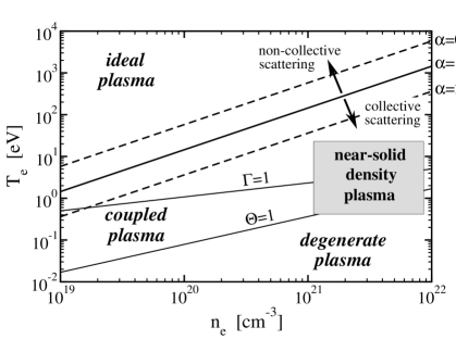
Figure 3: Plasma parameters in the density–temperature plane. The region of moderate temperature, near–solid density plasmas is shown. Also, the electron coupling parameter $\Gamma$, degeneracy parameter $\Theta$ as well as the scattering parameter $\alpha$ is shown as defined in Eqs. (8), (9) and (10). Assumed are the scattering angle $\theta=90^{\circ}$ and probe laser wavelength $\lambda_{0}=25\,{\rm nm}$.

The density–temperature plot in Fig. 3 shows different plasma regions. In particular, the region of moderate temperature and near–solid density (gray region), overlaps with the ideal plasma, coupled plasma and degenerate plasma region. Depending on the scattering geometry conditions and probing wavelength, this plasma region is accessible applying both, collective and non–collective scattering. At a wavelength $\lambda_{0}=25\,{\rm nm}$, however, there is only collective scattering ($\alpha>0$) for arbitrary scattering angle observable from this plasma region.

As outlined in conjunction with Eq. (4), the scattering from the plasma is determined by the mean electron–electron density fluctuations per nucleus which is expressed by the dynamical structure factor $S(\mathbf{k},\omega)$. The structure factor is defined in terms of the electron density response function $\chi_{ee}^{tot}$ via a fluctuation–dissipation theorem (FDT) [28]

$$S({\bf k},\omega)=\frac{\hbar}{n}\,\frac{1}{1-{\rm e}^{-\beta\hbar\omega}}\,{\rm Im}\,\chi_{ee}^{tot}({\bf k},\omega)~{},$$ (11)

with $n$ the number density of the nuclei (atoms and ions). The density response function $\chi_{ee}^{tot}$ is given as [29]

$$\chi_{ee}^{tot}({\bf k},\omega)=\Omega_{0}\,\frac{i}{\hbar}\int_{0}^{+\infty}dt\;{\rm e}^{i(\omega+i\eta)t}\left\langle\left[\delta n_{e}^{tot}({\bf k},t),\delta n_{e}^{tot}(-{\bf k},0)\right]\right\rangle~{},$$ (12)

with $\delta n_{e}^{tot}=n_{e}^{tot}-\langle n_{e}^{tot}\rangle$ being the density fluctuations of all electrons from the average density and the brackets denoting the ensemble average. The normalization volume is denoted by $\Omega_{0}$. The limit $\eta\to 0$ has to be taken after the thermodynamic limit. The solution of Eq. (12) accounting for bound states is a nontrivial problem. Here we follow the idea of Chihara [30, 31] who applied a chemical picture and decomposed the electrons into free and bound electrons of density $n_{e}$ and $n_{e}^{b}$ respectively. With $Z_{f}$ free and $Z_{b}$ bound electrons per nucleus, $n_{e}$ and $n_{e}^{b}$ are related to the ion density $n_{i}$ according to $n_{e}=Z_{f}n_{i}$ and $n_{e}^{b}=Z_{b}n_{i}$. Writing the total electron density $n_{e}^{tot}=n_{e}+n_{e}^{b}$, we can decompose the total density response function in Eq. (12) according to

$$\chi_{ee}^{tot}=\chi_{ff}+\chi_{bb}+\chi_{bf}+\chi_{fb}=\chi_{ff}+\chi_{bb}+2\chi_{bf}~{},$$ (13)

with the electron density response functions of the free–free, bound–bound, bound–free and free-bound system $\chi_{ff}$, $\chi_{bb}$, $\chi_{bf}$ and $\chi_{fb}$, respectively. The response function are defined as in Eq. (12) with the corresponding electron densities. We also used $\chi_{bf}=\chi_{fb}$. Chihara showed that for a classical system the total electron dynamical structure factor can be written in the following decomposed form

$$S(k,\omega) = Z_{f}S_{ee}^{0}(k,\omega)+\left|f_{I}(k)+q(k)\right|^{2}S_{ii}(k,\omega)$$ (14)

$$+Z_{b}\int d\omega^{\prime}\widetilde{S}_{ce}(k,\omega-\omega^{\prime})S_{S}(k,\omega^{\prime})~{}.$$

The first term is due to the free electron fluctuations with $Z_{f}$ the number of free electrons per atom. The second term describes number fluctuations of the weakly and tightly bound electrons, with $f_{I}(k)$ the ion form factor, $q(k)$ the electron screening cloud and $S_{ii}$ the ion–ion structure factor. The last term in Eq. (14) is attributed to inelastic Raman transitions of core electrons into the continuum $\widetilde{S}_{ce}$, modulated with the ion self–motion $S_{S}$.

Under the condition $E_{b}\gg\hbar^{2}k^{2}/(2m)$ [4], where $E_{b}$ is the ionization potential of the bound states, the first two terms in Eq. (14) are most important. For the experimental conditions, specified in section 4, the ionization potential for hydrogen and helium is $E_{b}=13.6\,{\rm eV}$ and $24\,{\rm eV}$, respectively. The energy transferred by the x–ray photons to the bound electrons is only $\sim 0.02\,{\rm eV}$. Therefore, bound–free transitions can be neglected.

2.3 Density Response Function

To shortly review the calculation of the electron density response function we follow [29]. We consider a plasma consisting of free electrons and ions. The electron and the ion response functions in a collision–free one–component plasma (OCP) model are given by the well–known Lindhard expressions

$$\chi_{cc^{\prime}}^{0}({\bf k},\omega)=\delta_{cc^{\prime}}\frac{1}{\Omega_{0}}\sum_{\mathbf{p}}\frac{f_{\mathbf{p}+\mathbf{k}/2}^{c}-f_{\mathbf{p}-\mathbf{k}/2}^{c}}{\Delta E_{\mathbf{p},\mathbf{k}}^{c}-\hbar(\omega+i\eta)}=\chi_{c}^{0}({\bf k},\omega)\delta_{cc^{\prime}}~{},$$ (15)

with $\Delta E_{\mathbf{p},\mathbf{k}}^{c}=E_{\mathbf{p}+\mathbf{k}/2}^{c}-E_{\mathbf{p}-\mathbf{k}/2}^{c}=\hbar^{2}\mathbf{k}\cdot\mathbf{p}/m_{c},$ and the Fermi function $f_{p}^{c}=[\exp(\beta E_{p}^{c}-\beta\mu_{c})+1]^{-1}$ with $\beta=1/(k_{B}T)$. The pole appearing in Eq. (15) is shifted by $\eta$ off the real axis and the limit $\eta\to 0^{+}$ has to be taken after the thermodynamic limit. Eq. (15) is written in matrix form for the plasma species denoted by the indices $c$ and $c^{\prime}$. The matrix is diagonal, i.e. by definition, there are no density fluctuations between different plasma species within the OCP description.

In RPA the plasma interacts via a screened interaction $V_{cc^{\prime}}^{sc}$ obtained self–consistently from the “ring summation” according to

$$V_{cc^{\prime}}^{sc}(\mathbf{k},\omega)=V_{cc^{\prime}}(\mathbf{k})+\sum_{d}V_{cd}(\mathbf{k})\chi_{d}^{0}(\mathbf{k},\omega)\Omega_{0}V_{dc^{\prime}}^{sc}(\mathbf{k},\omega)~{},$$ (16)

which is solved by

$$V_{cc^{\prime}}^{sc}(\mathbf{k},\omega)=\frac{V_{cc^{\prime}}(\mathbf{k})}{1-\chi_{e}^{0}\Omega_{0}V_{ee}-\chi_{i}^{0}\Omega_{0}V_{ii}}$$ (17)

in the case of a Coulomb bare potential, $V_{cc^{\prime}}(k)=e_{c}e_{c^{\prime}}/(\epsilon_{0}\Omega_{0}k^{2})$, considered in this paper only. The screened interaction contains mutual screening contribution from both plasma species (electrons and ions). The RPA response tensor is given by solving

$$\chi_{cc^{\prime}}^{RPA}(\mathbf{k},\omega)=\chi_{c}^{0}(\mathbf{k},\omega)\delta_{cc^{\prime}}+\chi_{c}^{0}(\mathbf{k},\omega)\Omega_{0}V_{cc^{\prime}}^{sc}(\mathbf{k},\omega)\chi_{c^{\prime}}^{0}(\mathbf{k},\omega)$$ (18)

with the matrix elements written as

$$\chi_{ee}^{RPA}({\bf k},\omega) = \frac{\chi_{e}^{0}-\chi_{e}^{0}\Omega_{0}V_{ii}\chi_{i}^{0}}{1-\chi_{e}^{0}\Omega_{0}V_{ee}-\chi_{i}^{0}\Omega_{0}V_{ii}}~{},$$ (19)

$$\chi_{ei}^{RPA}({\bf k},\omega) = \frac{\chi_{e}^{0}\Omega_{0}V_{ei}\chi_{i}^{0}}{1-\chi_{e}^{0}\Omega_{0}V_{ee}-\chi_{i}^{0}\Omega_{0}V_{ii}}~{}.$$ (20)

The remaining two matrix elements are obtained by interchanging $e\leftrightarrow i$.

To take into account the density fluctuations from the bound electrons, not present in Eqs. (19) and (20), one has to solve the dielectric plasma response including bound states [32]. This goes beyond the scope of this paper, and we follow the idea of Chihara [31] by considering the plasma in a chemical picture and decompose the electrons as free, weakly bound and tightly bound electrons. From Eq. (3) we find a maximal momentum transfer at $\omega\approx\omega_{pe}$ for $\theta=180^{\circ}$. Therefore, the smallest length scale $\ell=2\pi/k$ at which density fluctuations can be resolved in the scattering process is $\ell\geq 12\,{\rm nm}$ for a probe wavelength $\lambda_{0}=25\,{\rm nm}$. The electron and ion size is much smaller than $\ell$ and, consequently, details of the atomic structure of the ion enter only in integrated form. This allows to treat the bound electrons in a frozen core approximation. This implies that $\chi_{ff}$, $\chi_{bb}$ and $\chi_{bf}$ for the free–free, bound–bound and bound–free electron density response function respectively can be written as

$$\chi_{ff}^{RPA}({\bf k},\omega) = \chi_{ee}^{RPA}({\bf k},\omega)~{},$$ (21)

$$\chi_{bb}^{RPA}({\bf k},\omega) = Z_{b}^{2}\chi_{ii}^{RPA}({\bf k},\omega)~{},$$ (22)

$$\chi_{bf}^{RPA}({\bf k},\omega) = Z_{b}\chi_{ie}^{RPA}({\bf k},\omega)~{},$$ (23)

where all density fluctuations are referred to the total number of nuclei. From Eq. (13) and (21)–(23) the total electron density response function is written as

$$\chi_{ee}^{tot}({\bf k},\omega)=\chi_{ee}^{RPA}+Z_{b}^{2}\chi_{ii}^{RPA}+2Z_{b}\chi_{ie}^{RPA}~{}.$$ (24)

Upon introduction of the partial dynamical structure factors following Eq. (11)

$$S_{ee}=\frac{\mathcal{C}}{n_{e}}\,{\rm Im}\widetilde{\chi}_{ee}^{RPA}~{},\quad S_{ii}=\frac{\mathcal{C}}{n_{i}}\,{\rm Im}\chi_{ii}^{RPA}~{},\quad S_{ei}=\frac{\mathcal{C}}{\sqrt{n_{e}n_{i}}}\,{\rm Im}\chi_{ei}^{RPA}$$ (25)

with $\mathcal{C}^{-1}=(1-\exp[-\beta\hbar\omega])/\hbar$, we find

$$S=Z_{f}S_{ee}+Z_{b}^{2}S_{ii}+2Z_{b}\sqrt{Z_{f}}S_{ei}~{}.$$ (26)

We made the assumption that the number of nuclei $n$ equals the number of ions $n_{i}$, i.e., there are no neutral atoms in the plasma. Eq. (26) corresponds to the first two terms in Eq. (14). In (14), however, the contribution from the electrons screening the ion charge is separated from $S_{ee}$. This can be done rewriting

$$\chi_{ee}^{RPA} = \widetilde{\chi}_{ee}^{RPA}+\Delta\widetilde{\chi}_{ee}^{RPA}$$ (27)

$$= \frac{\chi_{e}^{0}}{1-\chi_{e}^{0}\Omega_{0}V_{ee}}+\frac{\Omega_{0}^{2}V_{ee}V_{ii}(\chi_{e}^{0})^{2}\chi_{i}^{0}}{\left(1-\chi_{e}^{0}\Omega_{0}V_{ee}-\chi_{i}^{0}\Omega_{0}V_{ii}\right)\left(1-\chi_{e}^{0}\Omega_{0}V_{ee}\right)}$$

$$= \frac{\chi_{e}^{0}}{1-\chi_{e}^{0}\Omega_{0}V_{ee}}+\frac{(\chi_{ei}^{RPA})^{2}}{\chi_{ii}^{RPA}}~{}.$$

In Eq. (27) $\widetilde{\chi}_{ee}^{RPA}$ contains the contributions from the free electrons, whereas $\Delta\widetilde{\chi}_{ee}^{RPA}$ describes the quasi–free electrons which screen the ions. From the Eqs. (22)–(27) we find for the total response function

$$\chi_{ee}^{tot}({\bf k},\omega)=\widetilde{\chi}_{ee}^{RPA}+\left(Z_{b}+\frac{\chi_{ei}^{RPA}}{\chi_{ii}^{RPA}}\right)^{2}\chi_{ii}^{RPA}~{}.$$ (28)

Eq. (28) is a simple model for the total electron response function with tightly and weakly bound electrons “frozen” to the ions. Since we are interested in collective Thomson scattering, i.e. the scattering off electron fluctuations over a distance much larger than the ion size, all atomic details are integrated out. In RPA, Eq. (28) is equivalent to the first two terms in Eq. (14) with $Z_{b}=\lim_{k\to 0}f_{I}(k)$ the integrated charge of the tightly bound electrons.

Beyond the RPA, collisions are considered in the response functions $\chi$ by utilizing the Mermin ansatz [33] which makes use of a relaxation time $\tau$. As outlined in [29, 34] the inclusion of local particle number conservation leads to a generalization of the Mermin ansatz in terms of a complex valued dynamical collision frequency $\tau\to 1/\nu(\omega)$. The collisional response function $\chi_{c}^{\nu,0}$ of plasma species $c$ is then given by

$$\chi_{c}^{\nu,0}(\mathbf{k},\omega)=\left(1-\frac{i\omega}{\nu(\omega)}\right)\left(\frac{\chi_{c}^{0}(\mathbf{k},z)\chi_{c}^{0}(\mathbf{k},0)}{\chi_{c}^{0}(\mathbf{k},z)-\frac{i\omega}{\nu(\omega)}\chi_{c}^{0}(\mathbf{k},0)}\right)$$ (29)

and $z=\omega-{\rm Im}\,\nu(\omega)+i{\rm Re}\,\nu(\omega)$. Eq. (29) is exact in the long wavelength limit and serves as a good approximation for finite $k$. The details of the microscopic calculation of the dynamical collision frequency are reviewed in section 2.4. Having introduced electron–ion collisions for the OCP plasma according to Eq. (29), the equations (19) – (28) can be generalized accordingly and we obtain the total collisional response function $\chi_{cc^{\prime}}^{\nu,tot}$ by simply replacing $\chi_{c}^{0}\to\chi_{c}^{\nu,0}$ in these equations.

2.4 Collision Frequency

As outlined, e.g. in [29, 34], the original Ansatz for the dielectric plasma response made by Mermin [33], can be generalized by calculating the dynamic collisions frequency. In the long–wavelength limit, the dynamical collision frequency can be expressed in terms of the inverse response function via a generalized Drude expression. This inverse response function can be obtained by a perturbative evaluation of the corresponding force–force correlation function with respect to the plasma interaction. The result for the collision frequency in Born approximation can be written as (see [29, 34] for further details)

$$\nu^{\mathrm{Born}}(\omega)=-i\mathcal{K}\frac{n_{i}}{n_{e}\omega}\int_{0}^{\infty}dq\,q^{6}V_{D}^{2}(q)S_{ii}(q)[\epsilon_{\mathrm{RPA}}(q,\omega)-\epsilon_{\mathrm{RPA}}(q,0)]$$ (30)

with $\mathcal{K}=(\epsilon_{0}\Omega_{0}^{2})/(6\pi^{2}e^{2}m_{e}),$ and $S_{ii}(q)$ the static ion–ion structure factor and $V_{D}(q)=-Ze^{2}/(\epsilon_{0}\Omega_{0}(q^{2}+\kappa_{sc,e}^{2}))$ the statically screened Debye potential. The electronic screening length $\kappa_{sc,e}$ is defined in Eq. (10). The electron RPA dielectric function $\epsilon^{RPA}$ in Eq. (30) is related to the Lindhard response function, Eq. (15), according to $\epsilon_{\mathrm{RPA}}^{-1}=1+\chi_{e}^{0}e^{2}/(\epsilon_{0}k^{2}).$ It should be pointed out that the electron screening is accounted for in the Debye potential, whereas ion screening is treated in the ion–ion structure factor according to

$$S_{ii}(q)=\frac{q^{2}}{q^{2}+\kappa_{D,i}^{2}}~{},$$ (31)

with the ion Debye screening length $\kappa_{D,i}^{2}=Z_{f}^{2}n_{i}e^{2}/(\epsilon_{0}k_{B}T_{i}).$ Improvements of $S_{ii}$ which account for ion–ion correlations and screening effects are given, e.g., using pseudo–potentials in hypernetted chain calculations (HNC) [35, 36, 37, 38]. These improvements go beyond the scope of this paper, where we are interested in the electron plasma component only, which is determined by the high–frequency electron collective mode (plasmons). For an improved plasma diagnostics which measures the electron and ion component of the plasma separately from the scattering spectrum, an advanced theory to describe the ion–ion correlations, like HNC, is needed. This is an ultimate requirement if probing nonequilibrium plasma states, e.g., in a two–temperature plasma with $T_{e}\neq T_{i}$.

2.5 Dynamical Structure Factor and Plasma Properties

The dynamical structure factor shows distinct features, which are fingerprints of the plasma properties. Therefore, collective Thomson scattering can be applied as a diagnostic tool as described. The relation of the scattering spectrum (or dynamical structure factor) to the plasma properties is explained in the following.

In Fig. 4 we show a schematic picture of the dynamical structure factor in the collective scattering regime with its characteristic features, the ion feature and the plasmon resonance.

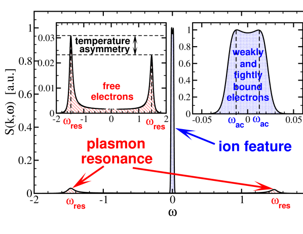
Figure 4: Schematic view of the dynamical structure factor $S(\mathbf{k},\omega)$ as a function of the frequency shift $\omega$ in the collective scattering regime (color online). The high resonance collective mode (plasmons) is shown as a red hatched region. At low frequency shifts, the ion feature due to weakly and tightly bound electrons is shown as the blue dotted region. The plasmon and ion acoustic resonance frequency, $\omega_{res}$ and $\omega_{ac}$, respectively, are shown. The insets on the upper left and right show magnifications of the plasmon resonance and the ion feature respectively.

The asymmetry in the height of the dynamical structure factor at $\pm\omega$ can be explained as follows. The scattering of a photon with initial momentum $\mathbf{k}_{i}$ and frequency $\omega_{i}$ into final momentum $\mathbf{k}_{f}$ and frequency $\omega_{f}$ must be proportional to the probability of the final photon state. Assuming that the system is in thermal equilibrium at a temperature $T$, not disturbed by the laser irradiation, the dynamical structure factor has to be proportional to the Boltzmann factor according to

$$S(\mathbf{k}_{i}\to\mathbf{k}_{f},\omega_{i}\to\omega_{f})\propto\exp\left\{-\frac{\hbar\omega_{f}}{k_{B}T}\right\}~{}.$$ (32)

Similar, for the reverse scattering we have

$$S(\mathbf{k}_{f}\to\mathbf{k}_{i},\omega_{f}\to\omega_{i})\propto\exp\left\{-\frac{\hbar\omega_{i}}{k_{B}T}\right\}~{}.$$ (33)

For a homogeneous and stationary system, the scattering process is described by $\mathbf{k}\equiv\mathbf{k}_{f}-\mathbf{k}_{i}$ and $\omega\equiv\omega_{f}-\omega_{i}$, the momentum and energy transfer, only. From the general property [39] $\chi(\mathbf{k},\omega)=\chi^{\ast}(-\mathbf{k},-\omega)$, we find via the equilibrium FDT (11) and the relations (32), (33)

$$\frac{S(-\mathbf{k},-\omega)}{S(\mathbf{k},\omega)}=\exp\left(-\frac{\hbar\omega}{k_{B}T}\right)~{}.$$ (34)

Eq. (34) is known as detailed balance relation, and it is a general property following from first principles. As seen, the ratio defined in (34) at any particular energy transfer $\hbar\omega$ depends only on the equilibrium temperature of the system. This makes the detailed balance relation a highly suitable tool to measure the temperature of the plasma, independent of any model assumptions other than thermodynamic equilibrium. In Fig. 4 the asymmetry in the dynamical structure factor, denoted as temperature asymmetry, is due to the detailed balance relation.

Scattering from electrons which are weakly or tightly bound to the ions, see discussion in connection with Eq. (14), leads to the low frequency resonance, the ion feature. As shown in Fig. 4, due to the large ion mass, the ion feature shows a very narrow spectral width. Currently, there is no x–ray or VUV radiation available that would allow to spectrally resolve the ion feature. In the future this could be possible with FEL seeding [40] and in recently proposed FELs based on a energy recovery linac scheme with very narrow XUV bandwidth [41].

The high–frequency mode, known as plasmon, is due to the collective scattering from free electrons. In Fig. 4, a red ($\omega<0$) and blue ($\omega>0$) shifted plasmon feature appear due to the creation and annihilation of a plasmon, respectively. Neglecting the plasmon collisional and Landau damping, the plasmon resonance $\omega_{res}$ is approximately given by the plasmon dispersion relation. For a classical collisionless plasma an expression for the plasmon dispersion has been given by Gross and Bohm [42], valid in the long wavelength limit $\hbar k^{2}/(2m_{e}\omega)\ll 1$

$$\omega_{res}^{2}\approx\omega_{pe}^{2}+\frac{3k_{B}T_{e}}{m_{e}}k^{2}~{},$$ (35)

with the density dependent plasma frequency $\omega_{pe}$. The dispersion relation is calculated from the condition ${\rm Re}\,\epsilon(\mathbf{k},\omega)=0$. Eq. (35) follows for a classical Maxwell Boltzmann plasma and the dielectric function $\epsilon$ expanded to order $\mathcal{O}(k^{2})$. An inspection of Eq. (35) reveals immediately that the plasmon resonance position is mainly determined by the plasma frequency and, therefore, by the electron density. The second term in the dispersion relation contains a temperature dependence. Having determined the temperature via the detailed balance relation as explained, the measurement of the plasmon position $\omega_{res}$ provides the free electron density in the plasma.

An improvement of the classical dispersion relation (35) including quantum diffraction is obtained if the electron Lindhard expression for the dielectric function is solved for ${\rm Re}\,\epsilon(\mathbf{k},\omega)=0$. The second moments of the Fermi function are given by Fermi integrals, which can be expressed using an approximate solution [43] to the lowest order in $y=n_{e}\Lambda_{e}^{3}/g_{e}$. Here we have defined the electron thermal wavelength $\Lambda_{e}=h/\sqrt{2\pi m_{e}k_{B}T_{e}}$ and $g_{e}$ the electron spin degeneracy factor. With these approximations an improved dispersion relation (IDR) can be obtained

$$\omega_{res}^{2}(k^{2})\approx\omega_{pe}^{2}+\frac{3k_{B}T_{e}}{m_{e}}k^{2}\left(1+0.088n_{e}\Lambda_{e}^{3}+\ldots\right)+\left(\frac{\hbar k^{2}}{2m_{e}}\right)^{2}~{},$$ (36)

and the ellipsis denoting higher order terms in $y$. This expansion is valid for $y<5.5$ [43]. At the order $\mathcal{O}(k^{4})$ only the leading term is kept. Other terms of the order $\mathcal{O}(k^{4})$ [44] are suppressed by higher moments of the distribution function. It is a simple observation from Eq. (36) that in the limit $\hbar\to 0$ and $n_{e}\Lambda_{e}^{3}\to 0$ the Gross–Bohm dispersion relation, Eq. (35) is recovered. Further, it must be pointed out that both dispersion relations assume ${\rm Im}\,\epsilon(\mathbf{k},\omega)=0$ and, consequently, neglect the effect of collisional damping.

2.6 Continuum Radiation

Independent information on the plasma density and temperature can be obtained from the continuum (bremsstrahlung) emission of the plasma. For demonstration, the emission for an optically thin hydrogen plasma ($Z_{f}=1$) in thermal equilibrium at different temperatures is given by the classical Kramers formula [45, 46]

$$\frac{\mathrm{d}j(\lambda)}{\mathrm{d}V\mathrm{d}\Omega}=\frac{\mathrm{d}P_{b}(\lambda)}{\mathrm{d}V\mathrm{d}\lambda\mathrm{d}\Omega}=\mathcal{C}_{b}\frac{Zg_{ff}n_{e}^{2}e^{6}}{3m_{e}c^{2}\lambda^{2}}\left(\frac{2\pi}{3k_{\mathrm{B}}Tm_{e}}\right)^{1/2}\exp\left(-\frac{2\pi\hbar c}{\lambda k_{\mathrm{B}}T}\right)~{},$$ (37)

with $\mathcal{C}_{b}=2^{5}\pi/(4\pi\epsilon_{0})^{3}$ and $g_{ff}$, the Gaunt factor [47], accounting for quantum and medium corrections. A quantum mechanical calculation of the Gaunt factor [48] showed that $g_{ff}=1$ serves as a good approximation for the spectrum.

3 Results

3.1 Collision Frequency

Using the results of the previous section we can calculate the dynamical structure factor $S(\mathbf{k},\omega)$ via the FDT, Eq. (11), for a collisional hydrogen plasma. The result for the collision frequency calculated in Born approximation according to Eq. (30) is shown in Fig. 5.

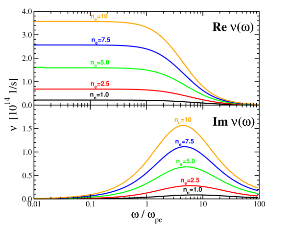
Figure 5: Real and imaginary part of the electron ion dynamical collision frequency in hydrogen as a function of the energy transfer (upper and lower panel respectively). The collision frequency is calculated in Born approximation, Eq. (30), with respect to a statically screened Debye potential. The electron and ion temperature is $12\,{\rm eV}$ and the free electron density $n_{e}$ is given in units of $10^{21}\,{\rm cm}^{-3}$.

It is seen that collsions become more important at higher densities in this domain. This is due to an increasing coupling parameter. At frequencies larger than the plasma frequencies $\omega_{pe}$, the collisions become less effective and the real and imaginary part of the collision frequency goes to zero.

3.2 Dynamical Structure Factor

From the collision frequencies we have calculated the dynamical structure factor using Eqs. (28) with the replacement $\chi_{c}^{0}\to\chi_{c}^{\nu,0}$ for an equilibrium plasma at $T_{e}=T_{i}=12\,{\rm eV}$. The results are plotted in Fig. 6 as a function of the frequency shift $\omega$. Three different FEL probe wavelengths $15\,{\rm nm}$, $25\,{\rm nm}$ and $35\,{\rm nm}$ are shown in the upper, middle and lower panel, respectively. The corresponding momentum transfer $\mathbf{k}$ is calculated from Eq. (3) for a scattering angle of $90^{\circ}$.

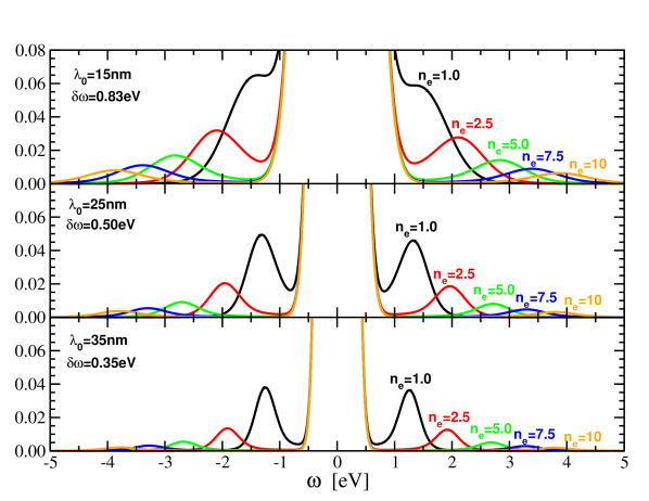
Figure 6: Hydrogen dynamical structure factor $S(k,\omega)$ in units of $1/{\rm eV}$ calculated from Eqs. (26), (29) and (30) including collisions in Born approximation. Each panel shows $S$ for different electron densities $n_{e}$ in units of $10^{21}\,{\rm cm}^{-3}$, at equilibrium conditions $T_{e}=T_{i}=12\,{\rm eV}$, ionization degree $Z_{f}=1$ and a scattering angle of $\theta=90^{\circ}$. For comparison three VUV probe wavelength ($15$, $25$ and $35\,{\rm nm}$) are shown. The finite VUV–bandwidth as well as the spectrometer resolution is accounted for by applying Gaussian convolution with $\delta\omega/\omega_{0}=0.01$ FWHM.

The structure factor is calculated for the same electron densities as in Fig. 5. In order to account for the FEL bandwidth and the final spectrometer resolution, we convoluted the structure factor with a Gaussian profile of $\delta\omega/\omega=0.01$ full width half maximum (FWHM). In Fig. 6 elastic scattering of the bound electrons at $\omega=0$ contributes to the ion feature. Its spectral width is given by the bandwidth and spectrometer resolution. Therefore, the ion feature serves as a measure of the FEL bandwidth. Beside the ion feature we observe the blue and red shifted plasmon resonance. Both resonances are different in height, attributed to the detailed balance relation, Eq. (34). This asymmetry increases with decreasing temperature. In accordance with the Gross–Bohm and the improved dispersion relation, Eqs. (35) and (36), one can observe that the plasmon resonance is shifted to larger resonance frequencies with increasing densities due to an increase of the plasma frequency. Further, in agreement with the plasmon dispersion relation, a larger probe wavelength, leading to a smaller momentum transfer, Eq. (3), yields a smaller plasmon resonance frequency. A calculation of the dynamical structure factor in the density range $10^{21}\,{\rm cm}^{-3}<n_{e}<10^{22}\,{\rm cm}^{-3}$ and a subsequent calculation of the electron density $n_{e}^{GB}$ from the plasmon resonance position via the Gross–Bohm dispersion relation yields a deviation of $(n_{e}^{BG}-n_{e})/n_{e}<0.15$. This deviation is attributed to collisional and quantum effects as well as details of the electron distribution functions, not accounted for in the Gross–Bohm dispersion relation. It should be pointed out that this deviation increases significantly to more than $0.4$ if x–ray scattering is considered at solid densities as, for instance, scattering conditions in [9].

3.3 Continuum Radiation

In order to estimate the sensitivity of the bremsstrahlung emission with respect to the temperature we plot Eq. (37) and its derivative in Fig. 7 for a range of different temperatures. Both panels are normalized at $\lambda=1000\,{\rm nm}$ and are given in arbitrary units.

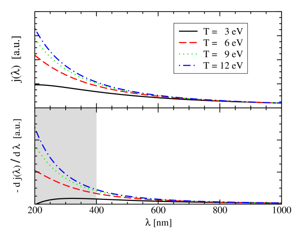
Figure 7: Bremsstrahlung and its negative derivative for a Gaunt factor $g_{ff}=1$ for different temperatures at constant density. Both curves are normalized at $\lambda=1000\,{\rm nm}$ and plotted in arbitrary units.The gray region shows the wavelengths where the spectrum is sensitive to the temperature.

Since we assume no absolute calibration of the spectrum, only the derivative of the spectrum can provide information (lower panel in Fig. 7). The derivative of the spectrum for different temperatures shows deviations at small wavelengths and, consequently, there is a temperature sensitivity of the spectrum present. At small wavelengths the plasma is optically thin and Eq. (37) is applicable. Therefore, measuring the continuum spectrum and fitting the spectrum for a given electron density (measured by collective Thomson scattering) yields an independent estimate of the plasma temperature.

4 Thomson Scattering Experiment at FLASH

To demonstrate the scattering from the collective electron mode of an equilibrium, near–solid density plasma at moderate temperatures $T=1-15\,{\rm eV}$, we propose a proof–of–principle experiment at the VUV free–electron laser FLASH at DESY, Hamburg. The aim of the experiment consists of (i) creating a plasma from a low $Z$ target at near–solid density by an optical heating laser. After a relaxation time in a second step (ii) the plasma is probed by the VUV–FEL and the scattered spectrum is measured by a high resolution transmission grating spectrometer. This novel pump–probe experiment allows to determine basic plasma properties from the distinct features of the scattering spectrum as outlined in the previous sections.

4.1 Experimental Requirements

Based on our results described in section 3, we have analyzed the realization of such an experiment and list some of its most important features:

1. In order to obtain a strong plasmon scattering signal resulting from free electrons and a preferably weak signal from the bound electrons, a low $Z$ target material is used.

2. As the target we employ a cryogenic hydrogen beam which, upon full ionization, provides a free electron density of $n_{e}=(2.2-2.4)\times 10^{22}\,{\rm cm}^{-3}$. After a relaxation time of about $1\,{\rm ps}$ we expect a plasma density of about $n_{e}=10^{21}-10^{22}\,{\rm cm}^{-3}$.

3. Making use of a scattering geometry $\varphi=90^{\circ}$, $\theta=90^{\circ}$ as shown in Fig. 1 and 8, the linear polarization of the FEL pulse does not decrease the scattering spectrum (see Fig. 2). In a temperature range $T_{e}=1-15\,{\rm eV}$ a collective scattering spectrum is expected, as exemplarily shown in Fig. 6 for a temperature of $T_{e}=12\,{\rm eV}$ and various electron densities.

4. Given that the electron density is in the range $n_{e}=10^{21}-10^{22}\,{\rm cm}^{-3}$, FEL radiation at a wavelength of $\lambda_{0}=25\,{\rm nm}$ ($\approx 50\,{\rm eV}$) is chosen in order to fully separate the plasmons from the ion feature. Due to the bandwidth characteristics of the FEL, this cannot be achieved at a smaller wavelength at, e.g. $\lambda_{0}=15\,{\rm nm}$ (see Fig. 6).

5. The application of the detailed balance relation, Eq. (34), for the temperature measurement restricts the plasma temperature to $T_{e}\lesssim 15\,{\rm eV}$. At larger temperatures the asymmetry in the scattering spectrum becomes less than $10\%$ and cannot be resolved experimentally.

6. The number of photons scattered from the plasmons has to be sufficiently high. For a FLASH pulse of energy $E_{FLASH}$ and wavelength $\lambda_{0}$ focused onto the target, one obtains the total number of photons $N_{ph}^{tot}$ by

   $$N_{ph}^{tot}=5.03\times 10^{9}\,E_{FLASH}[\mu{\rm J}]\lambda_{0}[{\rm nm}]~{}.$$ (38)

   The scattered fraction for a plasma length $L$ and the scattering cross section $\sigma=\sigma_{T}/(1+\alpha^{2})\approx\sigma_{T}/\alpha^{2}$ (note: $\alpha>3$) with $\sigma_{T}=6.65\times 10^{-25}\,{\rm cm}^{2}$ the total Thomson cross section, is given by $\sigma n_{e}L$. Neglecting the density correction in the momentum transfer, Eq. (3), we find with Eq. (10) for the scattering parameter $\alpha$

   $$\alpha^{2}=0.1146\;\frac{\lambda_{0}^{2}[{\rm nm}^{2}]n_{e}[10^{21}{\rm cm}^{-3}]}{T_{e}[{\rm eV}]\sin^{2}\theta/2}~{}.$$ (39)

   Therefore, the number of scattered photons $N_{ph}^{sc}$ into the acceptance solid angle of the detector $\Delta\Omega=6\times 10^{-4}\,{\rm sr}$ is given by

   $$N_{ph}^{sc}\approx 1.753\;\frac{E_{FLASH}[\mu{\rm J}]L[\mu{\rm m}]T_{e}[{\rm eV}]}{\lambda_{0}[{\rm nm}]\sin^{2}\theta/2}~{}.$$ (40)

   For a plasma length $L=40\,\mu{\rm m}$, a wavelength $\lambda_{0}=25\,{\rm nm}$, a pulse energy $E_{FLASH}=30\,\mu{\rm J}$, and a scattering angle of $\theta=90^{\circ}$ we find the number of photons collected with the spectrometer $N_{ph}^{sc}\approx 170\,T_{e}{[{\rm eV}]}$.

4.2 Experimental Setup

The vacuum chamber with its main connections being used for the Thomson scattering experiment at DESY and the alignment of the laser beams are shown in Fig. 8 and Fig. 9, respectively.

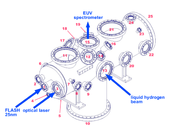
Figure 8: Vacuum chamber with the main connections.

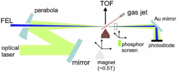
Figure 9: Adjustment of the space and time overlap of the FEL and optical laser.

The plasma is generated by $100\,{\rm fs}$ pulses with up to $10\,{\rm mJ}$ energy at $800\,{\rm nm}$ which are focused to a spot size of $50\,\mu{\rm m}$ in the interaction region where the cryogenic hydrogen beam crosses perpendicularly to the laser beams. For probing the plasma, the FEL beam enters the interaction region through a hole in the parabola mirror, having a beam waist diameter of $20\,\mu{\rm m}$ in the interaction region. Important for the success of the experiment is a good control of the pump–probe–delay between the optical pump laser and the FEL. A parallel alignment of the beams, as shown in Fig. 9, is chosen in order to simplify the coarse adjustment of the temporal overlap using a fast photodiode. For the fine adjustment, the photoelectron (PE) sideband generation technique is applied, which has been successfully demonstrated at FLASH [49] at a helium gas jet. We will use the same laser beam alignment (note: Fig. 9 is taken from [49]) and a similar PE sideband generation setup. In contrast to [49] we apply the technique to the hydrogen gas jet at $100\,{K}$ and record the PE spectrum by a field free electron time–of–flight (TOF) spectrometer. Once the temporal overlap between the optical laser and the FEL has been determined, the the pump–probe delay can be adjusted up to several nanoseconds by a motorized translation stage. The stability of the laser pulse timing is monitored by a streak camera and can be measured on a shot to shot basis by electro–optical sampling [50] with an accuracy of $200\,{\rm fs}$. The repetition rate of the experiment is $5\,{\rm Hz}$, determined by the repetition rate of the FEL.

The hydrogen beam runs perpendicular to the optical laser and the FEL through their joint focus. A cryogenic source similar to the one used here has been characterized for helium at beam diameters of $30-100\,\mu{\rm m}$ [51]. Preparatory tests aiming at a continuous hydrogen beam have been performed at the University of Rostock. Depending on the pressure and temperature conditions, the source provides: a spray of hydrogen droplets, a well collimated beam of droplets or a slow moving filament of solid hydrogen. For the experiment we will make use of the collimated beam consisting of droplets $40\,\mu{\rm m}$ in diameter. It operates stable at a temperature of $T\approx 15\,{\rm K}$ and a pressure of $p\approx 15\,{\rm bar}$ for a nozzle diameter of $d_{nozzle}=20\,\mu{\rm m}$. Similar studies on cryogenic argon beams [52] and piezo-driven hydrogen droplets [53] have been reported.

As shown in Fig. 8, the scattered photons are measured by a high resolution transmission grating EUV spectrometer, mounted perpendicular on top of the interaction region at a scattering angle of $\theta=90^{\circ}$. The spectrometer layout is schematically shown in Fig. 10,

Figure 10: Schematic view of the EUV spectrometer.

details are reported in [54]. A large area transmission grating with a line density of $1000\,{\rm lines/mm}$ will be used. The spectral range is $\lambda=0.5-50\,{\rm nm}$ and the expected spectrum is optimally distributed on the CCD surface (size: $27\times 13.5\,{\rm mm}^{2}$). The spectral resolution of the spectrometer is mainly limited by the dimension of the plasma and the pixel size of the soft x–ray CCD ($13.5\times 13.5\,\mu{\rm m}^{2}$). At the wavelength $\lambda=25\,{\rm nm}$ we expect a resolution of $\Delta\lambda/\lambda\approx 8\times 10^{-3}$. The acceptance solid angle is $\Delta\Omega=6\times 10^{-4}\,{\rm sr}$.

As additional diagnostics an optical spectrometer for the detection of continuum radiation and a CCD–based microscope pointing to the focus will be employed. The microscope is used for characterization of the hydrogen beam in terms of droplet number, size and speed and for initial alignment.

5 Summary

We have shown that x–ray Thomson scattering can be applied as a diagnostic tool to elaborate correlated plasmas in the WDM regime. In particular, we propose a proof–of–principle experiment at the VUV FLASH facility at DESY to measure equilibrium properties of a near–solid density hydrogen plasma. High–brilliant coherent VUV FEL radiation at a wavelength of $\lambda_{0}=25\,{\rm nm}$ will be used to scatter off the dense plasma. The collective Thomson scattering spectrum will be measured using a high resolution, high sensitivity transmission grating EUV-spectrometer. As our theoretical calculations show, the distinctive plasmon features expected in the spectrum, will allow to measure the electron density and temperature. The plasma regime considered in this paper lies in the range of $n_{e}=10^{21}-10^{22}\,{\rm cm}^{-3}$ for the free electron density and $T_{e}=1-15\,{\rm eV}$ for the temperature. A plasma under these conditions is generated by laser irradiation of a cryogenic hydrogen droplet beam. A time delay between the pump and probe laser of the order of the relaxation time ($\approx 1\,{\rm ps}$) will allow to probe the plasma at equilibrium condition.

The electron temperature will be determined by the asymmetry between the red and blue shifted part of the spectrum. This property is directly related to the detailed balance relation which is based on first principles. Therefore, the method provides a reliable measure of the equilibrium temperature. The position of the plasmon resonance is determined by the density. A calculation of the dynamical structure factor for different electron densities allows to identify the plasmon resonance position by the maximum of the plasmon feature. This method provides a reliable electron density measurement if collisional and Landau damping as well as quantum statistical effects are accounted for in the calculations. Estimations for the density can be obtained based on the plasmon dispersion relation with a systematic error of less than $15\%$ in the considered plasma regime. Limiting factors of the proposed measurement have been estimated. The spectral resolution, resulting from the finite FEL bandwidth and EUV–spectrometer resolution, is sufficiently large to spectrally separate the plasmon from the Rayleigh peak. The number of scattered photons off the plasmons has been estimated. More information will be obtained from additional diagnostics. For instance, the measurement of the continuum radiation provides independent information on the plasma density and temperature.

The proposed plasma diagnostic method can be developed into a standard tool for WDM research. Due to the unique features of x-ray and VUV FEL radiation concerning brilliance and coherence, they are favorable sources for Thomson scattering diagnostics which has the potential to be extended to nonequilibrium plasmas in the future. This will need a time–resolved scattering experiment which will reveal the plasma dynamics in WDM and experiments are currently proposed, e.g. at FLASH [55]. The experiment proposed in this paper serves as a precursor to a systematic elaboration of the widely unexplored regime of WDM.

6 Acknowledgments

This work was supported by the virtual institute VH-VI-104 of the Helmholtz association and the Sonderforschungsbereich SFB 652. The work of SHG was performed under the auspices of the U.S. Department of Energy by the University of California Lawrence Livermore National Laboratory under contract number No. W-7405-ENG-48 and the Alexander–von–Humboldt foundation. The work of GG was supported by the Council for the Central Laboratory of the Research Councils (UK).

References

- [1] R.W. Lee, et al., J. Opt. Soc. Am. B 20, 770 (2003).
- [2] D. Riley, et al., Phys. Rev. Lett. 84, 1704 (2000).
- [3] O.L. Landen, et al., J. Quant. Spectrosc. Radiat. Transfer 71, 465 (2001).
- [4] G. Gregori, et al., Phys. Rev. E 67, 026412 (2003).
- [5] A. Höll, et al., Eur. Phys. J. D 29, 159 (2004).
- [6] R. Redmer, et al., IEEE Trans. Plasma Science 33 , 77 (2005).
- [7] O.L. Landen, et al., Rev. Sci. Inst. 72, 627 (2001).
- [8] S.H. Glenzer, et al., Phys. Rev. Lett. 90, 175002 (2003).
- [9] S.H. Glenzer, et al., Phys. Rev. Lett. (2006), submitted.
- [10] V. Ayvazyan, et al., Eur. Phys. J. D. 37, 297 (2006).
- [11] N. Stojanovic, et al., Appl. Phys. Lett., accepted for publication (2006).
- [12] H.N. Chapman et al., Nature Physics Letters, Nov. (2006).
- [13] A. Kondratenko, E. Saldin, Part. Accel. 10, 207 (1980).
- [14] R. Bonifacio, C. Pellegrini, Opt. Commun. 50, 373 (1984).
- [15] T.P. Hughes, Plasma and Laser Light, John Wiley & Sons, NY. (1975).
- [16] J. Sheffield, Plasma Scattering of Electromagnetic Radiation, Academic Press, N.Y. (1975).
- [17] G. Bekefi, Radiation Processes in Plasmas, John Wiley, New York (1966).
- [18] Yu.L. Klimontovich, Kinetic Theory of Nonideal Gases and Nonideal Plasmas, Pergamon, Oxford (1982).
- [19] G. Gregori, et al., J. Phys. A 36 , 5971 (2003).
- [20] S. Ichimaru, et al., Phys. Rev. A32 , 1768 (1985).
- [21] S. Ichimaru, Statistical Plasma Physics, vol. II: Condensed Plasmas, Addison–Wesley (1994).
- [22] G. Röpke, Phys. Rev. E 57, 4673 (1998).
- [23] G. Röpke, A. Wierling, Phys. Rev. E 57, 7075 (1998).
- [24] A. Wierling, et al., Physics of Plasmas 8, 3810 (2001).
- [25] H. Reinholz, Ann. Phys. (Fr) 30, 1 (2005).
- [26] M.W.C. Darma-Wardana, Phys. Rev. E 73, 036401 (2006).
- [27] S. Ichimaru, Plasma Physics: An Introduction to Statistical Physics of Charged Particles, Addison–Wesley (1988).
- [28] R. Kubo, Rep. Prog. Phys. 29, 255 (1966).
- [29] A. Selchow, et al., Phys. Rev. E 64, 056410 (2001).
- [30] J. Chihara, J. Phys. F 17, 295 (1987).
- [31] J. Chihara, J. Phys.: Cond. Matter 12, 231 (2000).
- [32] G. Röpke, R. Der, Phys. Stat. Sol. B 92, 510 (1979).
- [33] N.D. Mermin, Phys. Rev. B 1, 2362 (1970).
- [34] H. Reinholz et al., Phys. Rev. E 62, 5648 (2000).
- [35] P. Seuferling et al., Phys. Rev. A40, 323 (1989).
- [36] Y.V. Arkhipov, A.E. Davletov, Phys. Lett. A 247, 339 (1998).
- [37] G. Gregori, et al., Phys. Rev. E 74, 026402 (2006).
- [38] V. Schwarz, et al., Hypernetted chain calculations for two–component plasmas, Cont. Plasma Phys (2006) submitted.
- [39] A. Sitenko, V. Malnev, Plasma Physics Theory, Chapman & Hall, London (1995).
- [40] J. Feldhaus, et al., Opt. Commun. 140, 341 (1997).
- [41] http://www.4gls.ac.uk
- [42] D. Bohm, E.P. Gross, Phys. Rev. 75, 1851 (1949).
- [43] R. Zimmermann, Many–Particle Theory of Highly Excited Semiconductors, Teubner, Leipzig (1998).
- [44] W.-D. Kraeft, et al., Quantum Statistics of Charged Particle Systems, Akademie-Verlag, Berlin (1986).
- [45] H.A. Kramers, Philos. Mag. 46, 836 (1923).
- [46] G.B. Rybicki, A.P. Lightman, Radiative Processes in Astrophysics, J. Wiley & Sons, New York (1975).
- [47] J.A. Gaunt, Proc. R. Soc. A 126, 654 (1930).
- [48] C. Fortmann, et al., High Energy Density Physics 2, 57 (2006).
- [49] M. Meyer, et al., Phys. Rev A 74, 011401(R) (2006).
- [50] G. Berden, et al., Phys. Rev. Lett. 93, 114802 (2004).
- [51] M.N. Slipchenko, et al., Rev. Sci. Instrum. 73, 3600 (2002).
- [52] M. Grams, et al., Rev. Sci. Instrum. 76, 123904 (2005).
- [53] B. Trostell, Nucl. Instr. Meth. in Phys. Res. A 362, 41 (1995).
- [54] J. Jasny, et al., Rev. Sci. Instrum. 65, 1631 (1994).
- [55] A. Höll, et al., Thomson Scattering Measurements of Plasma Dynamics, FLASH proposal (2006).
- [56] D.N. Zubarev, V. Morozov, G. Röpke, Statistical Mechanics of Nonequilibrium Processes, Akademie Verlag, Berlin (1997).