Cascade Training Technique for Particle Identification

Abstract

The cascade training technique which was developed during our work on the MiniBooNE particle identification has been found to be a very efficient way to improve the selection performance, especially when very low background contamination levels are desired. The detailed description of this technique is presented here based on the MiniBooNE detector Monte Carlo simulations, using both artifical neural networks and boosted decision trees as examples.

,

1 Introduction

Particle identification (PID) is the procedure of selecting signal events while rejecting background events, and is a key step in the data analysis for essentially all particle physics experiments. For some experiments, the search for a possibly very small signal within a large amount of data, such as MiniBooNE, requires an extremely powerful separation of signal from background events.

MiniBooNE [1] is a short baseline accelerator neutrino experiment currently running at the Fermi National Accelerator Laboratory. Its primary goal is to definitely confirm or rule out the potential $\bar{\nu}_{\mu}\to\bar{\nu}_{e}$ oscillation signal claimed by the LSND experiment [2], by looking in the CP-conjugate channel for the $\nu_{e}$ appearance in a $\nu_{\mu}$ beam. The $\nu_{e}$ appearance is identified by the presence of an isolated electron from the charged-current $\nu_{e}C\to e^{-}X$ reaction on the carbon atoms of the mineral oil active medium. In addition to the intrinsic $\nu_{e}$ contamination in the beam, the main backgrounds to the oscillations analysis come from misidentified muons and neutral pions from the $\nu_{\mu}$ quasielastic scattering and neutral-current $\pi^{0}$ production, respectively. In order to reach the design sensitivity, the MiniBooNE PID algorithms must achieve an electron selection efficiency of better than 50%, for an overall background contamination level of approximately 1%.

The crucial points for any PID-based analysis are both the input variables and the underlying algorithm. Each variable must (obviously) have a relatively good separation between signal and background events, while in addition it must yield a good agreement between data and Monte Carlo (MC) in both distributions and correlations. Once the set of PID variables has been identified, the next step is to chose the PID algorithm. In the case in which the signal event statistics are large enough and some few variables already show a very clear separation between signal and background, the simple, straight cuts method may be preferred. Otherwise, the linear or nonlinear combination techniques of the underlying variables, such as Fisher discriminants [3], artificial neural networks (ANN) [4], or boosted decision trees (BDT) [5] should be applied. While ANNs have been relatively widely accepted and successfully used in high energy experimental data analysis in the past decades [6], BDTs as a novel and powerful classification technique have been first introduced to the particle physics community within the MiniBooNE collaboration only recently [7]. Since then it has also been applied to the radiative leptonic decay identification of B-mesons in the BaBar experiment [8], as well as to supersymmetry searches at the LHC [9].

Generally, given a particular set of PID variables and a particular selection algorithm, the maximum PID performance is essentially fixed, up to relatively small variations induced by adjusting some internal settings in the PID code itself, e.g., the learning rate, number of hidden nodes, etc., in the case of neural networks, or the number of leaves, minimum number of events in a leaf, etc., in the case of decision trees. In addition to the PID variables and the algorithm, the training event sets also play a crucial role in the PID performance. Therefore, a careful selection of the training event sample may significantly improve the overall PID performance, as developed within the cascade training technique (CTT) [10].

In this paper, both ANNs and BDTs are taken as examples to describe the cascade training procedure, as based on the MiniBooNE detector MC simulations. In Section 2 we describe briefly the MiniBooNE PID variables used in this study, as well as a systematic procedure for the variable selection. Section 3 describes the cascade training technique, while the results are discussed in Section 4. Our conclusions are summarized in Section 5.

2 PID variable construction and selection

The variable construction and selection is naturally a first concern for an efficient PID. The difference in the information content between signal and background events based on which the separation is made has to be extracted from the variables via some classification algorithm, such as Fisher discriminants, neural networks, decision trees, etc. The variable set used for different experiments and different analysis goals will naturally differ from each other. However, as already mentioned before, some fundamental requirements have to be satisfied, namely: (i) the variable distributions must show some separation between signal and background events, and (ii) the variable distributions and their correlations must show good data/MC agreement. The first requirement is directly connected with the maximum efficiency of the PID, while the second one guarantees the relability of PID output.

The MiniBooNE detector is a spherical steel tank of 610-cm radius, filled with 800 metric tons of ultra-pure mineral oil. An optical barrier divides the detector into an inner region of 575-cm radius, viewed by 1280 photomultiplier tubes (PMT), while the 35-cm-thick outer volume, viewed by 240 PMTs, serves as an active veto shield. Neutrino interactions in the mineral oil are detected via both Cherenkov and scintillation light with a ratio of 3:1 for highly relativistic particles. The particle identification is essentially based on the time and charge distribution recorded at the PMTs.

Every event in the detector is subject to three different maximum-likelihood reconstructions, assuming that the underlying event was an electron, a muon, or a $\pi^{0}$. Ideally, just the $e/\mu$ and $e/\pi$ likelihood ratios should be enough to achieve a powerful separation of the electron signal from the muon and neutral pion backgrounds. However, this is not the case. Therefore, in addition to these two variables, a large set of variables is defined, based on the corrected time at the PMTs and the charge angular distribution with respect to the reconstructed event direction. These variables have been designed to exploit the different topologies of the signal and background events, such as short and fuzzy tracks for electrons, long tracks and sharp rings for muons, two tracks for pions, etc. For any given PMT, at a distance $r_{i}$ from the event vertex, the corrected time $t_{corr}^{(i)}$ is the measured PMT time, $t_{i}$, corrected for the event time, $t_{0}$, and the time of flight:

$$t_{corr}^{(i)}=t_{i}-t_{0}-\frac{r_{i}}{c_{n}},$$

where $c_{n}$ is the speed of light in oil, while $\cos\theta_{i}$ mesures the cosine of the angle between the PMT location and the event direction. By binning the sets of $(t_{corr}^{(i)})$ for the hit PMTs and $(\cos\theta_{i})$ for all PMTs (including the no-hit ones) and recording the hits, charge, time, likelihoods information, etc., in each bin, one can construct several hundreds of potential PID variables. In addition, some reconstructed physical observables, such as the fitted Cherenkov-to-scintillation flux ratio, the event track length, the invariant $\pi^{0}$ mass, etc. can also serve as PID variables, and they are found to be quite powerful.

In principle, all variables which pass the data/MC comparison test can be used as PID input variables. However, it is rather well-known that more input variables does not necessarily imply a better separation in the output, as the PID performance may saturate or even degrade after the number of input variables exceeds a certain limit that depends on the problem itself, as well as the PID algorithm. In the particular case of MiniBooNE, we have found that BDTs can easily handle large numbers of inputs, whereas ANNs appear to be limited to several tens of variables [7]. Therefore, in order to demonstrate the advantage of the cascade training technique, we have decided to limit the number of input variables to some arbitrary small number, e.g., $N_{var}=20$, which can be easily handled by the ANNs. However, the 20 variables used by the ANNs may be different than those used by the BDTs, as we want to utilize a set of inputs that maximizes the performance of that particular algorithm. In the following paragraph we briefly discuss the algorithms for chosing a small subset of input variables from a large pool of input variables.

Boosted decision trees offer several natural ways of ordering the variables and identifying a subset of $N_{var}$ inputs for maximum performance. Once the decision trees have been built with all available variables, the criteria by which the input variables can be easily ordered are, for example: (a) the order in which they are used, (b) the frequency with which they are used, or (c) the number of events they split. Unfortunately, the neural networks do not allow for such a classification. However, an alternative, systematic procedure for ordering the input variables can be defined as follows: starting from the $i$-th variable, scan all other variables and build a neural network or a decision tree using only these two inputs, with the $j$-th variable yielding the best separation. Using variables $(i,j)$, scan again all other variables and search for a third variable, say the $k$-th one, which gives a maximum performance for either a new network or a new decision tree. The procedure is then repeated to find the 4th, 5th, etc., variable, until the desired subset size, $N_{var}$, is reached. Note that starting from different variables may result in a different set of variables for a given final size $N_{var}$, so an additional loop over the first variable is needed.

A direct comparison of the different ordering procedures for BDTs is illustrated in Fig. 1. The three natural variable ordering schemes for BDTs appear to have similar performance for $N_{var}>15$, and they appear to be quite close to saturation at $N_{var}=50$, the maximum value plotted here. The systematic ordering appears to have a slightly better performance than the natural ordering for $N_{var}<20$, in particular when using a relatively low number of inputs. The systematic ordering has been carried out rigurously only to $N_{var}=20$ for computational reasons, as the CPU time increases dramatically with $N_{var}$. The efficiencies displayed here for $20<N_{var}\leq 25$ have been obtained by fixing the first $20$ variables and simply searching for additional new variables, which may not necessarily yield the best efficiencies.

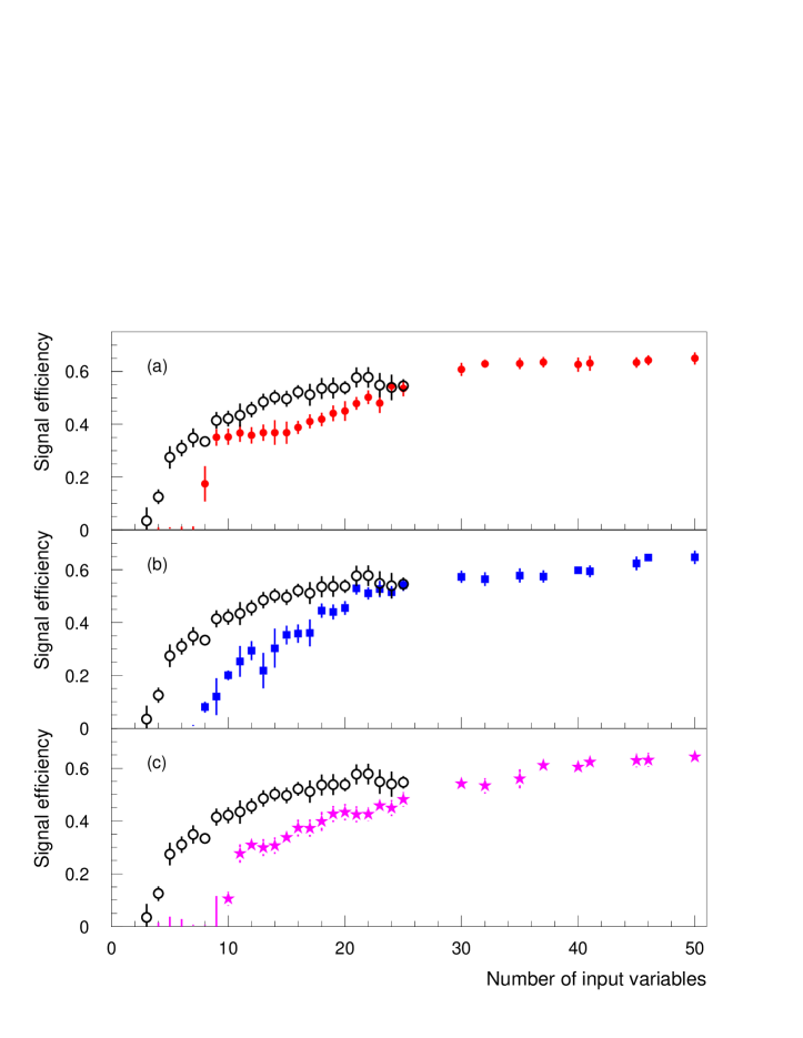
Figure 1: Signal efficiency at 1% background contamination versus number of input variables for boosted decision trees. The variable ordering is by (a) usage ordering, (b) usage frequency, (c) number of events they split, while the systematic ordering – represented by the empty circles – has been superimposed on all of them.

For consistency, we apply this systematic procedure for the variable search to both networks and boosting, using $N_{var}=20$, and turn now to describing the cascade training.

3 The Cascade Training Technique

The idea of the CTT came originally from the combination of the ANN and BDT outputs [11]. In general, the ANN output is not 100% correlated with the BDT output, and hence one can expect some improvement in the overall performance of the PID selection algorithm by combining them together.

Figure 2 below shows the BDT versus the ANN output for the same number of signal and background events. For a 1% background contamination, an ANN cut of about $O_{ANN}>0.98$, or a BDT cut of about $O_{BDT}>1.15$ is necessary. By direct observation it is easy to see that the combined OR region ($O_{ANN}>0.98$ or $O_{BDT}>1.15$) helps improve the signal efficiency relative to a single cut based on either one of the two outputs: the efficiency yields now $62.5\%$, for a slightly higher contamination level of $1.26\%$. Insisting on the nominal background contamination level, a signal efficiency of $54.7\%$ can be reached for $O_{ANN}>0.99$ or $O_{BDT}>1.22$, or even $55.9\%$ for $O_{ANN}>0.92$ and $O_{BDT}>1.03$ by optimizing the cuts.

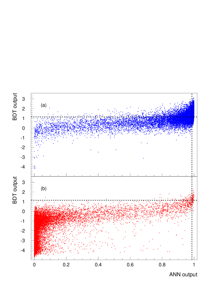
Figure 2: BDT versus ANN output for (a) signal and (b) background events. The vertical and horizontal dashed lines indicate the ANN and BDT cuts for a 1% background contamination, respectively.

There are three ways to combine the ANN and the BDT outputs in a relatively straightforward manner. The first is to optimize the cuts on both of them – as discussed in the previous paragraph. The second is to take them as inputs to another ANN or BDT. The third is to use the output of a single algorithm (either ANN or BDT) as a cut to remove a large portion of the background events, and then force another algorithm to focus on separating the remaining signal and background events – which are now harder to separate. We have found that this latter technique proves to be the most efficient one, especially in the very low background contamination region.

The CTT procedure can be formulated as follows:

1. Prepare three independent sets of samples A, B, and C, where the number of background events in B is several times larger than that in A.
   

2. Train the PID algorithm (ANN or BDT) with sample A, where the input variables may be selected as described in Section 2, if needed.
   

3. Examine the PID output distribution using sample C in order to determine the PID cut value, which is set by the point where the signal and background distributions cross each other, as shown in Fig. 3. The crossing point obviously depends on the relative number of signal and background events in the sample; in this study we have used equal numbers of signal and background events, for both the training and test samples.
   

4. Select the training events from sample B using the PID cut determined by the procedure in step (c) above.
   

5. Train another PID algorithm (ANN or BDT) with the training events obtained in step (d) above, where another variable selection (as described in Section 2) may be applied.
   

6. Test the performance of the resulting PID algorithm with sample C.

Thus, the first ANN or BDT algorithm as built in step (b) only serves to determine the cut used to select the training events for the second PID algorithm training in step (e), and hence the name of the cascade training technique.

4 Results

Figure 3 shows the ANN/BDT output distributions from sample C after the first step training of the two algorithms on sample A. In this particular case the signal/background crossing occurs at $O_{ANN}=0.36$ for neural networks and $O_{BDT}=0$ for the boosted decision trees. Therefore, the events with $O_{ANN}>0.36$ or $O_{BDT}>0$ are selected to form the restricted sample of events, B’ and B”, respectively, used for the second step training. In our case approximately 90% of the signal events pass either one of these cuts, while about 90% of the background events are rejected. Note that the two peaks seen in the BDT output distribution of background events in Fig. 3(b) (dashed histogram) represent the two different bakgrounds in MiniBooNE: the left-most peak around $O_{BDT}=-4$ corresponds to muon events, which are relatively easy to identify, while the right peak at about $O_{BDT}=-1$ corresponds to neutral pion events, which are harder to identify.

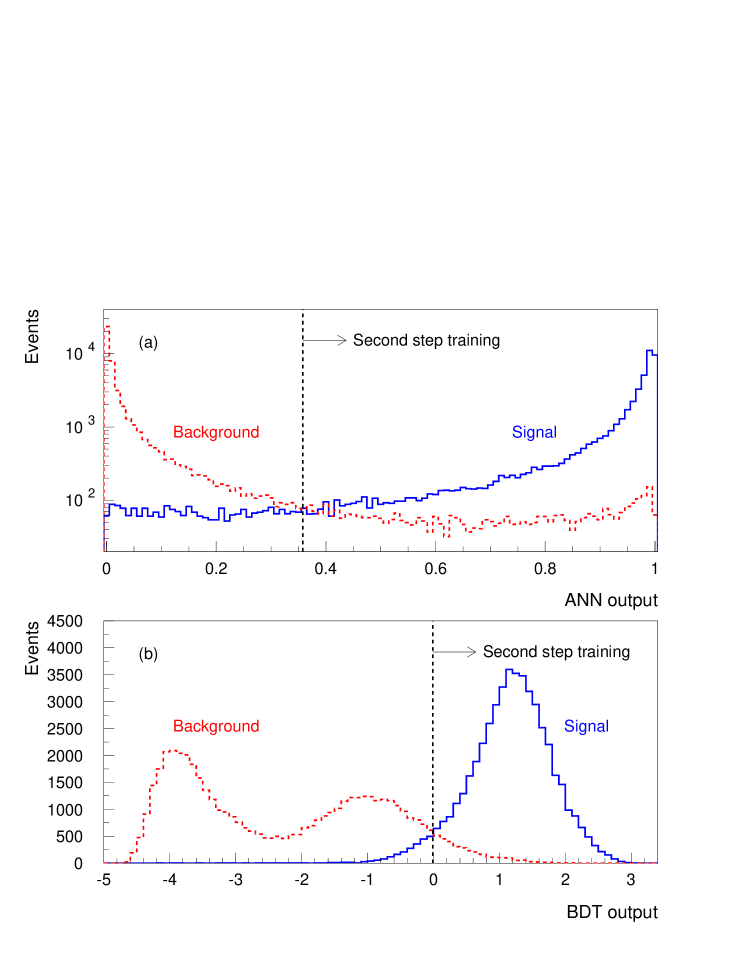
Figure 3: PID output distributions of the test events after the first step training for (a) ANNs and (b) BDTs. The vertical dashed lines indicate the cuts applied to select the training events for the second step training.

The efficiencies of the new ANN and BDT algorithms, trained on the new samples, B’ and B”, respectively, are illustrated in Fig. 4 as a function of the background contamination level, along with the efficiencies of the corresponding algorithms trained on the common sample A. The variable sets used in the first and second step training are identical (although they may be different between ANNs and BDTs).

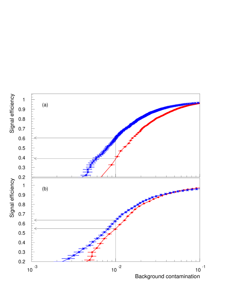
Figure 4: Signal efficiency versus background contamination for (a) ANNs and (b) BDTs for the first and second step training (red circles and blue stars, respectively).

At 1% background contamination, the ANN-based signal efficiency increases from about 39% to 60% after the cascade training, which represents a 50% improvement. This improvement is even more significant at lower background contamination levels, where the signal efficiency can more than double. For boosting however, the improvement by the cascade training appears to be less significant, as it raises the signal efficiency from about 54% to 63% (an improvement of 17%) at 1% background contamination. As in the ANN case, the relative improvement is also more significant at lower levels of contamination.

The lower gain in improvement seen when using boosted decision trees may indicate that the boosting algorithm is already powerful enough to exhaust to a large extent the different information content between signal and background events after the first training step. Nonetheless, while the BDTs may provide a superior PID performance than the conventional ANNs (54% versus 39%), the difference after the CTT is much reduced (63% versus 60%). This implies that the CTT can significantly help the classification algorithms exhaust any useful signal-to-background difference, and push the algorithms to do their best in separating signal from background.

The efficiencies at the 1% contamination level are summarized in Table 1. In addition, the table also gives the efficiencies at a lower contamination level, $0.5\%$, which shows that the relative gains obtained by using the CTT are more significant at lower levels of background contamination.

First	Second	Efficiency (%)	Efficiency (%)
algorithm	algorithm	at 0.5% BCL	at 1.0% BCL
ANN	–	8.4	38.7
ANN	ANN	32.5	60.3
ANN	BDT	39.8	67.6
BDT	–	25.0	54.0
BDT	BDT	37.0	62.8
BDT	ANN	34.2	55.3

Table 1: Signal efficiencies at two different background contamination levels (BCL) for the cascade training after initial selection based on ANNs (top half), and on BDTs (bottom half).

5 Conclusions

In conclusion, a very efficient way to improve ANN- or BDT-based particle identification is introduced, namely the cascade training technique. The procedure is described in detail, as well as the relevant variable construction and selection method.

Our study shows that the CTT can help both ANN and BDT algorithms exhaust the available information contained in the input variables, while significantly improving the PID performance in the low background contamination regions. However, the results reported here are based only on the MiniBooNE detector MC. The relative improvement obtained by the CTT should depend on the concrete experiment/application, variable set, and analysis goal. It could be less, or even more than the numbers presented in this paper.

The intuitive explanation of the high efficiency of CTT may be that if the algorithm can separate hard-to-identify events, it may be able to identify easily separable events quite naturally. Therefore, the strategy is to force the algorithm to focus on learning the different information content from the very signal-like background events and true signal events, while disregarding some number of background-like signal events. Based on our experience, we believe that in general, in multi-component background composition case, the CTT should be a very efficient way to improve the PID efficiency.

Finally, this technique reveals that in addition to the search of good input variables and application of a powerful classification algorithm, an apropriate manipulation of the training event selection opens another way to improve the efficiency of particle identification.

References

- [1] E. Church et al., A proposal for an experiment to measure oscillations and disappearance at FermiLab Booster: BooNE. FERMILAB-P-0898, 1997.
- [2] A. Aguilar et al., Phys. Rev. D64, 112007 (2001).
- [3] G. Cowan, Statistical Data Analysis. Clarendon Press, Oxford (1998). B. Roe, Event Selection Using an Extended Fisher Discriminant Method, PHYSTAT-2003, SLAC, Stanford, CA, September 8–11, 2003.
- [4] http://www.thep.lu.se/ftp/pub/LundPrograms/Jetnet/
- [5] Y. Freund and R. E. Schapire, A Short Introduction to Boosting, Journal of Japanese Society for Artificial Intelligence, 14, 771 (1999). R. E. Schapire, A brief Introduction to Boosting, Proceedings of the Sixteenth International Joint Conference on Artificial Intelligence, 1999. R. Meir and G. Ratsch, An introduction to boosting and leveraging, In S. Mendelson and A. Smola, editors, Advanced Lectures on Machine Learning, LNCS, pages 119-184. Springer, 2003.
- [6] H. Abramowicz, A. Caldwell and R. Sinkus, Nucl. Instrum. Meth. A365, 508 (1995). H. Abramowicz, D. Horn, U. Naftaly and C. Sahar-Pikielny, Nucl. Instrum. Meth. A378, 305 (1996). M. Justice, Nucl. Instrum. Meth. A400, 463 (1997). B. Berg and J. Riedler, Comput. Phys. Commun. 107, 39 (1997). T. Maggipinto, G. Nardulli, S. Dusini, F. Ferrari, I. Lazzizzera, A. Sidoti, A. Sartori and G. P. Tecchiolli, Phys. Lett. B409, 517 (1997). S. Chattopadhyaya, Z. Ahammed, Y. P. Viyogi, Nucl. Instrum. Meth. A421 558 (1999). D0 Collaboration, B. Abbott, et al., Neural Networks for Analysis of Top Quark Production, Fermi-Conf-99-206-E. D0 Collaboration, V. M. Abazov et al., Phys. Lett. B517, 282 (2001). D. V. Bandourin and N. B. Skachkov, JHEP 0404, 007 (2004). S. Forte, L. Garrido, J. I. Latorre and A. Piccione, JHEP 0205, 062 (2002). J. Rojo, JHEP 0605, 040 (2006).
- [7] J. Zhu, H.-J. Yang and B. P. Roe, and Separation in the MiniBooNE Experiment by Using the Boosting Algorithm, MiniBooNE-TN-112, January 9, 2004. B. P. Roe, H.-J. Yang, J. Zhu, Y. Liu, I. Stancu and G. McGregor, Nucl. Instrum. Meth. A 543, 577 (2005).
- [8] I. Narsky, Optimization of Signal Significance by Bagging Decision Trees, physics/0507157.
- [9] J. Conrad and F. Tegenfeldt, Applying Rule Ensembles to the Search for Super-Symmetry at the Large Hadron Collider, JHEP 0607, 040 (2006).
- [10] Y. Liu and I. Stancu, Energy and Geometry Dependence of ParticleID and Cascade Artifical Neural Network and Boosting Training, MiniBooNE-TN-178, March 1, 2006.
- [11] Y. Liu and I. Stancu, The Performance of the S-Fitter Particle Identification, MiniBooNE-TN-141, August 25, 2004.