Basic kinetic wealth-exchange models: common features and open problems

Abstract

We review the basic kinetic wealth-exchange models of Angle [J. Angle, Social Forces 65 (1986) 293; J. Math. Sociol. 26 (2002) 217], Bennati [E. Bennati, Rivista Internazionale di Scienze Economiche e Commerciali 35 (1988) 735], Chakraborti and Chakrabarti [A. Chakraborti, B. K. Chakrabarti, Eur. Phys. J. B 17 (2000) 167], and of Dragulescu and Yakovenko [A. Dragulescu, V. M. Yakovenko, Eur. Phys. J. B 17 (2000) 723]. Analytical fitting forms for the equilibrium wealth distributions are proposed. The influence of heterogeneity is investigated, the appearance of the fat tail in the wealth distribution and the relaxation to equilibrium are discussed. A unified reformulation of the models considered is suggested.

I Introduction

Many scientists have underlined the importance of a quantitative approach in social sciences Bouchaud2005a ; Chatterjee2005b ; Feigenbaum2003a ; Mantegna2000a ; Stauffer2005a ; Stauffer2006c ; Chakrabarti2006a ; Taagepera2008b . In fact, statistical mechanics and social sciences have been always linked to each other in a constructive way, due to the statistical character of the objects of study Ball2002a ; Yakovenko2009a . On one hand, various discoveries, first made in the field of social sciences, introduced new concepts which turned out to be relevant for the development of statistical mechanics and later of the science of complex systems. For instance, fat tails were found by Pareto in the distribution of wealth Pareto1897a ; Pareto1971a_reprint ; the first description of financial time series through statistical mechanics, made by L. Bachelier in his PhD thesis Bachelier1900a ; Bachelier1990b ; Boness1967a , also represents the first formalization of a stochastic process in terms of the random walk model; large fluctuations were observed by Mandelbrot in the time series of cotton price Mandelbrot1963a . On the other hand, physics has often represented a prototype for modelling economic systems. For example, many works of Paul Samuelson were inspired by thermodynamics; the analogies between physics and economics were studied by Jan Tinbergen in his PhD thesis entitled “Minimum Problems in Physics and Economics”. Recent developments of economics rely more and more on the theory of stochastic processes and the science of complex systems Arthur1999a .

The present paper considers some models of wealth exchange between individuals or economical entities, introduced independently in different fields such as social sciences, economics, and physics. We refer to them as kinetic wealth-exchange models (KWEM), since they provide a description of wealth flow in terms of stochastic wealth exchange between agents, resembling the energy transfer between the molecules of a fluid Chatterjee2005b ; Hayes2002a ; Chatterjee2007b . In order to maintain the discussion at a fundamental level, we limit ourselves to the following simple KWEMs: those introduced by Angle (A-models) Angle1983a ; Angle1986a ; Angle2002a ; Angle2006a , Bennati (B-model) Bennati1988a ; Bennati1988b ; Bennati1993a , Chakraborti and Chakrabarti (C-model) Chakraborti2000a , and by Dragulescu and Yakovenko (D-model) Dragulescu2000a . The goal of the paper is to discuss their general common features, formulation, and stationary solutions for the wealth distribution. We consider a heterogeneous KWEM, in order to illustrate how a simple KWEM can generate realistic wealth distributions. We also clarify some relevant issues, recently discussed in the literature, concerning the relaxation to equilibrium and the appearance of a power law tail of the equilibrium distribution in heterogeneous models.

A noteworthy difficulty in the study of wealth or money exchanges based on a kinetic approach had been pointed out by Mandelbrot Mandelbrot1960a :

… there is a great temptation to consider the exchanges of money which occur in economic interaction as analogous to the exchanges of energy which occur in physical shocks between gas molecules… Unfortunately the Pareto distribution decreases much more slowly than any of the usual laws of physics…

The problem referred to in this quotation is that the asymptotic shape of the energy distributions of gases predicted by statistical mechanics usually have the Gibbs form or a form with an exponential tail. The real wealth distributions, instead, exhibit a Pareto power law tail Pareto1897a ; Pareto1971a_reprint ; Levy1997a ; Fujiwara2003a ; Aoyama2003a ,

$$f(x)\sim 1/x^{1+\alpha}\,,$$ (1)

with $1<\alpha<2$. However, it has become clear that (a) the actual shapes of wealth distribution at intermediate values of wealth are well fitted by a $\mathrm{\Gamma}$- or an exponential distribution Angle1986a ; Dragulescu2001a ; Dragulescu2001b ; Ferrero2004a , so that they can be reproduced also by simple KWEMs with homogeneous agents (see Sec. III); (b) KWEMs with suitably diversified agents can generate also the power law tail of the wealth distribution Iglesias2004a ; Chatterjee2005b ; Chatterjee2007b (see Sec. IV). This has opened the way to a simple, quantitative approach in modelling real wealth distributions as arising from wealth exchanges among economical units.

The paper is structured as follows: In Sec. II a general description of a KWEM is given. In Sec. III the homogeneous A-, B-, C, and D-models are discussed. Explicit analytical fitting forms for the equilibrium wealth distributions are given. In Sec. IV we discuss the influence of heterogeneity, taking the heterogeneous C-model as a representative example. In this respect, we analyze the mechanism leading to a robust power law tail. Some issues concerning the convergence time scale of the model and the related finite cut-off of the power law are discussed. In Sec. V a unified reformulation of the A-, C-, and D-models is suggested, which in turn naturally lends itself to further generalizations. An example of generalized model is worked out in detail. Conclusions are drawn in Sec. VI.

II General structure

In the models under consideration the system is assumed to be made up of $N$ agents with wealths $\{x_{i}\geq 0\}$ ($i=1,2,\dots,N$). At every iteration an agent $j$ exchanges a quantity $\Delta x$ with another agent $k$ chosen randomly. The total wealth $X=\sum_{i}x_{i}$ is constant as well as the average wealth $\langle x\rangle=X/N$. After the exchange the new values $x_{j}^{\prime}$ and $x_{k}^{\prime}$ are ($x_{j}^{\prime},x_{k}^{\prime}\geq 0$)

$$x_{j}^{\prime} = x_{j}-\Delta x\,,$$

$$x_{k}^{\prime} = x_{k}+\Delta x\,.$$ (2)

Here, without loss of generality, the minus (plus) sign has been chosen in the equation for the agent $j$ ($k$). The form of the function $\Delta x=\Delta x(x_{j},x_{k})$ defines the underlying dynamics of the model.

In KWEMs, agents can be characterized by an exchange parameter $\omega\in(0,1]$ which defines the maximum fraction of the wealth $x$ that enters the exchange process. Equivalently, one can introduce the saving parameter $\lambda=1-\omega$, with value in the interval $[0,1)$, representing the minimum fraction of $x$ preserved during the exchange. The parameter $\omega$ ($\lambda$) also determines the time scale of the relaxation process as well as the mean value $\langle x\rangle$ at equilibrium Patriarca2007a . If the value of $\omega$ ($\lambda$) is the same for all the agents, the model is referred to as homogeneous (see Sec. III). If the agents assume different values $\omega_{i}$ ($\lambda_{i}$) then the model is called heterogeneous (see Sec. IV). Homogeneous models can reproduce the shape of the $\mathrm{\Gamma}$-distribution observed in real data at small and intermediate values of the wealth. For $\omega<1$ ($\lambda>0$), they have the self-organizing property to converge toward a stable state with a wealth distribution which has a non-zero median, differently from a purely exponential distribution. Models with suitably diversified agents can reproduce also the power law tail (1) found in real wealth distributions.

In actual economic systems the total wealth is not conserved and a more faithful description should be used. It is therefore interesting to observe how the closed economy models considered here, in which $\sum_{i}x_{i}$ is constant, provide realistic shapes of wealth distributions. This suggests that the main factor determining the wealth distribution is the wealth exchange.

When the variation of wealths is not due to an actual exchange between the two agents but the quantity $\Delta x$ is entirely lost by one agent and gained by the other one, the model is called unidirectional. Furthermore, it is possible to conceive multi-agent interaction models, not considered here, in which a number $M>2$ of agents enter each trade. Then the evolution law has the more general form $x_{i}^{\prime}=x_{i}+\Delta x_{i}$, with $i=1,\dots,M$, $\sum_{i=1}^{M}\Delta x_{i}=0$, and the $\Delta x_{i}$ depending somehow on the wealths $x_{i}$ of the $M$ interacting agents.

III Homogeneous models

III.1 A1-model

Here we consider the model introduced by John Angle in 1983 in Refs. Angle1983a ; Angle1986a , referred to as A1-model (a different model of Angle, the One-Parameter Inequality Process, referred to as A2-model, is consider in Sec. III.2 below). The A-models are inspired by the surplus theory of social stratification and describe how a non-uniform wealth distribution arises from wealth exchanges between individuals.

The A1-model is unidirectional and its dynamics is highly nonlinear. The dynamical evolution is determined by Eqs. (2) with $\Delta x$ given as

$$\Delta x=\epsilon\,\omega\,[\eta_{j,k}\,x_{j}-(1-\eta_{j,k})\,x_{k}]\,.$$ (3)

Here $\epsilon$ and $\eta_{j,k}$ are random variables. The first one is a random number in the interval $(0,1)$, which can be distributed either uniformly or with a certain probability distribution $g(\epsilon)$, as in some generalizations of the basic A1-model Angle1983a . The second one is a random dichotomous variable responsible for the unidirectionality of the wealth flow as well as for the nonlinear character of the dynamics. It is a function of the difference between the wealths of the interacting agents $j$ and $k$, $\eta_{j,k}\equiv\phi(x_{k}-x_{j})$, assuming the value $\eta_{j,k}=1$ with probability $p_{0}$ for $x_{j}>x_{k}$ or the value $\eta_{j,k}=0$ with probability $1-p_{0}$ for $x_{k}>x_{j}$. The value $\eta_{j,k}=1$ produces a wealth transfer $|\Delta x|=\epsilon\,\omega\,x_{j}$ from agent $j$ to $k$, while the value $\eta_{j,k}=0$ corresponds to a wealth transfer $|\Delta x|=\epsilon\,\omega\,x_{k}$ from $k$ to $j$.

A special case of the A1-model is that with symmetrical interaction, obtained for $p_{0}=1/2$. Notice that for this value of $p_{0}$ the random variable $\eta_{j,k}\equiv\eta$ becomes independent of $x_{j}$ and $x_{k}$. We have studied this particular case through numerical simulations for various values of the saving parameter $\lambda$. The system considered was made up of $N=10^{5}$ agents with equal initial wealths $x_{0i}^{\,}=1$ and the transactions were performed until equilibrium was reached. The equilibrium distributions in Fig. 1 were obtained by averaging over $10^{5}$ different runs. They are well fitted by the $\mathrm{\Gamma}$-distribution

$$f(x) = \beta\,\gamma_{n}(\beta x)=\frac{\beta}{\Gamma(n)}\,(\beta x)^{n-1}\exp(-\beta x)\,,$$ (4)

where

$$\beta^{-1} = \langle x\rangle/n\,,$$ (5)

$$n \equiv \frac{D}{2}=\frac{1+2\lambda}{2(1-\lambda)}=\frac{3}{2\omega}-1\,.$$ (6)

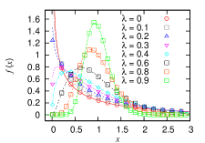
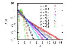
Figure 1: Equilibrium wealth distribution for the basic version of the A1-model defined by Eqs. (3), for the case $p_{0}=1/2$: results of numerical simulations (symbols) and fitting functions Eqs. (4) (curves) for different values of the saving parameter $\lambda=1-\omega$ in linear (above) and semi-log (below) scale. The value of $n$ is governed by Eq. (5). In this simulation the average wealth is $\langle x\rangle=1$.

Since $\lambda=1-\omega\in[0,1)$, the parameter $n$ is a real number in the interval $[1/2,\infty)$. Notice that from Eqs. (4) and (5) it follows that for $n<1$, i.e., for $\lambda<1/4$ ($\omega>3/4$), the $\mathrm{\Gamma}$-distribution diverges for $x\to 0$, as visible in Fig. 1 for the cases $\lambda\!=\!0$, $\lambda\!=\!0.1$, and $\lambda\!=\!0.2$. For the critical value $\lambda=1/4$ ($\omega=3/4$), separating the distributions which diverge from those which go to zero for $x\to 0$, an exponential distribution is obtained,

$$f(x)=\beta\,\gamma_{1}(\beta x)=\beta\exp(-\beta x)\,.$$ (7)

The A1-model has a simple mechanical analogue if the quantity $D=2n$ defined in Eq. (5) is interpreted as an effective dimension for the system and $\beta^{-1}$ as a temperature. It is easy to check that the distribution $\gamma_{n}(\beta x)\equiv\gamma_{D/2}(\beta x)$ given by Eq. (4) is the equilibrium distribution for the kinetic energy of a perfect gas in $D$ dimensions as well as for the potential energy of a $D$-dimensional harmonic oscillator or a general harmonic system with $D$ degrees of freedom. This definition of effective dimension is consistent with the equipartition theorem, since

$$\langle x\rangle=n\,\beta^{-1}=D\beta^{-1}/2\,,$$ (8)

see Ref. Patriarca2004a for details.

III.2 A2-model

The One-Parameter Inequality Process model, here referred to as A2, is another model introduced by John Angle and is described in detail in Refs. Angle2002a ; Angle2006a . It differs from the A1-model considered above in that it only employs a stochastic dichotomic variable $\eta_{jk}$, which can assume randomly the values $\eta_{jk}=0$ or $\eta_{jk}=1$. The model is defined by Eqs. (2) with

$$\Delta x=-\eta_{jk}\omega x_{k}+(1-\eta_{jk})\omega x_{j}\,.$$ (9)

The model describes a unidirectional flow of wealth from agent $k$ toward agent $j$ for $\eta_{jk}=1$ or vice versa for $\eta_{jk}=0$. For the particular case in which the two values of $\eta_{jk}$ are always equiprobable, one can rewrite the process, without loss of generality, with a $\Delta x=\omega x_{k}$ in Eqs. (2). Numerical simulations of this model confirm the findings of Refs. Angle2002a ; Angle2006a , that for small enough $\omega$ the stationary wealth distribution is well fitted by a $\mathrm{\Gamma}$-distribution $\gamma_{n}(x)$, with $n\approx 1/\omega-1=\lambda/(1-\lambda)$. We find that this fitting (not shown) is very good at least up to $\lambda\approx 0.7$.

III.3 B-model

Another KWEM was introduced in 1988 by Eleonora Bennati Bennati1988a ; Bennati1988b . Its basic version, that we discuss here, is a simple unidirectional model where units exchange constant amounts $\Delta x_{0}$ of wealth Bennati1988a ; Bennati1988b ; Bennati1993a . In principle, in the B-model a situation where the wealths of the agents would become negative could occur. This is prevented allowing the transaction to take place only if the condition $x_{j}^{\prime},x_{k}^{\prime}\geq 0$ is fulfilled, i.e., the process is described by Eq. (2) with $\Delta x=\Delta x_{0}$ if $x_{j}^{\prime},x_{k}^{\prime}\geq 0$ and with $\Delta x=0$ otherwise. Since the wealth can vary only by a constant amount $\Delta x_{0}$, the model reminds a set of particles exchanging energy by emitting and re-absorbing light quanta, as illustrated symbolically in Fig. 2.

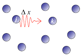
Figure 2: In the B-model the quantity $x$ can only vary by a constant amount $\Delta x=\Delta x_{0}$, which can e.g. be lost by a unit $j$ and then absorbed by a unit $k$, analogously to the emission-absorption process of light quanta of constant frequency.

Analytically the equilibrium state of the B-model is well described by the exponential distribution (7). A main difference respect to the other models considered here is that in the B-model the amount of wealth exchanged between the two agents is independent of $x_{i}$, while in the other models represents a multiplicative random process, since $\Delta x\propto x_{i}$.

III.4 C-model

In the model introduced in 2000 by A. Chakraborti and B. Chakrabarti Chakraborti2000a the general exchange rule reads,

$$x_{j}^{\prime} = \lambda x_{j}+\epsilon\,(1-\lambda)(x_{j}+x_{k})\,,$$

$$x_{k}^{\prime} = \lambda x_{k}+\bar{\epsilon}\,(1-\lambda)(x_{j}+x_{k})\,,$$ (10)

where $\bar{\epsilon}=1-\epsilon$. Here the new wealth $x_{j}^{\prime}$ ($x_{k}^{\prime}$) is expressed as a sum of the saved fraction $\lambda x_{j}^{\prime}$ ($\lambda x_{k}^{\prime}$) of the initial wealth and a random fraction $\epsilon$ ($\bar{\epsilon}$) of the total remaining wealth, obtained summing the respective contributions of agents $j$ and $k$. Equations (10) are equivalent to Eqs. (2), with

$$\Delta x=\omega(\bar{\epsilon}\,x_{j}-\epsilon\,x_{k})=(1-\lambda)(\bar{\epsilon}\,x_{j}-\epsilon\,x_{k})\,.$$ (11)

Like in the A1-model, at equilibrium the system is well described by a $\mathrm{\Gamma}$-distribution (4). For the parameter $n$ we find now Patriarca2004a ; Patriarca2004b

$$n\equiv\frac{D}{2}=\frac{1+2\lambda}{1-\lambda}\,=\frac{3}{\omega}-2\,,$$ (12)

which is twice the value of the corresponding parameter of the A1-model with $p_{0}=1/2$, discussed in Sec. III.1.

In Fig. 3 numerical results are compared with the fitting based on Eq. (12). In this case the probability density is always finite for $x\to 0$, since for $\lambda=0$ ($\omega=1$) one has $n=1$ and the distribution does not diverge, being equal to the exponential function (7).

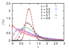
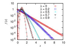
Figure 3: Equilibrium wealth distributions in linear and semi-log scale for different values of the saving parameter $\lambda$ in the closed economy model defined by Eqs. (10). The continuous curves are the fitting functions, i.e. a $\mathrm{\Gamma}$-distribution of the form Eq. (4) just as for the A1-model, but the value of $n(\lambda)$ is given by Eq. (12).

III.5 D-model

The models introduced in 2000 by A. Dragulescu and V. M. Yakovenko Dragulescu2000a were conceived to describe flow and distribution of money. They have a sound interpretation both of the conservation law $x_{j}^{\prime}+x_{k}^{\prime}=x_{j}+x_{k}$, since money is measured in the same unit and conserved during transactions, and of the stochasticity of the update rule, representing a randomly chosen realization of trade. Various models were considered in Ref. Dragulescu2000a , with a $\Delta x$ either constant (similarly to the B-model discussed above) or dependent on the values $x_{i}$ of the agents; also more realistic models, in which e.g. firms were introduced or debts were allowed. For simplicity, we consider among them the model which probably best represents the random character of KWEMs, referred to as the D-model below, in which the total initial amount $x_{j}+x_{k}$ is reshuffled randomly between the two interacting units,

$$x_{j}^{\prime} = \epsilon\,(x_{j}+x_{k})\,,$$

$$x_{k}^{\prime} = \bar{\epsilon}\,(x_{j}+x_{k})\,.$$ (13)

Equivalently, the dynamics can be described by Eqs. (2), with

$$\Delta x=\bar{\epsilon}\,x_{j}-\epsilon\,x_{k}\,.$$ (14)

The D-model is formally recovered from the C-model for $\lambda=0$ ($\omega=1$).

The equilibrium distribution of the D-model is well fitted by the exponential distribution (7). A mechanical analogue of the D-model is a gas, in which particles undergo pair collisions in which some energy is exchanged Whitney1990a , as symbolically illustrated in Fig. 4.

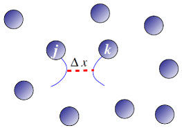
Figure 4: The D-model as well as the C-model prescribe a microscopic interaction between two units analogously to a kinetic model of gas in which, during an elastic collision, two generic particles $j$ and $k$ exchange an energy amount $\Delta x$.

III.6 Stationary wealth distributions

The parameters of the $\mathrm{\Gamma}$-distribution, obtained from the fitting of the wealth distributions of the stationary solutions for the models considered, are summarized in Table 1. The analytical forms of the respective parameters $n$, given as a function of $\omega$ or $\lambda$, provide a good fitting: for the model A2, the fitting is good only up to $\lambda\approx 0.7$. The close analogies among the various models are evident, however the existence of a general solution has not been demonstrated, see e.g. Refs. Repetowicz2005a ; Angle2006a .

Table 1: Comparison of dependence of the fitting parameter $n$ in the $\mathrm{\Gamma}$-distribution (4) on $\lambda$ or $\omega$, for the basic homogeneous versions of the A-, C-, and D-models.

Model	$n(\omega)$	$n(\lambda)$
A1	$3/2\omega\!-\!1$	$(1\!+\!2\lambda)/2(1\!-\!\lambda)$
A2	$1/\omega\!-\!1$	$\lambda/(1\!-\!\lambda)$
C	$3/\omega\!-\!2$	$(1\!+\!2\lambda)/(1\!-\!\lambda)$
D	$1$	$1$

IV Influence of heterogeneity

Here we discuss the influence of heterogeneity, considering as an example the generalization of the C-model. Heterogeneity is introduced by assigning a different parameter $\omega_{i}$ ($\lambda_{i}$) to each agent $i$. The formulation of the heterogeneous models can be straightforwardly obtained from those of the corresponding homogeneous ones by replacing the generic term $\omega\,x_{i}$ ($\lambda x_{i}$) with $\omega_{i}x_{i}$ ($\lambda_{i}x_{i}$) in the evolution law. In the case of the C-model Eqs. (10) become

$$x_{j}^{\prime} = \lambda_{j}x_{j}+\epsilon\,[(1-\lambda_{j})x_{j}+(1-\lambda_{k})x_{k}]\,,$$

$$x_{k}^{\prime} = \lambda_{k}x_{k}+\bar{\epsilon}\,[(1-\lambda_{j})x_{j}+(1-\lambda_{k})x_{k}]\,,$$ (15)

and the exchanged amount of wealth in Eqs. (2) is now

$$\Delta x=\bar{\epsilon}\,\omega_{j}\,x_{j}\!-\!\epsilon\,\omega_{k}\,x_{k}=\bar{\epsilon}(1\!-\!\lambda_{j})x_{j}\!-\!\epsilon(1\!-\!\lambda_{k})x_{k}\,.~{}$$ (16)

The set of parameters $\{\omega_{i}\}$ ($\{\lambda_{i}\}$) is constant in time and specifies the profiles of the agents. The values $\{\omega_{i}\}$ ($\{\lambda_{i}\}$) are assumed to be distributed in the interval between $0$ and $1$ with probabilities $h_{i}$ ($g_{i}$) and $\sum_{i}h_{i}\!=\!1$ ($\sum_{i}g_{i}\!=\!1$). In the limit of an infinite number of agents, one can introduce a probability distribution $h(\omega)$ [$g(\lambda)$], with $\int_{0}^{1}\!d\omega\,h(\omega)\!=\!1$ [$\int_{0}^{1}\!d\lambda\,g(\lambda)\!=\!1$].

Various analytical and numerical studies of this model have been carried out Chatterjee2005b ; Chatterjee2007b ; Angle2002a ; Iglesias2004a ; Repetowicz2005a ; Chatterjee2003a ; Das2003a ; Chatterjee2004a ; Chatterjee2005a ; Das2005a ; Patriarca2005a-brief ; Silva2005a and as a main result it has been found that the exponential law remains limited to intermediate $x$-values, while a Pareto power law appears at larger values of $x$. Such a shape is prototypical for real wealth distributions. Numerical simulations and theoretical considerations suggest that the power law exponent is quite insensitive to the details of the system parameters, i.e., to the distribution $h(\omega)$. In fact, the Pareto exponent depends on the limit $g(\lambda\!\to\!1)$. If $g(\lambda)\sim(1-\lambda)^{\alpha-1}$ with $\lambda\to 1$ and $\alpha\leq 1$, then the corresponding power law has an exponent $\alpha$ Chatterjee2004a . Thus, in general, agents with $\lambda_{i}$ close to $1$ are responsible for the appearance of the power law tail Chatterjee2004a ; Patriarca2005a-brief ; Patriarca2006c .

Probably the most interesting feature of the equilibrium state is that while the shape of the wealth distribution $f_{i}(x)$ of agent $i$ is a $\mathrm{\Gamma}$-distribution, the sum of the wealth distributions of the single agents, $f(x)=\sum_{i}f_{i}(x)$, produces a power law tail. Vice versa, one could say that the global wealth distribution $f(x)$ can be resolved as a mixture of partial wealth probability densities $f_{i}(x)$ with exponential tail, with different parameters. For instance, the corresponding average wealth depends on the saving parameter as $\langle x\rangle_{i}\propto 1/(1-\lambda_{i})=1/\omega_{i}$; see Refs. Bhattacharya2005a-brief ; Patriarca2005a-brief ; Patriarca2006c for details.

Importantly, all real distributions have a finite cutoff; no real wealth distribution has an infinitely extended power law tail. The Pareto law is always observed between a minimum wealth value $x_{\mathrm{min}}$ and a cutoff $x_{\mathrm{max}}$, representing the wealth of the richest agent. This can be well reproduced by the heterogeneous model using an upper cutoff $\lambda_{\rm max}<1$ for the saving parameter distribution $g(\lambda)$: the closer to one is $\lambda_{\rm max}$, the larger is $x_{\mathrm{max}}$ and wider the interval in which the power law is observed Patriarca2006c .

The role of the $\lambda$-cutoff is closely related to and relevant for understanding the relaxation process. The relaxation time scales of single agents in a heterogeneous model are proportional to $1/(1-\lambda_{i})$ Patriarca2007a . This means that the slowest convergence rate is determined by $1-\lambda_{\mathrm{max}}$. In numerical simulations of heterogeneous KWEMs, one necessarily employes a finite $\lambda$-cutoff. However, this should not be regarded as a limit of numerical simulations but a feature suited to describe real wealth distributions. Simulations confirm the fast convergence to equilibrium for each agent with the above mentioned time scale Patriarca2007a . Gupta has demonstrated numerically that the convergence is exponentially fast Gupta2008a .

In Ref. During2008a it has been claimed that heterogeneous KWEMs with randomly distributed $\lambda_{i}$ ($0\leq\lambda_{i}<1$) cannot undergo a fast relaxation toward an equilibrium wealth distribution, but the relaxation should instead take place on algebraic time scale. This in turn means that there cannot exists any power law tail. Such claims are probably correct for systems with a $\lambda$-distribution $g(\lambda)$ rigorously extending as far as $\lambda=1$, corresponding to a power law tail extending as far as $x=\infty$. However, this does not apply to KWEMs with a saving parameter cutoff $\lambda_{\mathrm{max}}<1$, which is the natural choice in describing real systems, as well as in numerical simulations, employing a finite $\lambda$-cutoff: in this case the largest time scale is finite and relaxation is fast.

V Generalizations

In this section a unified reformulation of the exchange laws of the A-, C-, and D-models is suggested and as an example an application to the C-model is made.

V.1 Reformulation

It is possible to reformulate the evolution law either through a single stochastic saving variable $\tilde{\lambda}$ or an equivalent stochastic exchange variable $\tilde{\omega}=1-\tilde{\lambda}$. This formal rearrangement of the equations maintains the form of the evolution law very simple and has at the same time the advantage to be particularly suitable to make further generalizations. For the sake of generality, we consider the case of a heterogeneous system characterized by a parameter set $\{\omega_{i}\}$. The models discussed above (apart from the B-model) can be rewritten according to the basic equations (2), where the wealth exchange term is now given by

$$\Delta x=\tilde{\omega}_{j}\,x_{j}-\tilde{\omega}_{k}\,x_{k}\,.$$ (17)

The meaning of the new stochastic variables $\tilde{\omega}_{j}$ and $\tilde{\omega}_{k}$ introduced is simple: $\tilde{\omega}_{j}$ represents the fraction of wealth given by agent $j$ to $k$ during the transaction, and vice versa for $\tilde{\omega}_{k}$. Comparison with the equations defining the A-, C-, and D-models provides the following definitions for $\tilde{\omega}_{j}$ and $\tilde{\omega}_{k}$:

• In the A1-model, $\tilde{\omega}_{j}$ and $\tilde{\omega}_{k}$ are independent nonlinear stochastic functions of the agent wealths $x_{j}$ and $x_{k}$,

  $$\tilde{\omega}_{j} = \eta_{j,k}\epsilon\,\omega_{j}\,,$$

  $$\tilde{\omega}_{k} = (1-\eta_{j,k})\epsilon\,\omega_{k}\,,$$ (18)

  where $\eta_{j,k}=\phi(x_{k}-x_{j})=1$ with probability $p_{0}$ for $x_{k}-x_{j}>0$ and $\eta_{j,k}=0$ with probability $1-p_{0}$ for $x_{k}-x_{j}<0$, while $\epsilon$ is a random number in $(0,1)$. For $\eta_{j,k}=0$ one has $\tilde{\omega}_{j}=0$ and $\tilde{\omega}_{k}\in(0,\omega_{k})$, whereas for $\eta_{j,k}=1$ one has $\tilde{\omega}_{k}=0$ and $\tilde{\omega}_{j}\in(0,\omega_{j})$.

• In the A2-model, $\tilde{\omega}_{j}$ and $\tilde{\omega}_{k}$ only contain the dichotomic variable,

  $$\tilde{\omega}_{j} = \eta_{j,k}\omega_{j}\,,$$

  $$\tilde{\omega}_{k} = (1-\eta_{j,k})\omega_{k}\,.$$ (19)

• For the C-model,

  $$\tilde{\omega}_{j} = \epsilon\,\omega_{j}\,,~{}~{}~{}~{}~{}~{}~{}~{}~{}~{}~{}~{}~{}~{}~{}\,\!\tilde{\omega}_{j}\in(0,\omega_{j})\,,$$

  $$\tilde{\omega}_{k} = (1-\epsilon)\,\omega_{k}\,,~{}~{}~{}~{}~{}~{}~{}\tilde{\omega}_{k}\in(0,\omega_{k})\,,$$ (20)

  where $\epsilon$ is a random number in $(0,1)$.

• The D-model is recovered from Eqs. (• ‣ V.1) of the C-model when $\omega_{i}=1$ for each agent $i$.

Table 2: Comparison of the A-, C-, and D-models: explicit forms of the random variables $\tilde{\omega}_{j}$ and $\tilde{\omega}_{k}$ in the unified reformulation (17). See text for details.

Model	$\tilde{\omega}_{j}$	$\tilde{\omega}_{k}$
A1	$\epsilon\,\eta\,\omega_{j}$	$(1\!-\!\eta)\epsilon\,\omega_{k}$
A2	$\eta\,\omega_{j}$	$(1\!-\!\eta)\omega_{k}$
C	$\epsilon\,\omega_{j}$	$(1\!-\!\epsilon)\,\omega_{k}$
D	$\epsilon$	$(1\!-\!\epsilon)$

The reformulation is summarized in Table 2 with reference to Eq. (17). Different generalizations can now be done changing only the properties of the stochastic variables $\tilde{\omega}_{i}$, while maintaining the same formulation (17) of the exchange law.

V.2 An example

As an example which can be represented through Eq. (17), we consider a generalization of the homogeneous C-model. In the original version there is a constraint on the maximum fraction of invested wealth, given by a value $0<\omega\leq 1$ of the exchange parameter, or equivalently on the minimum saved fraction, given by a value $0\leq\lambda<1$ of the saving parameter. Now an additional constraint on the minimum fraction of the invested wealth is assumed. This may describe e.g. trades which always have a minimum risk for an agent. It can be represented by an analogous parameter $\omega^{\prime}$, with $0<\omega^{\prime}<\omega$, representing the minimum fraction of wealth invested in a single trade. One can also define a parameter $\lambda^{\prime}=1-\omega^{\prime}$, with $\lambda<\lambda^{\prime}<1$, representing the maximum fraction of saved wealth (i.e. it is not possible to go through a trade without risking a non-zero amount of wealth). Then the stochastic variables $\tilde{\omega}_{i}$ in Eq. (17) become uniform random numbers in intervals defined by the parameters $\omega^{\prime}$ and $\omega$ (or by $\lambda^{\prime}$ and $\lambda$),

$$\tilde{\omega}_{i}\in(\omega^{\prime},\omega)=(1-\lambda^{\prime},1-\lambda)\,.$$ (21)

We have performed numerical simulations for a set of combinations of parameters $(\lambda,\lambda^{\prime})$ and found that the equilibrium distributions are always well fitted by the same $\mathrm{\Gamma}$-distribution (5). However, we have not found a simple analytical formula for fitting the dependence of the parameter $n$ on the saving parameters $\lambda$ and $\lambda^{\prime}$. The behavior of $n$ versus $\lambda$ ($\lambda^{\prime}$) is represented graphically in Fig. 5. Dotted/dashed curves (different colors) represent $n$ versus $\lambda$ for the different fixed values of $\lambda^{\prime}$ shown on the right side These curves stop at $\lambda=\lambda^{\prime}$, since by definition $\lambda<\lambda^{\prime}$. From there the continuous (red) curves start, which represent $n$ versus $\lambda^{\prime}$ for the same fixed values of $\lambda$ listed in the legend on the right. The first (dashed green) curve from the top extending on the whole interval $\lambda=(0,1)$ represents $n$ as a function of $\lambda$ f or $\lambda^{\prime}=1$ and corresponds to the original homogeneous C-model. For this particular case $n(\lambda)$ is known to diverge as $n\sim 1/(1-\lambda)\sim 1/\omega$ for $\lambda\to 1$ (see Table 1), while in all the other cases $n$ is finite.

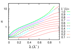
Figure 5: Fitting parameter $n(\lambda,\lambda^{\prime})$ of the $\mathrm{\Gamma}$-distribution $\gamma_{n}(x)$ for the generalized model with $\lambda<\tilde{\lambda}_{i}<\lambda^{\prime}$. Dotted and dashed lines: $n$ as a function of $\lambda$ ($\leq\lambda^{\prime}$ by definition) for fixed values of $\lambda^{\prime}$ shown on the right side. These lines stop at $\lambda=\lambda^{\prime}$ since by definition $\lambda\leq\lambda^{\prime}$. Continuous lines: $n$ as a function of $\lambda^{\prime}$ (($\geq\lambda$) for the same fixed values of $\lambda$ shown on the right side.

VI Conclusions and discussion

We have reviewed some basic KWEMs of closed economy systems, introduced by scientists working in different fields, allowing us to point out analogies and differences between them. We have first considered the homogeneous models and then discussed the influence of heterogeneity. The heterogeneous KWEMs are particularly relevant in the study of real wealth distributions, since they can reproduce both the exponential shape at intermediate values of wealth as well as the power law tail.

In all the models discussed, including the heterogeneous one, the equilibrium wealth distribution of a single agent is well fitted by a $\mathrm{\Gamma}$-distribution, known to be the canonical distribution of a general harmonic system with a suitable number of degrees of freedom. This suggests a simple mechanism underlying the (approach to) equilibrium of these systems, similar to the energy redistribution in a mechanical system. However, a general demonstration that the $\mathrm{\Gamma}$-distribution is the stationary solution of KWEMs and an understanding of how it arises is still missing (see Refs. Repetowicz2005a ; Angle2006a ; ChakraPat2009 ; Anindya2009 for theoretical considerations on and the microeconomic formulation of this issue).

Furthermore, we have discussed how in a heterogeneous KWEM the sum of the single agent wealth distributions can produce a power law tail. In particular, we have clarified some issues concerning the relaxation process and the existence of power law tails: whenever there is a finite cutoff in the saving parameter distribution, the largest time scale of the system is finite and one observes a fast (exponential) relaxation toward a power law, which extends over a finite interval of wealth. The width of such interval depends on saving parameter cutoff.

Due to the similarity of the structures of the models discussed, we have proposed a novel unified reformulation based on the introduction of suitable stochastic variables $\tilde{\omega}_{i}$, representing the actual fraction of wealth lost by the $i$-th agent during a single transaction. This unified formulation lends itself easily to further generalizations, which can be obtained by modifying the stochastic properties of the variable $\tilde{\omega}_{i}$ only, while leaving the general evolution law unchanged. We have illustrated the new formulation by working out in detail an example, in which the fraction of wealth lost $\tilde{\omega}_{i}$ is characterized by a lower as well as an upper limit.

Besides the KWEMs considered in the present paper, originally formulated through finite time difference stochastic equations, other relevant (versions of) KWEMs have been introduced in the literature; see Refs. Lux2005a ; Chatterjee2007b ; Yakovenko2009a for an overview. Their mathematical formulation can be similar to the one of the present paper Angle1986a ; Angle2002a ; Angle2006a ; Iglesias2004a ; Ausloos2007a , or different approaches can be used, such as matrix theory Gupta2006a , the master equation Ispolatov1998a ; Bouchaud2000b ; Ferrero2004a , the Boltzmann equation Slanina2004a ; Repetowicz2005a ; Cordier2005a ; Matthes2007a ; During2007a ; During2008a , the Lotka-Volterra equation Solomon2001a ; Solomon2002a , or Markov chains models Scalas2006b ; Scalas2007a ; Garibaldi2007a . All these models share a description of wealth flow as due to exchanges between basic units. In this respect, they are all very different from the class of models formulated in terms of a Langevin equation for a single wealth variable subjected to multiplicative noise Gibrat1931a ; Mandelbrot1960a ; Levy1996a ; Sornette1998a ; Burda2003a . The latter models can lead to wealth distributions with a power law tail. In fact, they converge toward a log-normal distribution, which, however, does not fit real wealth distributions as well as a $\mathrm{\Gamma}$-distribution or a $\mathrm{\beta}$-distribution and is asymptotically characterized by too large variances Angle1986a .

Finally, we would like to point out that even though KWEMs have been the subject of intensive investigations, their economical interpretation is still an open problem. It is important to keep in mind that in the framework of a KWEM the agents should not be related to the rational agents of neoclassical economics: an interaction between two agents does not represent the effect of decisions taken by two economic agents who have full information about the market and behave rationally in order to maximize their utility. The description of wealth flow provided by KWEMs takes into account the stochastic element, which does not respond by definition to any rational criterion. Also some terms employed in the study of KWEMs, such as saving propensity (replaced here by saving parameter), risk aversion, etc., can be misleading since they seem to imply a decisional aspect behind the behavior of agents. Trying to interpret the dynamics of KWEMs through concepts taken from the neoclassical theory leads to obvious misunderstandings Lux2008a . However, it is interesting to note that very recently, Chakrabarti and Chakrabarti have put forward a microeconomic formulation of the above models, using the utility function as a guide to the behavior of agents in the economy Anindya2009 . Instead, KWEMs provide a description at a coarse grained level, as in the case of many statistical mechanical models, where the connection with the microscopic mechanisms is not visible; however, the equivalence is maintained.

References

- (1)
- (2) J.-P. Bouchaud, The subtle nature of financial random walks, CHAOS 15 (2005) 026104.
- (3) A. Chatterjee, S. Yarlagadda, B. K. Chakrabarti (Eds.), Econophysics of Wealth Distributions - Econophys-Kolkata I, Springer, 2005.
- (4) J. Feigenbaum, Financial physics, Rep. Prog. Phys. 66 (2003) 1611.
- (5) R. N. Mantegna, H. E. Stanley, An Introduction to Econophysics, Cambridge University Press, Cambridge, 2000.
- (6) D. Stauffer, C. Schulze, Microscopic and macroscopic simulation of competition between languages, Phys. Life Rev. 2 (2005) 89.
- (7) D. Stauffer, S. M. de Oliveira, P. M. C. de Oliveira, J. S. de Sa Martins, Biology, Sociology, Geology by Computational Physicists, Elsevier Science, 2006.
- (8) B. K. Chakrabarti, A. Chakraborti, A. Chatterjee (Eds.), Econophysics and Sociophysics: Trends and Perspectives, 1st Edition, Wiley - VCH, Berlin, 2006.
- (9) R. Taagepera, Making social sciences more scientific. The need for predictive models, Oxford University Press, Oxford, 2008.
- (10) P. Ball, The physical modelling of society: a historical perspective, Physica A 314 (2002) 1.
-
(11)
V. Yakovenko, J. J. Barkley Rosser, Statistical mechanics of money, wealth, and
income, arXiv:0905.1518.
URL www.arxiv.org - (12) V. Pareto, Cours d’economie politique, Rouge, Lausanne, 1897.
- (13) V. Pareto, Manual of political economy, Kellag, New York, 1971.
- (14) L. Bachelier, Theorie de la speculation, Annales Scientifiques de l’Ecole Normale Superieure III-17 (1900) 21.
- (15) English translation of: L. Bachelier, Theorie de la speculation, Annales Scientifiques de l’École Normale Superieure (1900) III -17, in: S. Haberman, T. A. Sibbett (Eds.), History of Actuarial Science, Vol. 7, Pickering and Chatto Publishers, London, 1995, p. 15.
- (16) A. J. Boness, English translation of: L. Bachelier, Theorie de la Speculation, Annales de l’Ecole Normale Superieure III-17 (1900), pp. 21-86, in: P. H. Cootner (Ed.), The Random Character of Stock Market Prices, MIT, Cambridge, MA, 1967, p. 17.
- (17) B. B. Mandelbrot, The variation of certain speculative prices, J. Business 36 (1963) 394.
- (18) W. B. Arthur, Science 284 (1999) 107.
- (19) B. Hayes, Follow the money, Am. Sci. 90 (5).
- (20) A. Chatterjee, B. Chakrabarti, Kinetic exchange models for income and wealth distributions, Eur. Phys. J. B 60 (2007) 135.
- (21) J. Angle, The surplus theory of social stratification and the size distribution of personal wealth, in: Proceedings of the American Social Statistical Association, Social Statistics Section, Alexandria, VA, 1983, p. 395.
-
(22)
J. Angle, The surplus theory of social stratification and the size distribution
of personal wealth, Social Forces 65 (1986) 293.
URL http://www.jstor.org - (23) J. Angle, The statistical signature of pervasive competition on wage and salary incomes, J. Math. Sociol. 26 (2002) 217.
- (24) J. Angle, The inequality process as a wealth maximizing process, Physica A 367 (2006) 388.
- (25) E. Bennati, La simulazione statistica nell’analisi della distribuzione del reddito: modelli realistici e metodo di Monte Carlo, ETS Editrice, Pisa, 1988.
- (26) E. Bennati, Un metodo di simulazione statistica nell’analisi della distribuzione del reddito, Rivista Internazionale di Scienze Economiche e Commerciali 35 (1988) 735.
- (27) E. Bennati, Il metodo Monte Carlo nell’analisi economica, Rassegna di lavori dell’ISCO X (1993) 31.
- (28) A. Chakraborti, B. K. Chakrabarti, Statistical mechanics of money: How saving propensity affects its distribution, Eur. Phys. J. B 17 (2000) 167.
- (29) A. Dragulescu, V. M. Yakovenko, Statistical mechanics of money, Eur. Phys. J. B 17 (2000) 723.
- (30) B. Mandelbrot, The Pareto-Levy law and the distribution of income, Int. Econ. Rev. 1 (1960) 79.
- (31) M. Levy, S. Solomon, New evidence for the power-law distribution of wealth, Physica A 242 (1997) 90.
- (32) Y. Fujiwara, W. Souma, H. Aoyama, T. Kaizoji, M. Aoki, Growth and fluctuations of personal income, Physica A 321 (2003) 598.
- (33) H. Aoyama, W. Souma, Y. Fujiwara, Growth and fluctuations of personal and company’s income, Physica A 324 (2003) 352.
- (34) A. Dragulescu, V. M. Yakovenko, Exponential and power-law probability distributions of wealth and income in the United Kingdom and the United States, Physica A 299 (2001) 213.
- (35) A. Dragulescu, V. M. Yakovenko, Evidence for the exponential distribution of income in the usa, Eur. Phys. J. B 20 (2001) 585.
- (36) J. C. Ferrero, The statistical distribution of money and the rate of money transference, Physica A 341 (2004) 575.
- (37) J. R. Iglesias, S. Goncalves, G. Abramsonb, J. L. Vega, Correlation between risk aversion and wealth distribution, Physica A 342 (2004) 186.
- (38) M. Patriarca, A. Chakraborti, E. Heinsalu, G. Germano, Relaxation in statistical many-agent economy models, Eur. J. Phys. B 57 (2007) 219.
- (39) M. Patriarca, A. Chakraborti, K. Kaski, Statistical model with a standard gamma distribution, Phys. Rev. E 70 (2004) 016104.
- (40) M. Patriarca, A. Chakraborti, K. Kaski, Gibbs versus non-Gibbs distributions in money dynamics, Physica A 340 (2004) 334.
- (41) C. A. Whitney, Random processes in physical systems. An introduction to probability-based computer simulations, Wiley Interscience, NY, 1990.
- (42) P. Repetowicz, S. Hutzler, P. Richmond, Dynamics of money and income distributions, Physica A 356 (2005) 641.
- (43) A. Chatterjee, B. K. Chakrabarti, S. S. Manna, Money in gas-like markets: Gibbs and Pareto laws, Physica Scripta T 106 (2003) 367.
-
(44)
A. Das, S. Yarlagadda, A distribution function analysis of wealth distribution.
URL arxiv.org:cond-mat/0310343 - (45) A. Chatterjee, B. K. Chakrabarti, S. S. Manna, Pareto law in a kinetic model of market with random saving propensity, Physica A 335 (2004) 155.
- (46) A. Chatterjee, B. K. Chakrabarti, R. B. Stinchcombe, Master equation for a kinetic model of trading market and its analytic solution, Phys. Rev. E 72 (2005) 026126.
- (47) A. Das, S. Yarlagadda, An analytic treatment of the Gibbs–Pareto behavior in wealth distribution, Physica A 353 (2005) 529.
- (48) M. Patriarca, A. Chakraborti, K. Kaski, G. Germano, Kinetic theory models for the distribution of wealth: Power law from overlap of exponentials, in Ref. Chatterjee2005b p.93.
- (49) A. C. Silva, V. M. Yakovenko, Temporal evolution of the ‘thermal’ and ‘superthermal’ income classes in the usa during 1983-2001, Europhysics Letters 69 (2005) 304.
- (50) M. Patriarca, A. Chakraborti, G. Germano, Influence of saving propensity on the power law tail of wealth distribution, Physica A 369 (2006) 723.
- (51) K. Bhattacharya, G. Mukherjee, S. S. Manna, Detailed simulation results for some wealth distribution models in econophysics, in Ref. Chatterjee2005b p.111.
- (52) A. K. Gupta, Relaxation in the wealth exchange models, Physica A 387 (2008) 6819.
- (53) B. Düring, D. Matthes, G. Toscani, Kinetic equations modelling wealth redistribution: A comparison of approaches, Phys. Rev. E 78 (2008) 056103.
-
(54)
A. Chakraborti and M. Patriarca, A variational principle for the Pareto law,
arXiv:cond-mat/0605325v2 (2008).
URL www.arxiv.org - (55) A-S. Chakrabarti, B. K. Chakrabarti, Physica A, 388 (2009) 4151.
- (56) T. Lux, Emergent statistical wealth distributions in simple monetary exchange models: A critical review, in: A. Chatterjee, S.Yarlagadda, B. K. Chakrabarti (Eds.), Econophysics of Wealth Distributions, Springer, 2005, p. 51.
- (57) M. Ausloos, A. Pekalski, Model of wealth and goods dynamics in a closed market, Physica A 373 (2007) 560.
- (58) A. K. Gupta, Money exchange model and a general outlook, Physica A 359 (2006) 634.
- (59) S. Ispolatov, P. L. Krapivsky, S. Redner, Wealth distributions in asset exchange models, Eur. Phys. J. B 2 (1998) 267.
- (60) J. P. Bouchaud, M. Mezard, Wealth condensation in a simple model of economy, Physica A 282 (2000) 536.
- (61) F. Slanina, Inelastically scattering particles and wealth distribution in an open economy, Phys. Rev. E 69 (2004) 046102.
- (62) S. Cordier, L. Pareschi, G. Toscani, On a kinetic model for a simple market economy, J. Stat. Phys. 120 (2005) 253.
- (63) D. Matthes, G. Toscani, On steady distributions of kinetic models of conservative economies, J. Stat. Phys. 130 (2007) 1087.
- (64) B. Düring, G. Toscani, Hydrodynamics from kinetic models of conservative economies, Physica A 384 (2007) 493.
- (65) S. Solomon, P. Richmond, Power laws of wealth, market order volumes and market returns, Physica A 299 (2001) 188.
- (66) S. Solomon, P. Richmond, Stable power laws in variable economies; Lotka-Volterra implies Pareto-Zipf, Eur. Phys. J. B 27 (2002) 257.
- (67) E. Scalas, U. Garibaldi, S. Donadio, Statistical equilibrium in simple exchange games I, Eur. Phys. J. B 53 (2006) 267.
- (68) E. Scalas, U. Garibaldi, S. Donadio, Erratum. Statistical equilibrium in simple exchange games I, Eur. Phys. J. B 60 (2007) 271.
- (69) U. Garibaldi, E. Scalas, P. Viarengo, Statistical equilibrium in simple exchange games II. the redistribution game, Eur. Phys. J. B 60 (2007) 241.
- (70) R. Gibrat, Les Inégalités Economiques, Sirey, 1931.
- (71) M. Levy, S. Solomon, Power laws are logarithmic Boltzmann laws, Int. J. Mod. Phys. C 7 (1996) 595.
- (72) D. Sornette, Multiplicative processes and power laws, Phys. Rev. E 57 (1998) 4811.
- (73) Z. Burda, J. Jurkiewics, M. A. Nowak, Is Econophysics a solid science?, Acta Physica Polonica B 34 (2003) 87.
- (74) T. Lux, Applications of statistical physics in finance and economics, Kiel Working Paper 1425.