Steric effects in the dynamics of electrolytes at large applied voltages:
II. Modified Poisson-Nernst-Planck equations

Abstract

In situations involving large potentials or surface charges, the Poisson Boltzman(PB) equation has shortcomings because it neglects ion-ion interactions and steric effects. This has been widely recognized by the electrochemistry community, leading to the development of various alternative models resulting in different sets ”modified PB equations”, which have had at least qualitative success in predicting equilibrium ion distributions. On the other hand, the literature is scarce in terms of descriptions of concentration dynamics in these regimes. Here, adapting strategies developed to modify the PB equation, we propose a simple modification of the widely used Poisson-Nernst-Planck (PNP) equations for ionic transport, which at least qualitatively accounts for steric effects. We analyze numerical solutions of these MPNP equations on the model problem of the charging of a simple electrolyte cell, and compare the outcome to that of the standard PNP equations. Finally, we repeat the asymptotic analysis of Bazant, Thornton, and Ajdari Bazant et al. (2004) for this new system of equations to further document the interest and limits of validity of the simpler equivalent electrical circuit models introduced in Part I for such problems.

I Introduction

In Part I of this series, we focused on steric effects of finite ion size on the charging dynamics of a quasi-equilibrium electrical double layer, motivated by the breakdown of the classical Gouy-Chapman model Lyklema (1995) at large voltages (up to several Volts and $\gg kT/e=25$ mV), e.g. which are commonly applied in AC electro-osmosis Ramos et al. (1999); Brown et al. (2001); Studer et al. (2004); Levitan et al. (2005); Urbanski et al. (2006). We introduced two simple modifications of the Boltzmann equilibrium distribution of ions to incorporate steric constraints. Both new models predicted similar dramatic consequences of steric effects at large voltages, such as greatly reduced diffuse-layer capacitance and neutral salt uptake from the bulk compared to the classical theory. The crucial effect of the finite ion size is to prevent the unphysical crowding of point-like ions near the surface at large voltages by forming a condensed layer of ions at the close-packing limit (likely to include at least a solvation shell around each ion).

The idea that the electric double layer acts like a capacitor is part of a bigger picture and suggests that the dynamics can be described in terms of equivalent circuits  Macdonald (1990); Geddes (1997), where the double layer remains in quasi-equilibrium with the neutral bulk. This classical approximation has been discussed and validated in the thin double layer limit by asymptotic analysis of the Poisson-Nernst-Planck (PNP) equations Bazant et al. (2004). The PNP equations provide the standard description of the linear-response dynamics of electrolytes perturbed from equilibrium, based on the same assumption of a dilute solution of point-like ions interacting through a mean field which underlies the PB equation for equilibrium Newman (1991); Lyklema (1995).

Here we try to account for the effect of steric constraints on the dynamics, by first establishing modified PNP (MPNP) equations using linear response theory and modified electrochemical potentials. We apply the MPNP equations to describe the charging of a parallel plate electrolyte cell in response to a suddenly applied voltage and comment on the differences with usual PNP dynamics. The results are in line with the work in Part I since the double layer behaves like a capacitor; however its capacitance is reduced by steric effects, and neutral salt uptake is decreased as well.

Finally, following the analysis of Bazant, Thornton, and Ajdari Bazant et al. (2004), we demonstrate that the considerations of Part I can rigorously be supported by asymptotic analysis on the MPNP equations. This helps us understand the limits of the electric double layer capacitor models and define rigorously what is meant by the thin double layer limit.

I.1 Electrolyte Dynamics in Dilute Solution Theory

As we have mentioned in Part I, the dilute solution theory has been the default model for ion transport for the most part of the twentieth century. According to this theory, it is acceptable to neglect interactions between individual ions. As a result, the electrochemical potential takes the form

$$\mu_{i}^{dilute}=kT\ln c_{i}+z_{i}e\psi$$ (1)

where $z_{i}e$ is the charge, $c_{i}$ the concentration, and $\psi$ the electrostatic potential-usually governed by the Poisson’s equation. In order to derive an equation for the electrolyte dynamics, we need to combine the above equation with the flux formula (here with the standard assumption that interactions between different species are negligible, see e.g. Bard and Faulkner (2001); Newman (1965); Rubinstein and Zaltzman (2000))

$$\mathbf{F}_{i}=-b_{i}c_{i}\nabla\mu_{i}$$ (2)

(where $b_{i}$ is the mobility of the species $i$) and the general conservation law,

$$\frac{\partial c_{i}}{\partial t}=-\nabla\cdot F_{i}$$ (3)

The resulting equations,

$$\frac{\partial c_{i}}{\partial t}=\nabla\cdot\left(D_{i}\nabla c_{i}+b_{i}z_{i}ec_{i}\nabla\psi\right),$$ (4)

are called the Nernst-Planck (NP) equations. Here, the Einstein’s relation, $D_{i}=b_{i}/kT,$ relates the ions mobility $b_{i}$ to its diffusivity $D_{i}.$ The system is closed by the Poisson’s equation,

$$-\nabla\cdot\left(\varepsilon\nabla\psi\right)=\sum_{i}z_{i}ec_{i}$$ (5)

where $\varepsilon$ denotes the permittivity of the electrolyte. The name Poisson-Nernst-Planck(PNP) equations is coined for the system defined by equations (4) and (5). The standard PNP system presented above has been used to model selectivity and ionic flux in biological ion channels Eisenberg (1999); M.G. Kumikova and Nitzan (1999); A.E. Cardenas and Kurnikova (2000); U. Hollerbach and Eisenberg (2000); U. Hollerbach (2002), AC pumping of liquids over electrode arrays Ramos et al. (1999); Ajdari (2000); González et al. (2000); Brown et al. (2001); Ramos et al. (2003); Bazant and Ben (2006), induced-charge electro-osmotic flows around metallic colloids Gamayunov et al. (1986); Murtsovkin (1996) and microstructures Squires and Bazant (2004); Levitan et al. (2005); Bazant and Ben (2006), dielectrophoresis Shilov and Simonova (1981); Simonova et al. (2001); Squires and Bazant (2006) and induced-charge electrophoresis Bazant and Squires (2004); Yariv (2005); Squires and Bazant (2006); Saintillan et al. (2006) of polarizable particles in electrolytes.

As explained thoroughly in Part I, however, the dilute solution theory, including the PNP equations, has limited applicability: its predictions easily violate its basic assumption (i.e. being dilute) near surfaces of high potential. In fact, this happens more often than not due to the exponential (Boltzmann-type) dependence of counter-ion concentration on electrostatic potential. The steric limit, that is $c_{max}=1/a^{3}$, $a$ being the typical spacing between densely packed ions, is reached at the critical potential

$$\Psi_{c}=-\frac{kT}{ze}\ln(c_{0}a^{3})=\frac{kT}{ze}\ln(\frac{c_{\max}}{c_{0}})$$ (6)

where $c_{0}$ is the bulk electrolyte concentration of either of the species. Due to the logarithmic dependence in its formulation, the critical voltage $\Psi_{c}$ is no more than a few times the thermal voltage $\psi_{T}=kT/ze$ and therefore easily reached in many applications such as the induced charge electroosmosis Gamayunov et al. (1986); Murtsovkin (1996). This has motivated researchers to modify the standard equations and improve the dilute solution theory (see next subsection).

I.2 Beyond Dilute Solution Theory

Statistical mechanics have proved to be an indispensable tool for analyzing and improving the dilute solution theory. In particular, a statistical model with the desired level of detail can be set up, and after the corresponding free energy $F$ is calculated, the chemical potentials can be obtained from the formula

$$\mu_{i}=\frac{\delta F}{\delta c_{i}}$$ (7)

where $c_{i}$ is the concentration of the $i$-th species. Then differential equations governing the electrolytes can easily be derived from this chemical potential as outlined in the previous subsection. There have been many attempts to calculate the free energy of the electrolyte more accurately to improve the dilute solution theory (see below for references). In some of these attempts, the calculation of the free energy was replaced by an equivalent consideration of mean electrostatic potential and mean charge density Levine and Outhwaite (1977); Outhwaite and Bhuiyan (1980); S. L. Carnie and Ninham (1981); Outhwaite and Bhuiyan (1982, 1983); Carnie and Torrie (1984). Using those mean quantities, various correlation functions as well as new and more accurate PB (i.e. MPB) equations have been proposed. However, one should keep in mind that the corresponding free energies can still be calculated for these models, too.

Perhaps the first examination of the limits of the dilute solution theory by statistical mechanical considerations was by Kirkwood Kirkwood (1934) in 1934. After a detailed analysis of the approximations of the dilute solution theory, Kirkwood concluded that those approximations consisted of the neglect of an exclusion-volume term and a fluctuation term. Furthermore, he gave estimates of those terms and argued that they are indeed negligible in the bulk electrolyte. In recent years, there have been many attempt Levine and Outhwaite (1977); Outhwaite and Bhuiyan (1980); S. L. Carnie and Ninham (1981); Outhwaite and Bhuiyan (1982, 1983); Carnie and Torrie (1984) originating from the liquid-state theory to calculate those neglected terms more explicitly, which resulted in a variety of MPB equations (including the MPB1,…,MPB5,.̇. hierarchy of Outhwaite and Bhuiyan Outhwaite and Bhuiyan (1980)).

Another general approach to the statistical mechanics of electrolytes is based on density functional theory (DFT). Using this formalism, Rosenfeld Rosenfeld (1989, 1994); Rosenfeld et al. (1997) systematically derived elaborate free energy functionals for neutral and charged hard-sphere liquids starting from basic geometric considerations. Gillespie et al. Gillespie et al. (2002, 2003, 2005) calculated chemical potentials from Rosenfeld’s free energy functionals, and used them along with the formula (2) to calculate the steady flux in an ion channel, as well as to investigate the equilibrium structure of the double layer. With this theoretical framework, Roth and Gillespie Roth and Gillespie (2005) were able to explain size selectivity of biological ion channels.

Perhaps one reason why neither the MPB hierarchy of Outhwaite and Bhuiyan Outhwaite and Bhuiyan (1980), nor the free energy functionals of Rosenfeld Rosenfeld et al. (1997), has gained widespread use and recognition is their intrinsic complexity which limits their simple application to specifc problems. For example, the hard sphere component of Rosenfeld’s free energy density is given by

$$\Phi_{HS} =-n_{0}\ln\left(1-n_{3}\right)$$

$$+\frac{n_{1}n_{2}-n_{V1}n_{V2}}{1-n_{3}}+\frac{n_{2}^{3}}{24\pi(1-n_{3})^{2}}\left(1-\frac{n_{V2}^{2}}{n_{2}^{2}}\right)^{3}$$

where each of $n_{0},n_{1},n_{2},n_{3},n_{V1},$ and $n_{V2}$ are functions defined in terms of (in general 3D) integrals. So the improvements over the initial PB equations are made at the cost of losing the possibility of analytical progress, and nontrivial numerical work is required even for simple problems in one dimension.

A considerably simpler approach, which mainly focuses on the contribution of size effects to the free energy, is based on mean-field theory together with the lattice-gas approximation in statistical mechanics. Following the early work of Eigen and Wicke Wicke and Eigen (1952); Freise (1952); Eigen and Wicke (1954), Iglic and Kral-Iglic Iglic and Kralj-Iglic (1994); Kralj-Iglic and Iglic (1996); Bohinc et al. (2001, 2002) and Borukhov, Andelman, and Orland Borukhov et al. (1997, 2000); Borukhov (2004) were able to come up with a simple statistical mechanical treatment which captures basic size effects. A free energy functional is derived by mean-field approximations of the entropy of equal-sized ions and solvent molecules. This free energy is then minimized to obtain the equilibrium average concentration fields, and the corresponding modified PB (MPB) equation. While more complex than the original PB equation, it is still rather compact and simple, and definitely amenable to further analytical use.

I.3 Scope of the present work

All of the above authors, as well as others we have cited in Part I, focus on the equilibrium or steady state properties of the electrolytes. In fact, we are not aware of any attempt to go beyond the dilute solution theory (PNP equations) in analyzing the dynamics of electrolytes in response to time-dependent perturbations, such as AC voltages. Here in the second part of this series, our aim is to improve the (time-dependent) PNP equations of the dilute solution theory by incorporating the steric effects in a simple way with the goal of identifying new generic features. Our focus is electrolyte systems that contain highly charged surfaces, such as an electrode applying a large voltage $V\gg\psi_{T}=kT/ze$ , where the steric effects become important quantitatively as well as qualitatively. As in Part I, here we again adopt the mean-field approach of Borukhov et al.Borukhov et al. (1997) to the size effects, because of two main reasons: First, and foremost, it is preferable to start with simple formulations that capture the essential physics while remaining analytically tractable, as we are mainly interested in new qualitative phenomena. Second, it is not clear to us how well the liquid-state theories would perform at large, time-dependent voltages, since they are (at least in some cases) based on perturbative methods around an equilibrium reference state -which may not even exist, say, in presence of an AC electric field.

A quick outline of the paper is as follows: In section II, we derive the modified Poisson Nernst-Planck (MPNP) equations, using the free energy obtained by Iglic and Kralj-Iglic (1994); Borukhov et al. (1997) to derive the modified PB equations (MPB). Instead of minimizing the free energy $F$ we first compute the chemical potentials from the equation (7). Then we describe the electrolyte dynamics by linear response relations described by equations (2), (3). As a result, we end up with the promised MPNP equations which include steric corrections to the standard Nernst Planck equation that become increasingly important as the concentration field gets large. We continue in section III by setting up and investigating the numerical solutions of our modified PNP equations for the problem of parallel plate blocking electrodes. In section IV, we follow the same lines as in Bazant et al. (2004), and establish our earlier conclusions (including the electric circuit picture) about electrical double layers in Part I by a rigorous asymptotic analysis. We also calculate higher order corrections to the thin double layer limit, and check a posteriori the validity of the leading order approximation. Finally, we close in section V by some comments and possible future directions for research.

II Derivation of Modified PNP Equations

In this section, we derive the modified PNP equations as outlined in the introduction. For simplicity, let us restrict ourselves to the symmetric $z:z$ electrolyte case. We also assume that the permittivity $\varepsilon$ is constant in the electrolyte. In the mean-field approximation, the total free energy, $F=U-TS,$ can be written in terms of the local electrostatic potential $\psi$ and the ion concentrations $c_{\pm}.$ Following Borukhov et al. (1997), we write the electrostatic energy contribution $U$ as

$$U=\int d\mathbf{r}\left(-\frac{\varepsilon}{2}\left|\nabla\psi\right|^{2}+zec_{+}\psi-zec_{-}\psi\right)$$ (8)

The first term is the self-energy of the electric field for a given potential applied to the boundaries (which acts as a constraint on the acceptable potential fields), the next two terms are the electrostatic energies of the ions. The entropic contribution (the steric effects) can be modeled as Borukhov et al. (1997)

$$-TS =\frac{kT}{a^{3}}\int d\mathbf{r}\{c_{+}a^{3}\ln\left(c_{+}a^{3}\right)+c_{-}a^{3}\ln\left(c_{-}a^{3}\right)$$ (9)

$$+\left(1-c_{+}a^{3}-c_{-}a^{3}\right)\ln\left(1-c_{+}a^{3}-c_{-}a^{3}\right)\}$$

where we have assumed for simplicity that both types of ions and solvent molecules have the same size $a$. The first two terms are the entropies of the positive and negative ions, whereas the last term is the entropy of the solvent molecules. It is this last term, which penalizes large ionic concentrations.

Requiring that the functional derivatives of this free energy $F$ with respect to $\psi$ and $c_{\pm}$ be respectively $zero$ and constant chemical potentials $\mu_{\pm}$ (the Lagrange multipliers for the conserved number of particles of each kind), Borukhov et al.Borukhov et al. (1997) obtain the modified PB equation

$$\nabla^{2}\psi=\frac{zec_{0}}{\varepsilon}\frac{2\sinh\left(\frac{ze\psi}{kT}\right)}{1+2\nu\sinh^{2}\left(\frac{ze\psi}{2kT}\right)}$$ (10)

Here we go one step further and derive MPNP by calculating the chemical potentials $\mu_{\pm}$ from (7), yielding

$$\mu_{\pm} =\frac{\delta F}{\delta c_{\pm}}$$

$$=\pm ze\psi+kT(\ln c_{\pm}-\ln\left(1-c_{+}a^{3}-c_{-}a^{3}\right))$$

and as a reasonable form for the dynamics we postulate

$$\frac{\partial c_{\pm}}{\partial\tau}=\nabla\cdot\left(b_{\pm}c_{\pm}\nabla\mu_{\pm}\right)$$ (12)

This form which is classical for close to equilibrium transport is already an approximation, as it neglects cross-terms in the mobility matrix (i.e. that the gradients in $\mu_{-}$ can induce a current of positive ions). Further, we now assume that the mobilities for each type of ions are the same, and equal to $b=b_{+}=b_{-}$ which is consistent with the assumption that they have the same effective size $a$. A final approximation is that we take this value $b$ to be constant, and in particular insensitive to the crowding that can occur in the electric double layers. All these approximations will be further discussed and challenged in subsequent work, but we proceed for the time being with the present simpler version, which is a first attempt to incorporate steric effects in the dynamics. As the electric fields adjusts almost instantaneously to minimize the electrostatic energy, we get Poisson equation as

$$\frac{\delta F}{\delta\psi}=\varepsilon\nabla^{2}\psi+ze\left(c_{+}-c_{-}\right)=0$$ (13)

The equations (12) yield modified Nernst-Planck equations:

$$\frac{\partial c_{\pm}}{\partial\tau}=$$ (14)

$$D\nabla^{2}c_{\pm}\pm \frac{D}{k_{B}T}ze\nabla\cdot(c_{\pm}\nabla\psi)+a^{3}D\nabla\cdot(\frac{c_{\pm}\nabla\left(c_{+}+c_{-}\right)}{1-c_{+}a^{3}-c_{-}a^{3}})$$

where $D=kTb$ is the common diffusion coefficient. As mentioned before, the extra last term is a correction due to the finite size effects. Considered together the above set of equations are modified Poisson-Nernst-Planck equations (MPNP), which is our simplest proposal for a dynamic description that incorporate steric effects. As in the standard case, this set of equations are completed by appropriate boundary conditions. In particular, we consider in this paper that no reactions take place at the surface (blocking electrodes) so that no-flux boundary conditions

$$D\nabla c_{\pm}\pm bzec_{\pm}\nabla\psi+\frac{a^{3}Dc_{\pm}\nabla\left(c_{+}+c_{-}\right)}{1-c_{+}a^{3}-c_{-}a^{3}}=0$$ (15)

hold for the ions. We write the boundary condition for the potential by accounting as before for the possible presence of a thin insulating layer of fixed capacitance $C_{s}$. This leads to a mixed boundary condition

$$\psi(n=0)=\psi_{electrode}+\lambda_{S}\frac{\partial\psi}{\partial n}(n=0)$$ (16)

where $\psi_{electrode}$ is the applied potential at the electrode which is reduced by the insulating layer to $\psi_{n=0}$ at the surface of the electrolyte (where MPNP starts to be applied). $\lambda_{S}=\varepsilon/C_{s}$ is a measure of the thickness of this layer. Here, $n$ is the normal direction to the surface pointing into the electrolyte.

III Model Problem for the Analysis of the Dynamics

In order to gain some insight into the ramifications of the extra term we introduced into PNP, we now turn back to the basic model problem discussed in reference Bazant et al. (2004). Namely, as shown in Fig. 1, we consider the effectively one-dimensional problem of an electrolyte cell bounded by two parallel walls (at $x=\pm L$), filled with a z:z electrolyte, at concentration $c_{0}$, and across which a step voltage of amplitude ($2V$) is suddenly applied at $t=0$. We further assume that no Faradaic reactions are induced at the electrodes surface. We formulate MPNP in this setting, and then compare some numerical solutions of MPNP to those of PNP. In the next section we will focus on the case where the double layer thickness $\lambda_{D}=(2e^{2}c_{0}/\varepsilon k_{B}T)^{-1/2}$ is much smaller than the (half) cell thickness $L$.

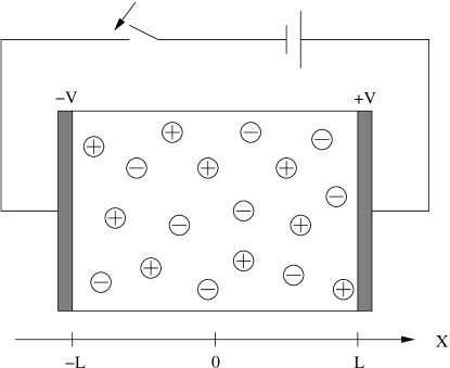
Figure 1: Sketch of the model problem (from Ref. Bazant et al. (2004)). A voltage $2V$ is suddenly applied to a dilute, symmetric, binary electrolyte between parallel-plate, blocking electrodes separated by $2L$.

First off, we note that, in this simple geometry, the gradients are replaced by $\frac{\partial}{\partial x}$ and the derivative with respect to surface normal is replaced by $\frac{\partial}{\partial x}$ at $x=-L,$ and by $-\frac{\partial}{\partial x}$ at $x=L.$ Following Bazant et al. (2004), we cast the MPNP equations in dimensionless form using $L$ as the reference length scale, and $\tau_{c}=\lambda_{D}L/D$ as the reference time scale, thus time and space are represented by $t=\tau D/\lambda_{D}L$ and $\tilde{x}=x/L.$ The problem is better formulated through the reduced variables $c=\frac{1}{2c_{0}}\left(c_{+}+c_{-}\right)$ for the local salt concentration, $\rho=\frac{1}{2c_{0}}\left(c_{+}-c_{-}\right)$ for the local charge density, and $\phi=ze\psi/kT$ for the electrostatic potential. The solution is determined by three dimensionless parameters: $\upsilon=zeV/kT,$ the ratio of the applied voltage to thermal voltage, $\epsilon=\lambda_{D}/L,$ the ratio of the Debye length to the system size, $\delta=\lambda_{S}/\lambda_{D}$ introduced in section II which measures the surface capacitance, and finally a new parameter quantifying the role of steric effects $\nu=2a^{3}c_{0},$ the effective volume fraction of the ions at no applied voltage. After dropping the tildes from the variable $x$, the dimensionless equations take the form

$$\frac{\partial c}{\partial t} =\epsilon\frac{\partial}{\partial x}\left(\frac{\partial c}{\partial x}+\rho\frac{\partial\phi}{\partial x}+\frac{\nu c}{1-\nu c}\frac{\partial c}{\partial x}\right)$$

$$\frac{\partial\rho}{\partial t} =\epsilon\frac{\partial}{\partial x}\left(\frac{\partial\rho}{\partial x}+c\frac{\partial\phi}{\partial x}+\frac{\nu\rho}{1-\nu c}\frac{\partial c}{\partial x}\right)$$

$$-\epsilon^{2}\frac{\partial^{2}\phi}{\partial x^{2}}=\rho$$ (17)

with completely blocking boundary conditions at $x=\pm 1,$

$$\frac{\partial c}{\partial x}+\rho\frac{\partial\phi}{\partial x}+\nu\frac{c}{1-\nu c}\frac{\partial c}{\partial x} =0$$ (18)

$$\frac{\partial\rho}{\partial x}+c\frac{\partial\phi}{\partial x}+\nu\frac{\rho}{1-\nu c}\frac{\partial c}{\partial x} =0$$

in addition to (16), which reads

$$\phi\pm\delta\epsilon\frac{\partial\phi}{\partial x}=\pm\upsilon$$ (19)

at $x=\pm 1$, where again $\delta$ measures the effective thickness of the surface insulating layer. Because it is impossible to satisfy all the boundary conditions when $\epsilon=0$, the limit of vanishing screening length, $\epsilon\rightarrow 0,$ is singular. The total diffuse charge near the cathode, scaled by $2zec_{0}L$, is

$$q(t)=\int_{-1}^{0}\rho(x,t)dx$$ (20)

The dimensionless Faradaic current, scaled to $2zec_{0}D/L$, is

$$j_{F}=\frac{\partial\rho}{\partial x}+c\frac{\partial\phi}{\partial x}+\nu\frac{\rho}{1-\nu c}\frac{\partial c}{\partial x}.$$ (21)

We have numerically solved these equations for various values of the dimensionless parameters. As a complete description of this large parameter space would be very lengthy, we focus on a few situations for which we provide plots meant to illustrate the differences brought in by accounting for steric effects. We therefore also plot the outcome of classical PNP in the same situations (which correspond to $\nu=0$ in the equations). Of course a systematic difference is that with the MPNP neither the concentration $c$ nor the charge density $\rho$ ever overcome the steric limit $1/\nu$.

For sake of readability of the figure, we start in Fig.2 with untypically large values for both the $\epsilon=0.1$ and $\nu=0.25$. The potential is ten times larger than the thermal voltage $\upsilon=10$. The map of the concentration and charge density are given for different instants after the application of the potential drop. Build-up of the double layers, and the consequent depletion of salt in the bulk are visible. The MPNP solution stays bounded by $1/\nu$ as promised, whereas the PNP solution blows up exponentially. A consequent observation is that salt depletion in the bulk is weaker with the MPNP, whereas with the classical PNP bulk concentrations drop to small values even for this moderate potential ($\sim 0.25~{}V$ in dimensional units). Of course, this is also a consequence of the large $\epsilon.$

For a simulation with more realistic values, we have taken $\upsilon=40$ (corresponding to $1~{}V$ in dimensional units), and $\epsilon=\nu=0.01.$ The corresponding solutions are plotted at nondimensional times $t=0,0.5,1,2,4,6,8,10,...,50$ in Fig.3. Figure 3(a) shows the bulk concentration dynamics, whereas Figure 3(b) focuses on the double layer near the boundary at $x=-1.$ The MPNP solution again stays bounded by $1/\nu=100$. The PNP solution is not plotted as it blows up in the double layer to about $\cosh(40)\approx 10^{17}$ times the bulk value (itself consequently very small), requiring subtle numerical methods. With the MPNP, the charge build up of the double layer first proceeds as it would with the PNP until concentrations close to the threshold $1/\nu$ are reached. Thereafter, charging proceeds by growth of the double layer thickness at almost constant density.

(a)

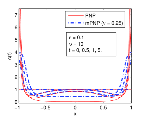
(b)

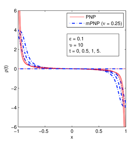
Figure 2: The numerical solutions to the PNP and MPNP systems. The dimensionless charging voltage is $\upsilon=10$, which corresponds to approximately 0.25 Volts at room temperature. The very large values of $\epsilon=0.1$ and $\nu=0.25$ are chosen deliberately for illustration. The dimensionless bulk concentration field $c$ is shown in (a), and the dimensionless charge density $\rho$ in (b)

(a)

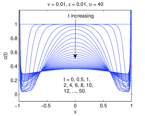
(b)

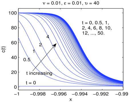
Figure 3: The numerical solution to the MPNP system at the dimensionless times (i.e. time scaled to the charging time) $t=0,0.5,1,2,4,6,8,10,...,50.$ The dimensionless charging voltage is $\upsilon=40$, which corresponds to approximately 1 Volt at room temperature. The parameters $\epsilon=\nu=0.01$ are still large, but comparatively realistic. The dimensionless bulk concentration field $c$ is shown (a) globally for the whole region (b) zoomed in at the double layer.

IV Asymptotic Analysis

In this section, we adapt to the MPNP equations introduced here the asymptotic analysis presented in Bazant et al. (2004) for PNP equations in the limit of thin double layers. We show rigourously that the key properties of the charging dynamics remain the same, namely, at leading order the boundary layer acts like a capacitor with a total surface charge density $\tilde{q}(t)$ that changes in response to the Ohmic current density $\bar{j}(t)$ from the bulk. However, the expressions for the capacitance of the double layer, and the diffusive flux from the bulk into the double layer do change, as we already discussed in Part I.

IV.1 Inner and Outer Expansions

Adopting the notation in Bazant et al. (2004), we seek regular asymptotic expansions in $\epsilon$. We observe that the system has the following symmetries about the origin

$$c(-x,t)=c(x,t),\text{ }\rho(-x,t)=-\rho(x,t),\text{ }\phi(-x,t)=-\phi(x,t)$$

therefore, we consider only $-1<x<0.$

The outer solution, in the bulk, is denoted by a bar accent, and the expansion takes the form

$$c=\bar{c}(x,t)=\bar{c}_{0}+\epsilon\bar{c}_{1}+...$$

It is easy to check that $\bar{c}_{0}=1,$ $\bar{\rho}_{0}=0$ and $\bar{\phi}_{0}=\bar{j}(t)x$ as a direct consequence of our choice for the time scale as $\tau_{c}.$ As to the inner solutions (i.e.$x\approx-1)$, we remove the singularity of equation $(\ref{potential})$ by introducing $\xi=(1+x)/\epsilon.$ Then, we obtain

$$\epsilon\frac{\partial c}{\partial t} =\frac{\partial}{\partial\xi}\left(\frac{\partial c}{\partial\xi}+\rho\frac{\partial\phi}{\partial\xi}+\frac{\nu c}{1-\nu c}\frac{\partial c}{\partial\xi}\right)$$ (22)

$$\epsilon\frac{\partial\rho}{\partial t} =\frac{\partial}{\partial\xi}\left(\frac{\partial\rho}{\partial\xi}+c\frac{\partial\phi}{\partial\xi}+\frac{\nu\rho}{1-\nu c}\frac{\partial c}{\partial\xi}\right)$$ (23)

$$-\frac{\partial^{2}\phi}{\partial\xi^{2}} =\rho$$ (24)

for which, we can seek regular asymptotic expansions

$$c=\tilde{c}(\xi,t)=\tilde{c}_{0}+\epsilon\tilde{c}_{1}+...$$

Matching inner and outer solutions in space involves the usual van Dyke conditions, e.g.

$$\lim_{\xi\rightarrow\infty}\tilde{c}(\xi,t)=\lim_{x\rightarrow-1}\bar{c}(x,t)$$

which implies $\tilde{c}_{0}(\infty,t)=\bar{c}_{0}(-1,t),$ $\tilde{c}_{1}(\infty,t)=\bar{c}_{1}(-1,t),$ etc. As seen from equations (22)-(24), there are no terms with time derivatives at leading order. This quasiequilibrium occurs, because the charging time $\tau_{c}$ is much larger than the Debye time $\tau_{D}=\lambda_{D}^{2}/D,$ which is the characteristic time scale for the local dynamics in the boundary layer. Consequently, the leading order solution is the ”equilibrium”

$$\tilde{c}_{0}=\frac{\cosh\tilde{\Phi}_{0}}{1+\nu\left(\cosh\tilde{\Phi}_{0}-1\right)},\text{ }\tilde{\rho}_{0}=\frac{-\sinh\tilde{\Phi}_{0}}{1+\nu(\cosh\tilde{\Phi}_{0}-1)}$$

where the excess voltage relative to the bulk

$$\tilde{\Phi}=\tilde{\phi}(\xi,t)-\bar{\phi}(-1,t)\sim\tilde{\Phi}_{0}+\epsilon\tilde{\Phi}_{1}+...$$

satisfies the modified PB equation at leading order

$$\frac{\partial^{2}\tilde{\Phi}_{0}}{\partial\xi^{2}}=\frac{\sinh\tilde{\Phi}_{0}}{1+\nu\left(\cosh\tilde{\Phi}_{0}-1\right)}$$ (25)

with $\tilde{\Phi}_{0}(\infty,t)=0,$ and $\tilde{\Phi}_{0}(0,t)=\tilde{\zeta}(t),$ the dimensionless zeta potential, which varies as the diffuse layer charges. Applying matching to the electric field, we obtain

$$\frac{\partial\tilde{\phi}}{\partial\xi}\left(\infty,t\right)\sim\epsilon\frac{\partial\bar{\phi}}{\partial x}(-1,t)\text{ }\Rightarrow\text{ }\frac{\partial\tilde{\phi}_{0}}{\partial\xi}(\infty,t)=0$$ (26)

and therefore an integration of (25) yields

$$\frac{\partial\tilde{\Phi}_{0}}{\partial\xi}=-\mbox{sign}(\tilde{\Phi}_{0})\sqrt{\frac{2}{\nu}\ln\left(1+\nu\left(\cosh\tilde{\Phi}_{0}-1\right)\right)}$$ (27)

IV.2 Time-dependent matching

So far we have found that both the bulk and the boundary layers are in quasiequilibrium, which apparently contradicts the dynamic nature of the charging process. This is reconciled by noting once more that the boundary condition for the inner solution involves the quantity $\zeta(t),$ which varies in response to the diffusive flux from the bulk. Motivated by the physics, we consider the total diffuse charge, which has the scaling $q(t)\sim\epsilon\tilde{q}(t),$ where

$$\tilde{q}(t)=\int_{0}^{\infty}\tilde{\rho}(\xi,t)d\xi\sim\tilde{q}_{0}+\epsilon\tilde{q}_{1}+\epsilon^{2}\tilde{q}_{2}+...$$ (28)

Taking a time derivative, and using (23) together with the no flux boundary condition (18), we obtain

$$\frac{d\tilde{q}}{dt}(t) =\lim_{\xi\rightarrow\infty}\frac{1}{\epsilon}\left(\frac{\partial\tilde{\rho}}{\partial\xi}+\tilde{c}\frac{\partial\phi}{\partial\xi}+\frac{\nu\tilde{\rho}}{1-\nu\tilde{c}}\frac{\partial\tilde{c}}{\partial\xi}\right)$$

$$\sim\lim_{x\rightarrow-1}\left(\frac{\partial\bar{\rho}}{\partial x}+\bar{c}\frac{\partial\phi}{\partial x}+\frac{\nu\bar{\rho}}{1-\nu\bar{c}}\frac{\partial\bar{c}}{\partial x}\right)$$

where we applied matching to the flux densities. Substituting the regular expansions of inner and outer solutions yield a hiararchy of matching conditions. At leading order, we have

$$\frac{d\tilde{q}_{0}}{dt}(t)=\bar{j}_{0}(t)$$ (29)

which, being a balance of $O(1)$ quantities, is reassuring us that we have chosen the correct time-scale. This is the key equation which tells us that at leading order, the double layer behaves like a capacitor, whose total surface charge density $\tilde{q},$ changes in response to the transient Faradaic current density, $\bar{j}(t),$ from the bulk.

IV.3 Leading Order Dynamics

Using equations (24),(26) and (27), the integral in (28) can be performed at leading order to yield

$$\tilde{q}_{0}(t)=-\mbox{sign}(\tilde{\zeta}_{0})\sqrt{\frac{2}{\nu}\ln[1+\nu(\cosh\tilde{\zeta}_{0}-1)]}$$ (30)

Then the Stern boundary condition, eq.(19), yields

$$\tilde{\zeta}_{0}+\delta\mbox{sign}(\tilde{\zeta}_{0})\sqrt{\frac{2}{\nu}\ln[1+\nu(\cosh\tilde{\zeta}_{0}-1)]}$$

$$=\bar{j}_{0}(t)-\upsilon=\tilde{\Psi}_{0}$$ (31)

where $\tilde{\Psi}(t)=-\upsilon-\bar{\phi}(-1,t)\sim\tilde{\Psi}_{0}+\epsilon\tilde{\Psi}_{1}+...$ is the total voltage across the compact and the diffuse layers. Equation (31) results in higher $\tilde{\zeta}_{0}$ than its classical PNP (or PB) counterpart

$$\tilde{\zeta}_{0}+2\delta\sinh(\tilde{\zeta}_{0}/2)=\tilde{\Psi}_{0}$$ (32)

because the left hand side of (31) is always smaller than the left hand side of (32) for any given $\tilde{\zeta}_{0}.$ In both formulas, the first term (i.e. $\tilde{\zeta}_{0}$) is the voltage drop over the diffuse layer whereas the second term (i.e. $-\delta\tilde{q}_{0})$ is the voltage drop over the Stern layer. For high applied voltages, the standard model assigns exponentially bigger proportions of that voltage to the Stern layer, whereas the modified theory predicts a balanced distribution. For more details, see Part I section V.

Substituting into the matching condition (29), we obtain an ordinary initial value problem

$$-\tilde{C}_{0}(\tilde{\Psi}_{0})\frac{d\tilde{\Psi}_{0}}{dt}=\tilde{\Psi}_{0}+\upsilon,\text{ }\bar{j}_{0}(0)=\upsilon$$ (33)

where

$$\tilde{C}_{0} =-\frac{d\tilde{q}_{0}}{d\tilde{\Psi}_{0}}$$ (34)

$$=\frac{1}{\frac{1+\nu(\cosh\tilde{\zeta}_{0}-1)}{|\sinh\tilde{\zeta}_{0}|}\sqrt{\frac{2}{\nu}\ln(1+\nu(\cosh\tilde{\zeta}_{0}-1))}+\delta}$$

is the differential capacitance for the double layer as a function of its voltage. This has a completely different behaviour than its counterpart in Bazant et al. (2004), namely

$$\tilde{C}_{0}=\frac{1}{\mbox{sech}(\tilde{\zeta}_{0}/2)+\delta}$$ (35)

especially at higher $\tilde{\zeta}_{0}.$ As $\tilde{\zeta}_{0}\rightarrow\infty,$ our differential capacitance $\tilde{C}_{0}^{\nu}\sim(\sqrt{\frac{2}{\nu}\tilde{\zeta}_{0}}+\delta)^{-1}\rightarrow 0,$ in contrast to $\tilde{C}_{0}^{\nu=0},$ the differential capacitance given by (35), which tends to $\delta^{-1}$(see Part I for more details). Thus, at high zeta potentials, steric effects decrease the capacitance, possibly down to zero. Physically, this is because of the increasing double layer thickness as a result of excessive pile up of the ions coming from the bulk into the double layer (see Part 1).

Equation (34) is separable, and its solution can be expressed in the form

$$\tilde{\Psi}_{0}=\bar{j}_{0}(t)-\upsilon=-F^{-1}(t)$$ (36)

$$F(z)=\int_{0}^{z}\frac{\tilde{C}_{0}(u)}{\upsilon+u}du$$ (37)

Steric effects reduce the capacitance, and therefore $F(z)$, which by formula (37) implies a faster relaxation process for the voltage difference $\tilde{\Psi}_{0}$. In other words, the $RC$ relaxation time is shortened (see Part I).

IV.4 Neutral Salt Adsorption by the Double Layer

A natural consequence of reduced capacitance at the electrodes is the reduction of the amplitude of the diffusion layer in the bulk were the adsorbed salt in the double layer is extracted from. We now revisit some of the ideas in Bazant et al. (2004), and recalculate the neutral salt adsorption by the double layer. The excess ion concentration, $c-c_{0},$ acquired by the double layers is accounted for by the diffusion from the bulk at $O(\epsilon)$ or higher, as diffusion is absent at leading order. Following Bazant et al. (2004), we introduce the variable $w(t)=\epsilon\tilde{w}(t),$ akin to $q(t),$ which represents the excess amount of salt in the double layer:

$$\tilde{w}(t)=\int_{0}^{\infty}\left[\tilde{c}(\xi,t)-\bar{c}_{0}(-1,t)\right]d\xi=\tilde{w}_{0}(t)+\epsilon\tilde{w}_{1}(t)+...$$

Taking a time derivative, we find

$$\frac{d\tilde{w}_{0}}{dt}(t) =\lim_{\xi\rightarrow\infty}\frac{1}{\epsilon}\left(\frac{\partial\tilde{c}}{\partial\xi}+\tilde{\rho}\frac{\partial\phi}{\partial\xi}+\frac{\nu\tilde{c}}{1-\nu\tilde{c}}\frac{\partial\tilde{c}}{\partial\xi}\right)$$

$$\sim\lim_{x\rightarrow-1}\left(\frac{\partial\bar{c}}{\partial x}+\bar{\rho}\frac{\partial\phi}{\partial x}+\frac{\nu\bar{c}}{1-\nu\bar{c}}\frac{\partial\bar{c}}{\partial x}\right)$$ (38)

Since $\bar{c}=1+\epsilon\bar{c}_{1}+...$ , at leading order $\bar{c}\sim 1$ and $\frac{\partial\bar{c}}{\partial}\sim\epsilon\frac{\partial\bar{c}_{1}}{\partial x},$ therefore (38) yields

$$\frac{d\tilde{w}_{0}}{d\bar{t}}(t)=\frac{\left(1-\nu\right)}{\epsilon}\frac{d\tilde{w}_{0}}{dt}(t)=\frac{\partial\bar{c}_{1}}{\partial x}(-1,t)$$ (39)

which involves the new time variable

$$\bar{t}=\frac{\epsilon}{\left(1-\nu\right)}t=\frac{\epsilon}{\left(1-\nu\right)}\frac{\tau}{\tau_{c}}=\frac{\tau}{\tau_{s}}$$

scaled to bulk diffusion time, $\tau_{s}=\left(1-\nu\right)L^{2}/D,$ which is slightly different from the time scale given in Bazant et al. (2004). The salt uptake $\tilde{w}(t)$ can be expressed in terms of an integral

$$\tilde{w}(t) =\int_{0}^{\infty}\left(\frac{\cosh\tilde{\Phi}}{1+\nu\left(\cosh\tilde{\Phi}-1\right)}-1\right)d\xi$$

$$=\int_{0}^{\zeta}\frac{\cosh\tilde{\Phi}-1}{1+\nu\left(\cosh\tilde{\Phi}-1\right)}\frac{\left(1-\nu\right)d\tilde{\Phi}}{\sqrt{\frac{2}{\nu}\ln\left(1+\nu\left(\cosh\tilde{\Phi}-1\right)\right)}}$$ (40)

with no obvious further simplification.

We now proceed to calculate the depletion of the bulk concentration during the double-layer charging. Note that the new time scale $\tau_{s}$ introduced by (39) is the time scale for the first order diffusive dynamics in bulk

$$\frac{\partial\bar{c}_{1}}{\partial\bar{t}}=\frac{\left(1-\nu\right)}{\epsilon}\frac{\partial\bar{c}_{1}}{\partial t}=\frac{\partial^{2}\bar{c}_{1}}{\partial x^{2}}$$ (41)

As the source is defined by (39) in terms of gradients, an appropriate Green’s function can be obtained by taking Laplace transforms and using method of images as in Bazant et al. (2004), which leads to

$$\bar{c}_{1}(x,t)=-\int_{0}^{\bar{t}}d\bar{t}^{\prime}G(x,\bar{t}-\bar{t}^{\prime})\frac{\partial}{\partial\bar{t}}[\tilde{w}_{0}(\bar{t}^{\prime}/\epsilon)]$$ (42)

where

$$G(x,\bar{t})=\frac{1}{\sqrt{\pi\bar{t}}}\sum_{m=-\infty}^{\infty}e^{-\left(x-2m+1\right)^{2}/4\bar{t}}$$ (43)

In the limit $\epsilon\rightarrow 0,$ the initial charging process at the time scale $\tau_{c}=O\left(\epsilon\right)$ is almost instantaneous, which is followed by the slow relaxation of the bulk diffusion layers. This limit corresponds to approximating the source terms in the integral in (42) to exist only in a small $O\left(\epsilon\right)$ neighborhood of zero, or more explicitly

$$\lim_{\epsilon\rightarrow 0}\bar{c}_{1}(x,\bar{t}) \simeq-G(x,\bar{t})\int_{0}^{\bar{t}}d\bar{t}^{\prime}\frac{\partial}{\partial\bar{t}}[\tilde{w}_{0}\left(\frac{\bar{t}^{\prime}}{\epsilon}\right)]$$

$$=-\tilde{w}_{0}\left(\infty\right)G(x,\bar{t})$$ (44)

with $\tilde{w}_{0}\left(\infty\right)=$

$$\int_{0}^{f^{-1}(\upsilon)}\frac{\cosh\tilde{\Phi}-1}{1+\nu\left(\cosh\tilde{\Phi}-1\right)}\frac{\left(1-\nu\right)d\tilde{\Phi}}{\sqrt{\frac{2}{\nu}\ln\left(1+\nu\left(\cosh\tilde{\Phi}-1\right)\right)}}$$ (45)

where

$$f(\zeta)=\zeta+\mbox{sign}(\zeta)\delta\sqrt{\frac{2}{\nu}\ln\left(1+\nu\left(\cosh\zeta-1\right)\right)}.$$ (46)

As expected from the underlying physics, and already explained in Part I and illustrated in the plots of section III above, the formula (45) predicts smaller values for the the depth of the bulk diffusion than its classical PNP ($\nu=0)$ counterpart. This difference is more pronounced at higher $\upsilon.$ Equation (44) is a simple approximation that describes two diffusion layers created at the electodes slowly invading the entire cell. At first,they have simple Gaussian profiles

$$\bar{c}(x,t)\sim 1-\frac{\epsilon\tilde{w}_{0}\left(\infty\right)}{\sqrt{\pi\bar{t}}}\left[e^{-\left(x+1\right)^{2}/4\bar{t}}+e^{-\left(x-1\right)^{2}/4\bar{t}}\right]$$ (47)

for $\epsilon<<\bar{t}<<1.$ The two diffusion layers eventually collide, and the concentration slowly approaches a reduced constant value,

$$\bar{c}(x,t)\sim 1-\epsilon\tilde{w}_{0}\left(\infty\right)$$ (48)

for $\bar{t}>>1,$ as we expect from the steady-state excess concentration from the double layers.

Of course one expects that at large enough applied voltage, the above approximation breaks down, as the decrease in bulk concentration becomes significant and thus modifies the value of $w$ in the double layer.

IV.5 Validity of the Weakly Nonlinear Approximation

The first order solution consisting of the variables indexed by ”0” is often referred to as the weakly nonlinear approximation, whose main feature is that the bulk concentrations are constant, namely $\bar{c}\approx\bar{c}_{0}=1$ and $\bar{\rho}\approx\bar{\rho}_{0}=0.$ The system therefore is characterized only by the surface charge $\tilde{q}\approx\tilde{q}_{0},$ or the double layer potential difference $\tilde{\Psi}\approx\tilde{\Psi}_{0},$ which is governed by the nonlinear ODE in equation (33). This corresponds to modeling the problem by an equivalent circuit model with variable capacitance for the double layer, and constant bulk electrolyte resistance.

In order to understand when the weakly nonlinear approximation holds, we can compare the size of the next order approximation to the leading term. Although not a rigorous proof, one may argue that if $|\epsilon c_{1}|$ is much smaller than $\bar{c}_{0}=1,$ then leading order term is a good approximation to the full solution. We will get help from the approximations (47) and (48) to see if this is the case.

Seen in the light of equation (48), the assumption that the first correction is much smaller than the leading term requires that $\nu_{b}=\epsilon\tilde{w}_{0}\left(\infty\right)\ll 1,$ in other words $\epsilon\left(1-\nu\right)\int_{0}^{f^{-1}(\upsilon)}\frac{\cosh\Phi-1}{1+\nu\left(\cosh\Phi-1\right)}\frac{d\Phi}{\sqrt{\frac{2}{\nu}\ln\left(1+\nu\left(\cosh\Phi-1\right)\right)}}\ll 1,$ where $f$ is given in (46). After a series of approximations, including $\left(1-\nu\right)\approx 1,$ $\delta=O(1),$ and $\zeta\gg 1$(or $\upsilon\gg 1),$ this becomes $\epsilon\sqrt{\frac{2}{\nu}\ln\left(1+\nu\cosh\upsilon\right)}\ll 1.$ If $\nu$ is not too close to zero(i.e. $\nu\cosh\upsilon\gg 1)$, this is the same as $2\epsilon^{2}\upsilon/\nu\ll 1.$ Putting the units back, we obtain

$$2\frac{\lambda_{D}^{2}}{L^{2}a^{3}c_{0}}\frac{zeV}{kT}\ll 1$$ (49)

For a typical experiment with $\lambda_{D}=10$ nm, $L=0.1mm,$ $c_{0}=1mM,$ $a=5\mathring{A},$ and at room temperature, this condition becomes $V\ll 188$ Volts.

However, the weakly nonlinear dynamics breaks down at somewhat smaller voltages, because the neutral salt adsorption causes a temporary, local depletion of bulk concentration exceeding that of the final steady state. In our model problem, the maximum change in bulk concentration occurs just outside the diffuse layers at $x=\pm 1,$ just after the initial charging process finishes at the same scale $t=O(1)$ or $\bar{t}=O(\epsilon).$ Letting $\bar{t}=\epsilon,$ and $x=\pm 1$ in equation (47), we obtain the first two terms in the asymptotic expansion as

$$c\left(\pm 1,\epsilon\right)=1-\sqrt{\frac{\epsilon}{\pi}}\tilde{w}_{0}\left(\infty\right)$$

At that time, the double layers have almost been fully charged , however the bulk diffusion has only had time to reach a region of length $O\left(\sqrt{\epsilon}\right).$So the concentration is depleted locally by $O\left(\frac{\epsilon}{\sqrt{\epsilon}}\right)=O\left(\sqrt{\epsilon}\right),$ which is much more than the uniform $O(\epsilon)$ depletion remaining after complete bulk diffusion.

Therefore, in order for the time-dependent correction term to be uniformly smaller than the leading term, we need

$$\sqrt{\frac{\epsilon}{\pi}}\tilde{w}_{0}\left(\infty\right)\ll 1$$ (50)

By the same approximations as in (49), this yields $\frac{2\epsilon\upsilon}{\sqrt{\pi}\nu}\ll 1,$ or with the units

$$\frac{2}{\sqrt{\pi}}\frac{\lambda_{D}}{La^{3}c_{0}}\frac{zeV}{kT}\ll 1$$ (51)

The corresponding threshold voltage is smaller than the former by a factor of roughly $\sim L/\lambda_{D}=\epsilon^{-1}$. For the same set of parameter as above $\lambda_{D}=10$ nm, $L=0.1mm,$ $c_{0}=1mM,$ $a=5\mathring{A},$ and at room temperature, this condition gives $V\ll 0.033$ Volts. Thus according to this criterion, the weakly nonlinear approximation easily breaks down, and one may need to consult to the full MPNP system for an understanding of the electrolyte dynamics.

A more accurate understanding into the condition (50) is gained by the numerical study of the function $w.$ The curves on which $\sqrt{\epsilon}w=1$ (i.e. $\epsilon=w^{-2}$) are plotted in Fig.4 for various values of $\nu$ (here we dropped the somewhat arbitrary factor $\sqrt{\pi}$ in (50)).The weakly nonlinear approximation holds to the south-west of these curves when $\sqrt{\epsilon}w\ll 1.$ The criterion given by the inequality (51) corresponds to the asymptotic behaviour of those curves as $\upsilon$ tends to infinity.

To observe that this is the case numerically, we have also compared the charging dynamics given by the weakly nonlinear approximation to that of the full MPNP solution in Fig.5. with the parameters $\epsilon=\nu=0.01.$ When the parameters were to the south-west of the $\sqrt{\epsilon}w=1,$ as in case (c), the match was perfect. In the other cases, the weakly nonlinear approximation did not do as well, it was particularly off for case (b), when the product $\sqrt{\epsilon}w$ yielded the highest number. In case (a), the agreement was off by a constant shift, whereas in case (d), the situation improved over time. This is because $\epsilon w$ is still small for case (d), although $\sqrt{\epsilon}w$ is not, and therefore weakly nonlinear approximation is still valid for the final state of the system. To summarize, if an accurate description of the system at all times is desired, then $\sqrt{\epsilon}w<<1$ is the appropriate criterion, however it may suffice to have just $\epsilon w<<1$ to be able to predict the eventual steady state by the weakly nonlinear model.

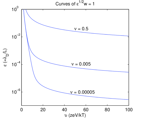
Figure 4: Shown are the curves on which $\sqrt{\epsilon}w=1$ for various values of $\nu.$ The weakly nonlinear approximation holds to the south-west of these curves when $\sqrt{\epsilon}w<<1.$

(I)

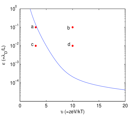
(II)

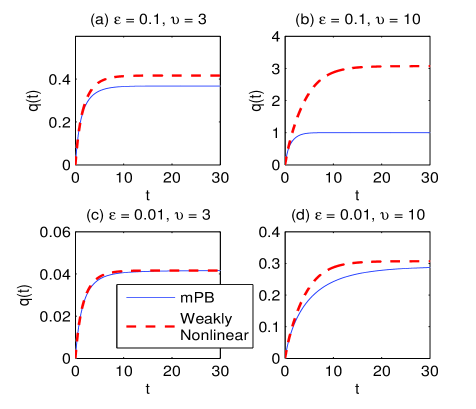
Figure 5: Four case studies on the validity of the weakly nonlinear approximation. No stern capacitance is included ($\delta=0$). (I) The $\sqrt{\epsilon}w=1$ curve for the particular value $\nu=0.01,$ and corresponding locations of the four case studies shown. (II) The comparison of the charge $q(t)$ stored in the half cell computed by (i) the MPNP (ii) the weakly nonlinear approximation corresponding to the MPNP. The match in (c) is good as expected, and the match in (b) is off by several factors, again as expected. In cases (a) and (d), the curves run close but they are clearly separated.

V Conclusions

As an extension of the modified PB approach, we have derived modified PNP equations, which may be of help when the thin double layer approximation fails. Using this new set of equations, we have revisited the model problem of the step charging of a cell with parallel blocking electrodes. In addition, we have confirmed through asymptotic analysis the hypotheses stated in Part I regarding the MPB double layer model. We have also investigated the limits of the thin double layer approximation as well as higher order corrections.

The MPNP system proposed is a natural extension of one of the two models introduced in Part I, namely the MPB model based on an approach originally due to Iglic and Kralj-Iglic (1994); Borukhov et al. (1997). One can similarly construct other MPNP equations from other MPB models such as the composite diffuse-layer model also introduced in Part I. However the discontinuous structure of the latter leads to a complex formalism with discontinuities, improper for implementation in complex geometries, whereas the one presented here has a smooth behavior and is therefore much more broadly applicable.

We expect that the MPNP equations presented here, or other simple variations with different modifications of the chemical potentials or free energy, will find many applications. They are no more difficult to use than the classical PNP equations, which are currently ubiquitous in the modeling of electrochemical systems. Especially at large voltages, the MPNP equations are much better suited for numerical computations, since they lack the exponentially diverging concentrations predicted by the PNP equations, which are difficult to resolve. Of course, those same divergences are also clearly unphysical, while the MPNP equations predict reasonable ion profile for any applied voltage.

Future research directions include the application of the presented framework to many other settings including the response of the simple electrolytic cell considered here to various systems with time-dependent applied voltages of strong amplitudes. In particular, driving an electrochemical cell or AC electro-osmotic pump at rather large frequencies should be a selective way of checking the validity/use of equations such as the one put forward here because dynamical effects are exacerbated in such situations.

References

- Bazant et al. (2004) M. Z. Bazant, K. Thornton, and A. Ajdari, Phys. Rev. E 70, 021506 (2004).
- Lyklema (1995) J. Lyklema, Fundamentals of Interface and Colloid Science. Volume II: Solid-Liquid Interfaces (Academic Press Limited, San Diego, CA, 1995).
- Ramos et al. (1999) A. Ramos, H. Morgan, N. G. Green, and A. Castellanos, J. Colloid Interface Sci. 217, 420 (1999).
- Brown et al. (2001) A. B. D. Brown, C. G. Smith, and A. R. Rennie, Phys. Rev. E 63, 016305 (2001).
- Studer et al. (2004) V. Studer, A. Pépin, Y. Chen, and A. Ajdari, Analyst 129, 944 (2004).
- Levitan et al. (2005) J. A. Levitan, S. Devasenathipathy, V. Studer, Y. Ben, T. Thorsen, T. M. Squires, and M. Z. Bazant, Colloids and Surfaces A 267, 122 (2005).
- Urbanski et al. (2006) J. P. Urbanski, J. A. Levitan, M. Z. Bazant, and T. Thorsen, Applied Physics Letters (2006), submitted.
- Macdonald (1990) J. R. Macdonald, Electrochim. Acta 35, 1483 (1990).
- Geddes (1997) L. A. Geddes, Ann. Biomedical Eng. 25, 1 (1997).
- Newman (1991) J. Newman, Electrochemical Systems (Prentice-Hall, Inc., Englewood Cliffs, NJ, 1991), 2nd ed.
- Bard and Faulkner (2001) A. J. Bard and L. R. Faulkner, Electrochemical Methods (John Wiley & Sons, Inc., New York, NY, 2001).
- Newman (1965) J. Newman, Trans. Faraday Soc. 61, 2229 (1965).
- Rubinstein and Zaltzman (2000) I. Rubinstein and B. Zaltzman, Phys. Rev. E 62, 2238 (2000).
- Eisenberg (1999) R. Eisenberg, J. Mem. Bio. 171, 1 (1999).
- M.G. Kumikova and Nitzan (1999) P. G. M.G. Kumikova, R.D. Coalson and A. Nitzan, Biophys. 76, 642 (1999).
- A.E. Cardenas and Kurnikova (2000) R. C. A.E. Cardenas and M. Kurnikova, Biophys. 79, 80 (2000).
- U. Hollerbach and Eisenberg (2000) D. B. U. Hollerbach, D.P. Chen and B. Eisenberg, Langmuir 16, 5509 (2000).
- U. Hollerbach (2002) R. E. U. Hollerbach, Langmuir 18, 3626 (2002).
- Ajdari (2000) A. Ajdari, Phys. Rev. E 61, R45 (2000).
- González et al. (2000) A. González, A. Ramos, N. G. Green, A. Castellanos, and H. Morgan, Phys. Rev. E 61, 4019 (2000).
- Ramos et al. (2003) A. Ramos, A. González, A. Castellanos, N. G. Green, and H. Morgan, Phys. Rev. E 67, 056302 (2003).
- Bazant and Ben (2006) M. Z. Bazant and Y. Ben, Lab on a Chip 6, 1455 (2006).
- Gamayunov et al. (1986) N. I. Gamayunov, V. A. Murtsovkin, and A. S. Dukhin, Colloid J. USSR 48, 197 (1986).
- Murtsovkin (1996) V. A. Murtsovkin, Colloid Journal 58, 341 (1996).
- Squires and Bazant (2004) T. M. Squires and M. Z. Bazant, J. Fluid Mech. 509, 217 (2004).
- Shilov and Simonova (1981) V. N. Shilov and T. S. Simonova, Colloid J. USSR 43, 90 (1981).
- Simonova et al. (2001) T. A. Simonova, V. N. Shilov, and O. A. Shramko, Colloid J. 63, 108 (2001).
- Squires and Bazant (2006) T. M. Squires and M. Z. Bazant, J. Fluid Mech. 560, 65 (2006).
- Bazant and Squires (2004) M. Z. Bazant and T. M. Squires, Phys. Rev. Lett. 92, 066101 (2004).
- Yariv (2005) E. Yariv, Phys. Fluids 17, 051702 (2005).
- Saintillan et al. (2006) D. Saintillan, E. Darve, and E. S. G. Shaqfeh, Journal of Fluid Mechanics 563, 223 (2006).
- Levine and Outhwaite (1977) S. Levine and C. Outhwaite, J. Chem. Soc., Faraday Trans. 2 74, 1670 (1977).
- Outhwaite and Bhuiyan (1980) C. Outhwaite and L. Bhuiyan, J. Chem. Soc., Faraday Trans. 2 76, 1388 (1980).
- S. L. Carnie and Ninham (1981) D. M. S. L. Carnie, D.Y.C. Chan and B. Ninham, J. Chem. Phys. 74, 1472 (1981).
- Outhwaite and Bhuiyan (1982) C. Outhwaite and L. Bhuiyan, J. Chem. Soc., Faraday Trans. 2 78, 775 (1982).
- Outhwaite and Bhuiyan (1983) C. Outhwaite and L. Bhuiyan, J. Chem. Soc., Faraday Trans. 2 78, 707 (1983).
- Carnie and Torrie (1984) S. L. Carnie and G. M. Torrie, Adv. Chem. Phys. 46, 141 (1984).
- Kirkwood (1934) J. Kirkwood, J. Chem. Phys. 2, 767 (1934).
- Rosenfeld (1989) Y. Rosenfeld, Phys. Rev. Lett. 63, 980 (1989).
- Rosenfeld (1994) Y. Rosenfeld, Phys. Rev. E 50, R3318 (1994).
- Rosenfeld et al. (1997) Y. Rosenfeld, M. Schmidt, H. Lowen, and P. Tarazona, Phys. Rev. E 55, 4245 (1997).
- Gillespie et al. (2002) D. Gillespie, W. Nonner, and R. S. Eisenberg, J. Phys.: Condens. Matter 14, 12129 (2002).
- Gillespie et al. (2003) D. Gillespie, W. Nonner, and R. S. Eisenberg, Phys. Rev. E 68, 031503 (2003).
- Gillespie et al. (2005) D. Gillespie, M. Valisko, and D. Boda, J. Phys.: Condens. Matter 17, 6609 (2005).
- Roth and Gillespie (2005) R. Roth and D. Gillespie, Phys. Rev. Lett. 95, 247801 (2005).
- Wicke and Eigen (1952) E. Wicke and M. Eigen, Z. Elektrochem. 56, 551 (1952).
- Freise (1952) V. Freise, Z. Elektrochem. 56, 822 (1952).
- Eigen and Wicke (1954) M. Eigen and E. Wicke, J. Phys. Chem. 58, 702 (1954).
- Iglic and Kralj-Iglic (1994) A. Iglic and V. Kralj-Iglic, Electrotecnical Rev. (Slovenia) 61, 127 (1994).
- Kralj-Iglic and Iglic (1996) V. Kralj-Iglic and A. Iglic, J. Phys. II France 6, 477 (1996).
- Bohinc et al. (2001) K. Bohinc, V. Kralj-Iglic, and A. Iglic, Electrochim. Acta 46, 3033 (2001).
- Bohinc et al. (2002) K. Bohinc, A. Iglic, T. Slivnik, and V. Kralj-Iglic, Bioelectrochemistry 57, 73 (2002).
- Borukhov et al. (1997) I. Borukhov, D. Andelman, and H. Orland, Phys. Rev. Lett. 79, 435 (1997).
- Borukhov et al. (2000) I. Borukhov, D. Andelman, and H. Orland, Electrochim. Acta 46, 221 (2000).
- Borukhov (2004) I. Borukhov, J. Pol. Sci. B: Pol. Phys. 42, 3598 (2004).