Stiffening of semiflexible biopolymers and cross-linked networks

Abstract

We study the mechanical stiffening behavior in two-dimensional (2D) cross-linked networks of semiflexible biopolymer filaments under simple shear. Filamental constituents immersed in a fluid undergo thermally excited bending motions. Pulling out these undulations results in an increase in the axial stiffness. We analyze this stiffening behavior of 2D semiflexible filaments in detail: we first investigate the average, static force-extension relation by considering the initially present undulated configuration that is pulled straight under a tensile force, and compare this result with the average response in which undulation dynamics is allowed during pulling, as derived earlier by MacKintosh and coworkers. We will show that the resulting mechanical behavior is rather similar, but with the axial stiffness being a factor 2 to 4 larger in the dynamic model. Furthermore, we study the stretching contribution in case of extensible filaments and show that, for 2D filaments, the mechanical response is dominated by enthalpic stretching. Based on the single-filament mechanics, we develop a 2D analytical model describing the mechanical behavior of biopolymer networks under simple shear, adopting the affine deformation assumption. These results are compared with discrete, finite-element (FE) calculations of a network consisting of semiflexible filaments. The FE calculations show that local, nonaffine filament reorientations occur that induce a transition from a bending-dominated response at small strains to a stretching-dominated response at larger strains. Stiffening in biopolymer networks thus results from a combination of stiffening in individual filaments and changes in the network topography.

I Introduction

The mechanics of eukaryotic cells is largely governed by the cytoskeleton, an interpenetrated network of biopolymer protein filaments, spanning the region between the cell’s nucleus and membrane. Its filamentous constituents are actin filaments, intermediate filaments and microtubules. It is important to gain more insight in the physical origin of the mechanical behavior of the cytoskeleton in view of its role in fundamental biological processes as cell division, cell motility and mechanotransduction. It is well known that network-like biological tissues are compliant and respond to deformation by exhibiting an increasing stiffness, i.e., the ratio of change of stress and change of strain. Experimental research on the viscoelastic strain stiffening behavior in such biopolymer networks started in the 1980’s, e.g. by means of micropipette and microtwisting experimentsWang95 and rheological experiments on in-vitro gels of cytoskeletal filaments (actin, vimentin, keratin),GardelScience04 ; Xu00 ; Tseng04 ; Janmey91 ; Ma99 neuronal intermediate filamentsLeterrier96 and fibrin.Bale88 ; Janmey83 Through these and numerous other studies, it is well-established by now that not only the filamental constituents but also the type and dynamics of cross-linking proteins govern the mechanical response of such semiflexible biopolymer networks.Wachsstock94 ; WagnerPNAS06 ; GardelPNAS06 ; DiDonnaPRL06 ; McGrath06 ; Tharmann

The mechanical behavior of semiflexible biopolymer networks has been subject to theoretical investigation since the mid nineties.MacKintoshPRL95 ; HeadPRL03 ; HeadPRE03 ; WilhelmPRL03 ; Levine ; DiDonnaPRE05 ; Storm ; HeussingerPRL06 Most studies focussed on the small-strain deformations enabling analytical treatment. The mechanics of these networks under strain is determined by the mechanical properties of individual filamental constituents, changes in network topography under deformation, and finally, the molecular properties and dynamics of cross-binding proteins. MacKintosh and co-workers developed a model to describe the elasticity of biopolymer networks, in which strain stiffening originates from longitudinal stiffening in individual semiflexible filaments.MacKintoshPRL95 Filamental stiffening is attributed to entropic effects, originating from the dynamic interactions with the surrounding (cytoplasmic) fluid.MacKintoshPRL95 ; KroyPRL96 ; Odijk ; Liu Next, Storm et al. developed a continuum model by inserting this single-filament force-extension relation in a network of infinitely many, randomly oriented filaments.Storm Under an applied shear, the network is then assumed to deform in an affine manner, allowing for an analytical description of the overall nonlinear network response.

Under the affine-deformation assumption, used in network models describing rubber elasticity,Wu93 strain stiffening of the network directly results from stiffening in individual filaments. The validity of the affinity assumption adopted by Storm et al.Storm was studied in detail by Head et al.HeadPRL03 ; HeadPRE03 and by Wilhelm and FreyWilhelmPRL03 for straight filaments. Numerical calculations in the small-strain limit show that network distortions are indeed affine for high density, highly cross-linked networks, but are nonaffine for low- and intermediate-density networks. In a recent publication we have reported on strain stiffening in two-dimensional (2D) cross-linked biopolymer networks comprising discrete filaments, analyzed by the finite-element method.OnckPRL05 With the aid of this novel approach, the network response was calculated up to large strains for various filament densities, and we showed that the origin of stiffening lies in the network rather than in its constituents. In this discrete filament model strain stiffening results from nonaffine network reorientations that induce a transition from a (relatively soft) bending-dominated response at small strains to a (stiff) stretching dominated response at large strains. Next to initially straight filaments, we studied networks of initially undulated filaments as if instantaneous thermal undulations are frozen in, and found that these merely postpone the onset of the stiffening.

Both approaches have advantages and disadvantages. The affine-network (AN) model accounts for the dynamic interaction with the surrounding fluid during pulling, but neglects any network rearrangements, while the discrete-network (DN) model accounts for the latter, but ignores the former. The aim of this article is to rigorously investigate the relative contribution of both effects on the overall stiffening by a detailed comparison of both approaches.

This article is organized as follows. In Sect. II we will determine the undulated shape of 2D semiflexible filaments resulting from the interaction with the surrounding fluid and will investigate the distribution of slack (the relative displacement of the ends to reach a straight configuration). Subsequently, in Sect. III we will study the mechanical behavior of extensible and inextensible semiflexible filaments under tension. We will in detail compare the ensemble-averaged force-extension relation of individual, inextensible filaments with and without undulation dynamics taken into account (to be referred to as the dynamic and static response, respectively) and show that the average mechanical response is rather similar. In addition, we will investigate the average static and dynamic force-extension relations in case of extensible filaments and show that the mechanical response is largely determined by the enthalpic stretching contribution, as confirmed by discrete finite-element calculations. Finally, in Sect. IV we will develop an analytical model describing the affine, mechanical behavior of 2D biopolymer networks under simple shear. As input, the model uses the average force-extension relation of individual filaments determined in Sect. III. Results will be compared with the discrete network model and we will show that nonaffine local network reorientations, that are not taken into account in the analytical model, play a key role in the onset of stiffening, especially at lower densities.

II Semiflexible filaments: shape and thermal undulations

The shape of cytoskeletal filaments such as F-actin is thermally perturbed by collisions with cytoplasmic molecules. The resistance of polymer chains to such thermal forces is characterized by their persistence length $L_{\rm P}$, the characteristic arc length above which the filaments’ tangent becomes uncorrelated. Figure 1 shows a schematic of a snapshot of a 2D thermally undulated filament of contour length $L_{\rm C}$, parameterized by the arc length $s$ and having a tangent angle $\theta(s)$.

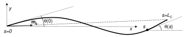
Figure 1: Schematic of a thermally undulated filament of contour length $L_{\rm C}$. The arc length along the filament is denoted by $s\in[0,L_{\rm C}]$ and its tangent relative to the $x$-axis by the angle $\theta(s)$. The unit vector along the end-to-end direction is $\mathbf{m}_{0}$.

Mathematically, the persistence length follows from the average cosine of $\theta(s)-\theta(0)$ in a filament over time or, alternatively, over all filaments in the ensemble at a specific time. For 2D filaments this average decays exponentially with arc length $s$ asHoward

$$\left<\cos[\theta(s)-\theta(0)]\right>=\exp\left[-\frac{s}{2L_{\rm P}}\right],$$ (1)

with the persistence length defined by

$$L_{\rm P}=\frac{\kappa_{\rm f}}{k_{\rm B}T}.$$ (2)

In Eq. (2), $k_{\rm B}$ is Boltzmann’s constant, $T$ is the temperature, and $\kappa_{\rm f}$ is the flexural rigidity. While biopolymers such as DNA are flexible polymers with $L_{\rm P}\ll L_{\rm C}$, we here focus on semiflexible filaments (e.g. actin, vimentin, keratin and fibrin) that have a persistence length similar to their contour length. Details on the values of $L_{\rm P}$ and $\kappa_{\rm f}$ used for the calculations in this article can be found in Appendix A.

In general, the undulated shape of filaments can be expressed by a superposition of $N$ Fourier modes for the tangent angle $\theta(s)$: Howard ; Gittes93 ; rmrkNOFT

$$\theta(s)=\sqrt{\frac{2}{L_{\rm C}}}\sum_{n=0}^{N}a_{n}^{0}\cos\left[q_{n}s\right],$$ (3)

with $q_{n}=n\pi/L_{\rm C}$. The amplitudes $a_{n}^{0}$ can be calculated for a given shape $\theta(s)$ from

$$a_{n}^{0}=\sqrt{\frac{2}{L_{\rm C}}}\int_{0}^{L_{\rm C}}\theta(s)\cos\left[q_{n}s\right]\mbox{d}s\quad\mbox{(for $n\geq 1$)}.$$

Two-dimensional, undulated filaments can thus be mimicked by using Eq. (3) in which the amplitudes $a_{n}^{0}$ are randomly chosen from a Gaussian distribution with mean value 0 and standard deviation (see Appendix B)

$$s_{n}=\sqrt{\frac{1}{L_{\rm P}}}q_{n}^{-1}\quad(n\geq 1).$$ (4)

Since $\mbox{d}x(s)=\cos\left[\theta(s)\right]\mbox{d}s$ and $\mbox{d}y(s)=\sin\left[\theta(s)\right]\mbox{d}s$, the filament’s coordinates $x(s)$ and $y(s)$ follow directly from

$$x(s)=\int_{s^{\prime}=0}^{s}\cos\left[\theta(s^{\prime})\right]\mbox{d}s^{\prime}$$ (5a)

$$y(s)=\int_{s^{\prime}=0}^{s}\sin\left[\theta(s^{\prime})\right]\mbox{d}s^{\prime}.$$ (5b)

Finally, without loss of generality, we can require the end-to-end direction to coincide with the $x$-axis, i.e., $y(0)=y(L_{\rm C})=0$. Application of the small-angle approximation in Eq. (5b), along with (3), then yields

$$0\approx\int_{0}^{L_{\rm C}}\theta(s^{\prime})\mbox{d}s^{\prime}=\sqrt{2L_{\rm C}}a_{0}^{0}\Rightarrow a_{0}^{0}\approx 0.$$ (6)

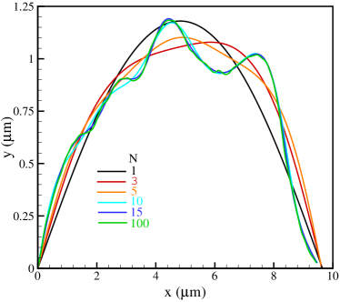
Figure 2: A semiflexible filament, randomly generated using Eqs. (3)–(6) with $L_{\rm P}=L_{\rm C}=10~{}\mu$m, for different numbers of terms, $N$, in the Fourier series.

Figure 2 shows a filament generated with the procedure described above using $L_{\rm P}=L_{\rm C}=10~{}\mu$m. The six curves all display the filament in the same configurational state, i.e., with equal (random) amplitudes $a_{n}^{0}$, but taking into account a varying number of terms $N$ in Eq. (3). As can be seen, the shape of the filament does not significantly change for $N>10$.

As a result of thermal undulations, the end-to-end distance $r_{0}$ will be smaller than the contour length $L_{\rm C}$. To estimate the mean value of $r_{0}$ we can use the mean-squared end-to-end distance given by  Howard

$$\left<r_{0}^{2}\right>=2\int_{s=0}^{L_{\rm C}}\int_{s^{\prime}=s}^{L_{\rm C}}\exp\left[-\frac{s^{\prime}-s}{2L_{\rm P}}\right]ds^{\prime}ds$$

$$=4L_{\rm P}^{2}\left(2\left\{\exp\left[-\frac{L_{\rm C}}{2L_{\rm P}}\right]-1\right\}+\frac{L_{\rm C}}{L_{\rm P}}\right)$$ (7)

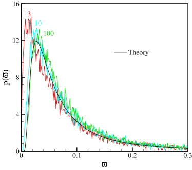
Figure 3: Probability density function $p(\varpi)$ of the relative slack $\varpi$ in semiflexible filaments with $L_{\rm P}=L_{\rm C}=10~{}\mu$m, calculated using Eq. (8) for $2\times 10^{4}$ filaments for $N=3$ (red), 10 (cyan) and 100 (green). The black, solid curve shows the theoretical distribution function, according to Eqs.(9) and (10).

For filaments as in Fig. 2 having $L_{\rm P}=L_{\rm C}=10~{}\mu$m, $\left<r_{0}\right>$ is calculated using (7) to be about $9.23~{}\mu$m. We have verified this by calculating $r_{0}=\sqrt{x^{2}(s=L_{\rm C})+y^{2}(s=L_{\rm C})}$ for $10^{5}$ filaments generated as described above with $N=10$, resulting in an avarage value of $r_{0}=9.25~{}\mu$m.remarkendpoint

The distance over which the ends of the filaments should be displaced to reach the straight configuration is $L_{\rm C}-r_{0}$, the slack distance $\xi$. The relative slack $\varpi$, defined as

$$\varpi=\frac{L_{\rm C}-r_{0}}{r_{0}},$$ (8)

has an average value of 8.1 % for these filaments. To investigate the dependence of $\varpi$ on the number of terms $N$ in the Fourier series, we plot the relative slack probability density function $p(\varpi)$ for $N=3$, 10 and 100 in Fig. 3. It can be seen that the distribution shifts to larger $\varpi$ for larger values of $N$. However, no significant difference is found between the distribution functions for $N=10$ and 100.

One can also compare the relative slack distributions with the 2D radial distribution function given by Wilhelm and FreyWilhelmPRL96 ,

$$\mathscr{G}(r_{0};L_{\rm C};L_{\rm P})=\frac{2L_{\rm P}\sqrt{L_{\rm C}}}{\sqrt{\pi}}\sum_{k\geq 0}\frac{(2k-1)!!}{2^{k}k!}\frac{1}{[2L_{\rm P}(L_{\rm C}-r_{0})]^{5/4}}\times$$

$$\exp\left[-\frac{(k+\frac{1}{4})^{2}L_{\rm C}^{2}}{2L_{\rm P}(L_{\rm C}-r_{0})}\right]D_{3/2}\left(\frac{2(k+\frac{1}{4})L_{\rm C}}{\sqrt{2L_{\rm P}(L_{\rm C}-r_{0})}}\right),~{}~{}$$ (9)

with $D_{3/2}(x)$ a parabolic cylinder function. A derivation of this equation is given in Appendix C. This function of $r_{0}=L_{\rm C}/(1+\varpi)$, normalized as $\int_{0}^{L_{\rm C}}\mathscr{G}(r_{0};L_{\rm C};L_{\rm P})\mbox{d}r_{0}=1$, can be transformed into the distribution function for the relative slack:

$$p(\varpi;L_{\rm C};L_{\rm P})=\frac{L_{\rm C}}{(1+\varpi)^{2}}\mathscr{G}\left(\frac{L_{\rm C}}{1+\varpi};L_{\rm C};L_{\rm P}\right).$$ (10)

The function $p(\varpi;10~{}\mu\mbox{m};10~{}\mu\mbox{m})$ is plotted in Fig. 3 (solid, black curve) and agrees well with the generated distributions for large $N$.

III The static and dynamic mechanical behavior of semiflexible filaments

In this section we study the mechanical response of individual semiflexible filaments subjected to a tensile load. As mentioned in Sect. I, this behavior depends on whether the undulation dynamics is taken into account. In addition, we investigate the enthalpic contribution of stretching in extensible filaments.

We start by investigating the purely staticrmrkstatic mechanical behavior of originally undulated, inextensible filaments. In the absence of an externally applied force, the chain in an undulated configuration is characterized by the set of amplitudes {$a_{n}^{0}$}, as descibed in Sect. II. Next, the chain is subjected to a tensile force $f_{\rm c}$ along its end-to-end direction (the $x$-axis in Fig. 2), which induces a bending moment that tends to flatten out the filament. As a result, the configurational state will change to {$a_{n}(f_{\rm c})$} with a decrease in the absolute value of each mode amplitude, i.e., $|a_{n}(f_{\rm c}\geq 0)|\leq|a_{n}^{0}|$. Describing the shape of the filament at each force level $f_{\rm c}$ as a Fourier series according to Eq. (3), the transverse deflection $y(s;f_{\rm c})$ is given by

$$y(s;f_{\rm c})=\sqrt{\frac{2}{L_{\rm C}}}\sum_{n\geq 1}\frac{a_{n}(f_{\rm c})}{q_{n}}\sin\left[q_{n}s\right].$$ (11)

The dependence of each mode amplitude on the applied force can be calculated using the beam equation as follows. For an external force $f_{\rm c}$ , the induced bending moment at a point $s$ along the contour is given by $f_{\rm c}y(s;f_{\rm c})$, which has to be equal to the bending moment corresponding to the curvature of the filament, i.e.,

$$f_{\rm c}y(s;f_{\rm c})=\kappa_{\rm f}\frac{\mbox{d}\theta(s;f_{\rm c})}{\mbox{d}s}.$$ (12)

Substitution of Eq. (3) (using $a_{n}(f_{\rm c})$ instead of $a_{n}^{0}$) and Eq. (11) into Eq. (12) results in

$$(f_{\rm c}+\kappa_{\rm f}q_{n}^{2})a_{n}=0~{}~{}~{}\mbox{(}n\geq 1).$$ (13)

By increasing the external force from $f_{\rm c}$ to $f_{\rm c}+\mbox{d}f_{\rm c}$, mode amplitudes change to $a_{n}+\mbox{d}a_{n}$. We can then apply Eq. (13) to find a linear, first-order differential equation for each mode amplitude $a_{n}(f_{\rm c})$:

$$\frac{\mbox{d}a_{n}}{a_{n}}=-\frac{\mbox{d}f_{\rm c}}{f_{\rm c}+\kappa_{\rm f}q_{n}^{2}}.\qquad$$ (14)

With the initial condition $a_{n}(f_{\rm c}=0)=a_{n}^{0}$, the solution reads

$$a_{n}(f_{\rm c})=\frac{\kappa_{\rm f}q_{n}^{2}}{f_{\rm c}+\kappa_{\rm f}q_{n}^{2}}a_{n}^{0}.$$ (15)

Equations (3) and (15) describe the shape of the filament at a given applied force, which enables us to calculate the force-dependent end-to-end distance. According to Eq. (5a), the end-to-end distance in the small-angle approximation is

$$r(f_{\rm c})=x(s=L_{\rm C};f_{\rm c})\approx L_{\rm C}-\frac{1}{2}\int_{0}^{L_{\rm C}}\theta^{2}(s)\mbox{d}s,$$

which, after substitution of the Fourier series for $\theta$, yields

$$r(f_{\rm c})=L_{\rm C}-\frac{1}{2}\sum_{n\geq 1}a_{n}^{2}(f_{\rm c})$$ (16)

or, with the aid of (15),

$$r(f_{\rm c})=L_{\rm C}-\frac{1}{2}\sum_{n\geq 1}\frac{\kappa_{\rm f}^{2}q_{n}^{4}}{(f_{\rm c}+\kappa_{\rm f}q_{n}^{2})^{2}}(a_{n}^{0})^{2}\,.$$ (17)

Alternatively, we can cast the force-extension relation $u(f_{\rm c})=r(f_{\rm c})-r_{0}=r(f_{\rm c})-r(0)$ in the form

$$u(f_{\rm c})=\frac{1}{2}\sum_{n\geq 1}\frac{f_{\rm c}^{2}+2f_{\rm c}\kappa_{\rm f}q_{n}^{2}}{(f_{\rm c}+\kappa_{\rm f}q_{n}^{2})^{2}}(a_{n}^{0})^{2}.$$ (18)

Figure 4: The force-extension relation of a randomly generated, inextensible filament (dashed curve) and extensible filament (solid curve), with $L_{\rm P}=L_{\rm C}=10~{}\mu$m and $\kappa_{\rm f}=8.53\times 10^{-17}~{}\mbox{Nm}^{2}$. The displacement is normalized with the filament’s slack distance $\xi$ ($=0.457~{}\mu$m) and the force is normalized with a value of $f_{\rm c,max}=0.01~{}\mbox{N}$. The dotted line indicates the vertical asymptote for inextensible filaments. The value of the stretching stiffness used for the extensible filament is $\mu=16~{}\mbox{N}$.

Figure 4 shows the mechanical response, $f_{\rm c}(u)$, according to Eq. (18) of a randomly generated, inextensible filament with $L_{\rm P}=L_{\rm C}=10~{}\mu$m and $\kappa_{\rm f}=8.53\times 10^{-17}~{}\mbox{Nm}^{2}$ (dashed curve). The displacement $u$ is normalized with the slack distance $\xi=L_{\rm C}-r(0)=\frac{1}{2}\sum_{n\geq 1}(a_{n}^{0})^{2}$, having a value of $0.457~{}\mu$m for this specific filament, and the force is normalized with $f_{\rm c,max}=0.01~{}\mbox{N}$. Initially, undulations are being pulled out at relatively small forces, but as the displacement increases and the filament becomes (close to being) straight (i.e., $u\rightarrow\xi$ or $r\rightarrow L_{\rm C}$), the filament locks and the force diverges, since the inextensibility allows for no additional axial straining (see vertical, dotted line). If, however, a chain has a finite stretching stiffness $\mu$, it can be stretched beyond its slack distance $\xi$. In this case, the force-dependent end-to-end length $r_{\mu}(f_{\rm c})$ can be constructed from Eq. (17) for inextensible filaments, by applying the transformation

$$r_{\mu}(f_{\rm c})=\left[1+\frac{f_{\rm c}}{\mu}\right]\times r\left(f_{\rm c}\left[1+\frac{f_{\rm c}}{\mu}\right]\right),$$ (19)

according to Storm and coworkers.Storm The resulting force-extension relation for $\mu=16~{}\mbox{N}$ (see Appendix A) is plotted in Fig. 4 (solid line). For small displacements the mechanical response of the extensible and inextensible filament is identical, since this behavior is then dominated by internal bending. However, as the filament straightens, the force increases and the filament extends due to its nonzero compliance (i.e., finite stretching stiffness). For $u/\xi\geq 1.0$, the mechanical response of the filament gradually becomes linear with a stiffness $\mbox{d}f_{\rm c}/\mbox{d}u$ approaching $\mu/L_{\rm C}$.rmrkfinalstiffness As a check, the force-extension relation was also calculated numerically by dividing the filament into 500 Euler-Bernoulli beam elements of equal length (see reference  OnckPRL05 for details); the force-extension curves in Fig. 4 were reproduced to within 2%.

Now that we have determined the characteristics of the initial shape of an individual filament and its mechanical response to an externally applied tensile force, we can determine the ensemble-averaged force-extension relation of inextensible filaments. In the static approach adopted so far, the interaction of chains with the surrounding fluid is taken into account only via their initial, undulated configurational state, as can be seen from Eq. (17). The chain’s initial free energy is given by the Hamiltonian

$$\mathscr{H}_{\rm B}=\frac{1}{2}\kappa_{\rm f}\int_{0}^{L_{\rm C}}\left(\frac{\mbox{d}\theta}{\mbox{d}s}\right)^{2}\mbox{d}s,$$ (20)

for the bending energy in the absence of tension ($f_{\rm c}=0$). By substituting Eq. (3) into Eq. (20) and by setting each harmonic energy mode equal to $k_{\rm B}T/2$ (equipartition theorem), the mean-squared value of $a_{n}^{0}$ becomes

$$\left<(a_{n}^{0})^{2}\right>=\frac{1}{L_{\rm P}q_{n}^{2}}.$$ (21)

This result can be substituted into Eq. (17), yielding the force-dependent, ensemble-averaged end-to-end distance

$$\left<r\right>(\varphi)=L_{\rm C}-\frac{L_{\rm C}^{2}}{2\pi^{2}L_{\rm P}}\sum_{n\geq 1}\frac{n^{2}}{(n^{2}+\varphi)^{2}},\quad\varphi\equiv f_{\rm c}L_{\rm C}^{2}/(\kappa_{\rm f}\pi^{2})$$ (22)

where $\varphi$ is the force normalized with the critical Euler buckling force, i.e., $\varphi\equiv f_{\rm c}L_{\rm C}^{2}/(\kappa_{\rm f}\pi^{2})$. The summation in Eq. (22) up to $N\to\infty$ can be carried out analytically, giving

$$\left<r\right>(\varphi)=L_{\rm C}-\frac{L_{\rm C}^{2}}{8L_{\rm P}}\left(\frac{\coth[\pi\sqrt{\varphi}]}{\pi\sqrt{\varphi}}-\sinh^{-2}[\pi\sqrt{\varphi}]\right).$$ (23)

Figure 5: The ensemble-averaged mechanical response of inextensible semiflexible filaments having $L_{\rm P}=L_{\rm C}=10\mu$m and $\kappa_{\rm f}=8.53\times 10^{-17}~{}\mbox{Nm}^{2}$ in terms of the end-to-end distance $\left<r\right>$ versus the dimensionless force $\varphi=f_{\rm c}L_{\rm C}^{2}/(\kappa_{\rm f}\pi^{2})$. Results are plotted for the static model, using Eq. (23) [solid curve], and for the dynamic model using Eq. (30) [dashed curve]. The inset shows the corresponding average mechanical response of extensible semiflexible filaments, using Eq. (19) with $\mu=16~{}\mbox{N}$.

Figure 5 shows the static, mechanical behavior according to Eq. (23) [solid curve]. The response is linear at small forces and diverges as the average end-to-end distance approaches the contour length. The linear response at small forces can be found by a Taylor expansion of Eq. (23),

$$\left<r\right>(\varphi)\approx\left(L_{\rm C}-\frac{L_{\rm C}^{2}}{12L_{\rm P}}\right)+\frac{L_{\rm C}^{2}\pi^{2}\varphi}{90L_{\rm P}}.$$ (24)

First, we conclude from this, or directly from $\left<r\right>(0)$ in Eq. (22), that the average slack distance for 2D filaments is $\left<\xi\right>=L_{\rm C}^{2}/(12L_{\rm P})$. This value is also obtained by expanding the square root of the result in Eq. (7) in a Taylor series.rmrkexpansion For $L_{\rm C}=L_{\rm P}=10~{}\mu$m the initial, average end-to-end distance is $9.17~{}\mu$m, close to the value of $9.25~{}\mu$m we found in Sect II. Second, the initial value of the axial stiffness $G_{\rm b}\equiv\mbox{d}f_{\rm c}/\mbox{d}\left<r\right>$ resulting from internal bending by pulling out the thermal undulations is found to be

$$G_{\rm b}^{0}=G_{\rm b}\left(\left<r\right>=\left<r_{0}\right>\right)=\left(\frac{\mbox{d}\left<r\right>}{\mbox{d}\varphi}\frac{\mbox{d}\varphi}{\mbox{d}f_{\rm c}}\right)^{-1}\Biggr{|}_{f_{\rm c}=0}=\frac{90L_{\rm P}\kappa_{\rm f}}{L_{\rm C}^{4}}.$$ (25)

The diverging behavior for large forces can be found from Eq. (23). Since $\coth[\pi\sqrt{\varphi}]\to 1$ and $\sinh^{-2}[\pi\sqrt{\varphi}]\to 0$ for large $\varphi$, the limiting behavior can be expressed as

$$\left<r\right>(\varphi)\rightarrow L_{\rm C}-\frac{L_{\rm C}^{2}}{8L_{\rm P}\pi\sqrt{\varphi}},$$ (26)

implying that the force-extension relation diverges as $f_{\rm c}\propto\left(L_{\rm C}-\left<r\right>\right)^{-2}$ as $\left<r\right>$ approaches $L_{\rm C}$, just like the worm-like chain model.Marko95

These results can be directly compared with the results derived by MacKintosh and coworkers.MacKintoshPRL95 In their entropic model, filaments continually undergo thermal bending motions as they are subjected to an external tensile force. At each instance and applied force the configurational state of the filament changes, as a result of the interaction with the surrounding fluid. In this dynamic model, each mode amplitude changes in time and with force, i.e., $a_{n}=a_{n}(t;f_{\rm c})$. The free-energy functional of the filament is written asMacKintoshPRL95

$$\mathscr{H}=\frac{1}{2}\kappa_{\rm f}\int_{0}^{L_{\rm C}}\left(\frac{\mbox{d}\theta}{\mbox{d}s}\right)^{2}\mbox{d}s+\frac{1}{2}f_{\rm c}\int_{0}^{L_{\rm C}}\theta^{2}(s)\mbox{d}s,$$ (27)

where the first term is the filament’s bending energy and the second term is the work of contracting against the applied tension. Using this Hamiltonian, the force-dependence of the mean-squared value of $a_{n}$ can be found from equipartition at each force, and reads

$$\left<a_{n}^{2}\right>(f_{\rm c})=\frac{1}{L_{\rm P}}\frac{1}{q_{n}^{2}+f_{\rm c}/\kappa_{\rm f}}.$$ (28)

Then, by making use of Eq. (16), the time- or ensemble-averaged end-to-end distance $\left<\tilde{r}\right>$ becomesrmrktilde

$$\left<\tilde{r}\right>(\varphi)=L_{\rm C}-\frac{L_{\rm C}^{2}}{2\pi^{2}L_{\rm P}}\sum_{n\geq 1}\frac{1}{n^{2}+\varphi},$$ (29)

and can be rewritten in the following form:

$$\left<\tilde{r}\right>(\varphi)=L_{\rm C}-\frac{L_{\rm C}^{2}}{4L_{\rm P}\pi^{2}\varphi}\left(\pi\sqrt{\varphi}\coth\left[\pi\sqrt{\varphi}\right]-1\right).$$ (30)

The dynamic behavior, shown in Fig. 5 by the dashed curve, is thus quite similar, but not equal to the behavior according to the static description. The small-force response can be approximated by

$$\left<\tilde{r}\right>(\varphi)\approx\left(L_{\rm C}-\frac{L_{\rm C}^{2}}{12L_{\rm P}}\right)+\frac{L_{\rm C}^{2}\pi^{2}\varphi}{180L_{\rm P}}.$$ (31)

so that the slack distance in the dynamic model is equal to that in the static model, cf. Eq. (24). However, the initial stiffness

$$\tilde{G}_{\rm b}^{0}=\frac{180L_{\rm P}\kappa_{\rm f}}{L_{\rm C}^{4}}$$ (32)

is a factor two larger than the static stiffness, cf. Eq. (25). At large forces, the diverging response is also similar to what we found in the static model, but from Eq. (30) the limiting behavior near full extension,

$$\left<\tilde{r}\right>(\varphi)\rightarrow L_{\rm C}-\frac{L_{\rm C}^{2}}{4L_{\rm P}\pi\sqrt{\varphi}},$$ (33)

has a stiffness that is a factor four higher than in (26). The dynamic-to-static stiffness ratio, $\tilde{G}/G$, is shown as a function of $\left<r\right>/L_{\rm C}$ in Fig. 6 (solid curve). As mentioned above, the ratio gradually increases from 2 at $\left<r\right>/L_{\rm C}=1-L_{\rm C}/(12L_{\rm P})$ to 4 in the limit $\left<r\right>/L_{\rm C}\rightarrow 1$.

Figure 6: The the evolution of the dynamic-to-static stiffness ratio ($\tilde{G}/G$) and external work ratio ($\tilde{W}/W$) with$\left<r\right>/L_{\rm C}$. Results are plotted for inextensible filaments ($\tilde{G}/G$ solid curve; $\tilde{W}/W$ dashed curve) and extensible filaments ($\tilde{G}/G$ dotted curve; $\tilde{W}/W$ dash-dotted curve). The parameters used for the calculation: $L_{\rm P}=L_{\rm C}=10~{}\mu$m, $\kappa_{\rm f}=8.53\times 10^{-17}~{}\mbox{Nm}^{2}$ and $\mu=16~{}\mbox{N}$.

The equality of the slack distance in both models is simply due to the fact that, in the absence of an external force, the Hamiltonian used in the dynamic model, Eq. (27), reduces to the bending energy, Eq. (20), that is also used for equipartition in the static model. However, as soon as the chain is subjected to a tensile force (no matter how small in magnitude), the static and dynamic mechanical responses deviate. This deviation is caused by the difference in the chain’s energy used for equipartition. In the static model, only the initial undulations are taken into account by equipartition at $f_{\rm c}=0$. Next, each frozen-in filament is subjected to a tensile force, thereby reducing the internal bending energy of the system. In the dynamic model, equipartition is imposed on the total free-energy functional, comprising both the bending energy and the chain’s work of contracting against the applied force: on average each harmonic mode in the chain’s total internal energy remains $k_{\rm B}T/2$ during pulling, even though its bending component reduces. At each force, there must therefore be sufficient time for a complete energy redistribution between different bending modes and between the bending and tension energies, to ensure that the chain’s energy [Eq. (27)] remains constant. Compared to static filaments, a larger force is required to reach a certain end-to-end distance in order to overcome the effect of dynamic undulations, thus resulting in a higher stiffness.

Since energy is the origin of the difference in static and dynamic mechanical response, it is of interest to study the external work $W$ needed to reach an average end-to-end distance $\left<r\right>$, which is calculated as

$$W(\left<r\right>)=\frac{\pi^{2}\kappa_{\rm f}}{L_{\rm C}^{2}}\int_{\left<r_{0}\right>}^{\left<r\right>}\varphi(s)\mbox{d}s$$ (34)

with $\left<r_{0}\right>=L_{\rm C}-L_{\rm C}^{2}/(12L_{\rm P})$. By numerically inverting Eqs. (23), (30) and by integration with Eq. (34), it can be shown that $W(\left<r\right>)$ diverges as $\left<r\right>$ approaches $L_{\rm C}$, both in the static and in the dynamic model. Therefore, the dynamic-to-static work ratio, $\tilde{W}/W$, approaches the same value as the stiffness ratio, i.e.,

$$\mathop{\lim}\limits_{\left<r\right>\to L_{\rm C}}(\tilde{W}/W)=\mathop{\lim}\limits_{\left<r\right>\to L_{\rm C}}(\tilde{G}/G)=4.$$

The dependence of the work ratio on $\left<r\right>$ for inextensible filaments is shown in Fig. 6 (dashed curve) and indeed increases from 2 at $\left<r\right>=\left<r_{0}\right>$ to 4 near full extension, similar to the stiffness ratio. Compared to static chains, the energy needed to extend dynamically undulating chains close to their contour length is about four times larger. In both cases, however, the completely straight configuration will never be reached as a result of the energy divergence.

The origin of this divergence is different in the two models and can be explained by allowing thermal bending motions to excite only the first order mode $a_{1}$ in the Fourier series (3). The average value of the end-to-end distance in the absence of force then is $\left<r_{0}\right>=L_{\rm C}-L_{\rm C}^{2}/(2\pi^{2}L_{\rm P})$, which follows directly from Eqs. (22) and (29). The force-extension relations can be inverted analytically and the external work according to Eq. (34) can be readily calculated. For static chains, the energy needed for complete stretching is

$$\frac{\pi^{2}\kappa_{\rm f}}{L_{\rm C}^{2}}\mathop{\lim}\limits_{\left<r\right>\to L_{\rm C}}\int_{\left<r_{0}\right>}^{\left<r\right>}\left(-1+\sqrt{\frac{L_{\rm C}^{2}}{2\pi^{2}L_{\rm P}(L_{\rm C}-s)}}\right)\mbox{d}s=\frac{k_{\rm B}T}{2},$$

and, thus, is equal to the average initial energy stored in bending. For a finite number of allowed modes, static chains can be stretched to their contour length by an energy input equal to the initially stored bending energy. The origin of the energy divergence for static chains is merely the result of allowing an infinitely large number of bending configurations in the Fourier series ($N\to\infty$). However, for dynamic chains the energy needed for full stretching is

$$\frac{\pi^{2}\kappa_{\rm f}}{L_{\rm C}^{2}}\mathop{\lim}\limits_{\left<r\right>\to L_{\rm C}}\int_{\left<r_{0}\right>}^{\left<r\right>}\left(-1+\frac{L_{\rm C}^{2}}{2\pi^{2}L_{\rm P}(L_{\rm C}-s)}\right)\mbox{d}s,$$

and diverges. This is a result of the fact that equipartition is applied on the total free-energy functional [Eq. (27)]. Hence, dynamic chains can never be pulled straight completely, even if only a single bending mode is allowed.

In case of extensible filaments we have to incorporate the axial stretching energy

$$\mathscr{H}_{s}=\frac{\mu}{2}\int_{0}^{L_{\rm C}+\Delta L_{\rm C}}\left(\frac{\mbox{d}l}{\mbox{d}s}\right)^{2}\mbox{d}s,$$ (35)

where $\mbox{d}l/\mbox{d}s$ is the relative length change along the filament and $\Delta L_{\rm C}$ the total increase in contour length. Equation (35) determines the Hookean response of the filament with a stretching stiffness $\mu$. The ensemble-averaged mechanical behavior of such filaments can be found by applying Eq. (19) to Eq. (22) for static chains and to Eq. (29) for dynamic chains. The results are shown in the inset of Fig. 5, with $\mu=16$ N. As $\left<r\right>$ approaches $L_{\rm C}$, the mechanical response is clearly dominated by axial stretching of the filaments. The energy stored in stretching dominates the total energy and the deviation between the dynamic and static model vanishes around $\left<r\right>=L_{\rm C}$. This can be shown even better by studying the dynamic-to-static stiffness and work ratios for extensible filaments, that are also shown in Fig. 6 (dotted and dash-dotted curves, respectively). While following the curves for inextensible filaments at small end-to-end displacements (bending-dominated regime), both ratios decrease to one around $\left<r\right>=L_{\rm C}$, where the stretching-dominated regime starts.

The stiffening of individual filaments cannot be easily overestimated: the average axial stiffness increases from $G_{\rm b}=7.7~{}\mbox{N/m}$ for static filaments, Eq. (25), or $G_{\rm b}=15.4~{}\mbox{N/m}$ for dynamic filaments, Eq. (32), in the bending-dominated regime, to a value of $G_{\rm s}=\mu/L_{\rm C}=1.6\times 10^{6}~{}\mbox{N/m}$ in the stretching-dominated regime. Since $G_{\rm b}$ is six orders of magnitude smaller than $G_{\rm s}$, we will neglect from now on the entropic, axial stiffness due to internal bending. For an individual filament with a slack distance $\xi$, the dependence of the axial stiffness on the end-to-end displacement $u$ is thus approximated by

$$G_{1}(u,\xi;L_{\rm C})\approx\left\{\begin{array}[]{ll}0&\mbox{for }u<\xi\\ {\mu}/{L_{\rm C}}&\mbox{for }u\geq\xi\\ \end{array}.\right.$$ (36)

Since the probability of a filament having a slack distance between $\xi$ and $\xi+\mbox{d}\xi$ is equal to $\mathscr{G}(L_{\rm C}-\xi;L_{\rm C};L_{\rm P})\mbox{d}\xi$ [cf. Eq. (9)], the average stiffness of an ensemble of chains with different slacks can be expressed by

$$\left<G_{1}\right>(u;L_{\rm C};L_{\rm P})=\int_{0}^{L_{\rm C}}\mathscr{G}(L_{\rm C}-\xi;L_{\rm C};L_{\rm P})G_{1}(u,\xi;L_{\rm C})\mbox{d}\xi$$

$$\approx\frac{\mu}{L_{\rm C}}\int_{0}^{u}\mathscr{G}(L_{\rm C}-\xi;L_{\rm C};L_{\rm P})\mbox{d}\xi.~{}~{}$$ (37)

This result can be integrated to yield the average force-extension relation:

$$\left<f_{c}\right>(u;L_{\rm C};L_{\rm P})=\int_{u^{\prime}=0}^{u}\left<G_{1}\right>(u^{\prime};L_{\rm C};L_{\rm P})\mbox{d}u^{\prime}$$ (38)

It is important to note the difference in averaging procedures used above: in Eqs. (22) and (29) the average is taken over all end-to-end lengths at constant force, whereas in Eqs. (37), (38) the average is taken over all forces at constant displacement.

Figure 7: (a) The ensemble-averaged stiffness $\left<G_{1}\right>(u;L_{\rm C};L_{\rm P})$ of individual semiflexible filaments with $L_{\rm P}=L_{\rm C}=10~{}\mu$m, and (b), the corresponding average force-extension relation $\left<f_{c}\right>(u;L_{\rm C};L_{\rm P})$. Results are shown of the analytical calculations using Eqs. (37), (38) (closed circles), and from the finite-element (FE) calculations (drawn curve). The mechanical parameters used are: $\mu=16~{}\mbox{N}$ and $\kappa_{\rm f}=8.53\times 10^{-17}~{}\mbox{Nm}^{2}$ (the latter value is needed in the FE calculation only).

The average stiffness, $\left<G_{1}\right>(u;10~{}\mu\mbox{m};10~{}\mu\mbox{m})$ according to Eq. (37) is plotted in Fig. 7(a) [solid circles]. As can be seen, the average stiffness gradually increases from 0 for small displacements to a saturation value of $\mu/L_{\rm C}$ for large displacements. This enthalpic stiffening thus results from an increase in the number of filaments that are stretched beyond their slack distance. The corresponding average force-extension relation is shown in Fig. 7(b) [solid circles].

To investigate and check the mechanical response found in the analytical model, we have performed 2D finite-element (FE) calculations on individual filaments ($\mu=16~{}\mbox{N}$, $\kappa_{\rm f}=8.53\times 10^{-17}~{}\mbox{Nm}^{2}$). Filaments were generated as described in Section II using Eqs. (3) and (4) with $L_{\rm P}=L_{\rm C}=10~{}\mu$m, fixed at one end and pulled by prescribing the displacement of the other end along the direction of the initial end-to-end vector. The force-extension relation was calculated for 2000 randomly generated filaments, from which the ensemble-averaged response was determined by averaging the force at constant displacement; the stiffness was computed from $\mbox{d}\left<f_{c}\right>/\mbox{d}u$. The results are shown by the solid curves in Fig. 7. As can be seen, the FE-predictions correspond very well with the analytical model. What cannot be seen, because of the plotting scale, is that the initial average stiffness is $10^{2}~{}\mbox{N/m}$ instead of the value $7.7~{}\mbox{N/m}$ calculated from Eq. (25). This is due to the difference in averaging procedure as explained above; if we average over displacement at constant force, the result for small displacements indeed corresponds to Eq. (25).

IV Affine model for elasticity in semiflexible biopolymer networks

The ensemble-averaged force-extension relation of individual filaments derived in Sect. III, enables us to calculate the mechanical response of cross-linked networks of such filaments under simple shear. To do so, we follow the procedure used by Wu and Van der Giessen for the elasticity of rubber networks.Wu93 ; Wu95

We consider a square unit cell of dimension $W$ spanned by base vectors ${\bf e}_{1}$ and ${\bf e}_{2}$ as indicated in Fig. 8(a). In the initial state, the unit cell contains $N_{\rm f}$ filaments of length $L_{\rm C}=L_{\rm P}=10~{}\mu$m, at random orientations. The areal and line density of filaments in the network are defined as $n=N_{\rm f}/W^{2}$ and $\rho=nL_{\rm C}$, respectively. The angle between the initial filament’s end-to end-vector ${\bf r_{0}}=r_{0}{\bf m_{0}}$ and ${\bf e}_{1}$ is denoted by $\Phi$.

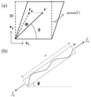
Figure 8: (a) Schematic representation of affine deformation of a two-dimensional unit cell under simple shear at a strain $\Gamma$. The initial end-to-end vector ${\bf r_{0}}$ at an angle $\Phi$ with ${\bf e}_{1}$ has transformed to a vector ${\bf r}={\bf F}{\bf r_{0}}$ at an angle $\phi$. (b) An (undulated) filament with end-to-end length $r$ at an angle $\phi$ under a tensile force $f_{\rm c}$ in the deformed state. The area $rw$ covered by the filament is, on average, constant under the assumption that the network is incompressible.

Next, the cell is subjected to a simple shear of strain $\Gamma$, by fixing the lower boundary and displacing the top boundary over a distance $W\Gamma$, see Fig. 8(a). This deformation process is represented by the deformation gradient tensor ${\bf F}$ with components

$$\left[F_{ij}\right]=\left[\begin{array}[]{cc}1&\Gamma\\ 0&1\\ \end{array}\right].$$ (39)

Note that the shear deformation process satisfies $\det{\bf F}=1$, expressing incompressibility of the filamental network.rmrkvolconservation When it is assumed that the filaments deform in an affine manner, each filament’s end-to-end vector ${\bf r_{0}}$ transforms to the vector ${\bf r}=r{\bf m}$ according to ${\bf r}={\bf F}{\bf r_{0}}$, as sketched in Fig. 8(a). Filaments thus rotate from $\Phi$ to $\phi$ and undergo a stretch of $\lambda=r/r_{0}$ that can be obtained from ${\bf F}$ through

$$\lambda^{-2}={\bf m}\left({\bf FF}^{\rm T}\right)^{-1}{\bf m},$$ (40)

where ${\bf m}={\bf r}/r=\cos\phi{\bf e}_{1}+\sin\phi{\bf e}_{2}$ is the unit vector along the filament’s end-to-end direction in the current, deformed state. From Eqs. (39) and (40) the stretch $\lambda$ can be expresssed in terms of $\phi$ and $\Gamma$ as

$$\lambda(\phi;\Gamma)=\sqrt{\frac{1+\tan^{2}\phi}{1-2\Gamma\tan\phi+(1+\Gamma^{2})\tan^{2}\phi}}.$$ (41)

A filament that is at an angle $\phi$ in the current state of shear strain $\Gamma$ is thus subjected to a stretch $\lambda$ that is given by Eq. (41). Figure 9 shows the dependence of $\lambda$ on $\phi$ for various strains $\Gamma$.

Figure 9: The stretch $\lambda=r/r_{0}$ of a filament as a function of its orientation $\phi\in[-\pi/2,\pi/2]$ in the deformed state at various levels of the shear $\Gamma$ according to Eq. (41) for affine deformation.

During shear, filaments also rotate and thus change their orientation. If $C(\phi;\Gamma)\mbox{d}\phi$ is the probability of a filament with an orientation between $\phi$ and $\phi+\mbox{d}\phi$ in the deformed state at strain $\Gamma$, it can be shown that $C(\phi;\Gamma)$ follows directly from the stretch $\lambda$ by rmrkcodf1

$$C(\phi;\Gamma)=C_{0}\lambda^{2}(\phi;\Gamma),$$ (42)

where the normalization value $C_{0}=1/\pi$ is the initial, uniform probability distribution. This probability function $C(\phi;\Gamma)$ is also known as the “chain orientation distribution function” (CODF).Wu93 ; Wu95 Figure 10 shows a polar plot of the CODF for $\Gamma=0$ and 0.30 in the angular range $[0,2\pi]$.rmrkcodf2 For $\Gamma=0$ there is no deformation and filaments are randomly distributed in the network, indicated by the spherical distribution. As the network deforms, filaments rotate in the straining direction, resulting in a nonspherical distribution, its anisotropy growing with increasing strain. For $\Gamma=0.3$ the principal directions for which a minumum and maximum stretch is obtained, are indicated by the mutually orthogonal, straight dashed lines. For this strain, filaments at an angle of $\phi=40.7$^∘undergo a maximum stretch of $\lambda=1.16$ and filaments at an angle of $\phi=-49.3$^∘  a maximum compression ($\lambda=0.86$).

Figure 10: Polar plot of the chain orientation distribution function $C(\phi;\Gamma)$ [CODF], at $\Gamma=0.0$ (solid curve) and $\Gamma=0.3$ (dashed curve). The dotted lines indicate the principal directions at $\Gamma=0.3$.

Under the assumption of affine deformation, the Eqs. (36,37,38,41,42) can be used to calculate the network response to simple shear. We start by considering an individual filament at an angle $\phi$ subjected to a stretch $\lambda(\phi,\Gamma)$ in the deformed unit cell of strain $\Gamma$, as sketched in Fig. 8(b). Assuming the network is incompressible, the area per chain, $rw$, remains constant, and is thus equal to $1/n$. The force acting on the filament, $f_{\rm c}$, can be tranformed to the Cauchy traction $\sigma_{\rm c}$ acting on the continuum in which the filament is embedded, $\sigma_{\rm c}=f_{\rm c}/(bw)$, where $w$ is the cross-sectional width and $b$ is the unit out-of-plane length the force acts on. Similar to the approach by Wu and Van der GiessenWu95 we define the micro-stress tensor $\bm{\sigma}_{\rm c}$ by

$$\bm{\sigma}_{\rm c}=\sigma_{\rm c}\left({\bf m}\otimes{\bf m}\right)-p{\bf I},$$ (43)

with $\sigma_{\rm c}=n\lambda(\phi;\Gamma)f_{\rm c}r_{0}b^{-1}$ since $r=\lambda r_{0}$. In Eq. (43) the hydrostatic stress $p$ is included to account for the incompressibility of the network. The micro-stress tensor is the contribution of a single filament oriented along $\textbf{m}(\phi)$ to the stress of the network. Finally, with the areal density of chains $\mbox{d}n$ having an orientation between $\phi$ and $\phi+\mbox{d}\phi$ given by

$$\mbox{d}n=nC(\phi;\Gamma)\mbox{d}\phi,$$ (44)

the overall or macro-stress tensor $\bm{\sigma}$ of the network can be evaluated by the average of the micro-stress tensor $\bm{\sigma}_{\rm c}$ over the individual chains in the network, i.e.,

$$\bm{\sigma}=\frac{1}{n}\int\bm{\sigma}_{\rm c}\mbox{d}n.$$ (45)

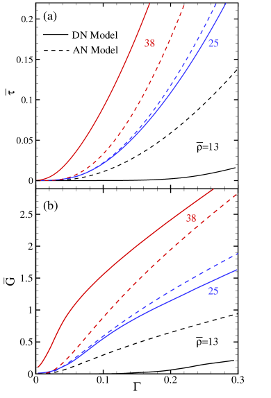
Figure 11: (a) Shear stress $\overline{\tau}$ versus shear strain $\Gamma$ response for biopolymer networks comprising filaments with $L_{\rm P}=L_{\rm C}=10~{}\mu$m, $\kappa_{\rm f}=8.53\times 10^{-17}$ Nm² and $\mu=16$ N, and (b), the corresponding shear stiffness $\overline{G}=\textrm{d}\overline{\tau}/\textrm{d}\Gamma$. Results are plotted for three filament densities: $\overline{\rho}$=13 (black curves), 25 (blue) and 38 (red). The solid curves display the results from the discrete-network (DN) calculations, the dashed curves are the results from the affine-network (AN) model, Eq. (46).

Figure 12: Shear deformation of the discrete network (DN). (a) Initial, $\Gamma=0$; (b) intermediate, $\Gamma=0.125$ and (c) large strain, $\Gamma=0.285$, network configurations for a randomly generated network of density $\overline{\rho}=13$, with $W=4L_{\rm C}=40~{}\mu\mbox{m}$.

It is important to note here that since the force acting on an individual filament depends on its end-to-end displacement, it therefore depends on its current orientation $\phi$ and applied shear strain $\Gamma$ through $f_{\rm c}(\phi;\Gamma)=f_{\rm c}(u(\phi;\Gamma))=f_{\rm c}(r_{0}(\lambda(\phi;\Gamma)-1))$.

We assume that the filaments in the network only stretch and compress upon mechanical loading, but do not bend/buckle. In Sect. III we showed that stretching by internal bending can also be neglected, and that axial stretching with stiffness $\mu/L_{\rm C}$ dominates the ensemble-averaged single-filament force-extension relation. The angular region in which stretching occurs ($\lambda\geq 1$) follows directly from Eq. (41) and is given by $\phi\in[0,\arctan(2\Gamma^{-1})]$. In this region filaments experience an elongation of their end-to-end distance; filaments outside this region are under compression ($\lambda\leq 1$) and deform by soft (internal) bending and contribute negligibly to the overall network stiffness. Hence, we adopt the force-extension relation based on Eqs. (36)–(38) in the angular region $\phi\in[0,\arctan(2\Gamma^{-1})]$. The dimensionless shear stress, $\overline{\tau}=\sigma_{12}bL_{\rm C}/\mu$, from Eqs. (42)–(45) can then be written as

$$\overline{\tau}=\frac{\overline{\rho}}{\pi\mu}\frac{\left<r_{0}\right>}{L_{\rm C}}\int\limits_{0}^{\arctan(2\Gamma^{-1})}\lambda^{3}(\phi;\Gamma)\left<f_{c}\right>(\phi;\Gamma)\sin\phi\cos\phi\mbox{d}\phi,$$ (46)

where $\overline{\rho}=\rho L_{\rm C}=N_{\rm f}\left(L_{\rm C}/W\right)^{2}$ is a dimensionless filament density. Figure 11(a) presents the calculated $\overline{\tau}$ versus $\Gamma$-curves for three densities $\overline{\rho}=$13, 25 and 38 (dashed curves). The corresponding shear stiffness, $\overline{G}=\textrm{d}\overline{\tau}/\textrm{d}\Gamma$, is shown in Fig. 11(b). As can be seen, stiffening of the network is indeed observed, resulting from the average stiffening of individual filaments in the network (Fig. 7), or said differently, stiffening results from an increase in the fraction of filaments that are stretched beyond their slack distance.

These results can be directly compared to 2D numerical discrete-network (DN) calculations using the finite-element method.OnckPRL05 Filaments of contour length $L_{\rm C}$ and persistence length $L_{\rm P}$ are randomly placed into a square cell of dimension $W$ at random orientations, with proper account of periodicity. Each filament is discretized into 15 equal-sized, Euler-Bernoulli beam elements that account for stretching (with axial stiffness $\mu$) and bending (with stiffness $\kappa_{\rm f}$). In accordance with Sect. II, 10 Fourier modes are used to describe the initial shape of the undulated filaments. The points were filaments overlap are considered to be stiff cross-links, where the rotation and the displacement of the two filaments at the cross-link is equal. Figure 12(a) shows an example of a randomly generated network of density $\overline{\rho}=13$ that is in its initial, stress-free configuration. Filaments crossing either the upper or lower boundary of the cell are perfectly bonded to rigid top and bottom plates, respectively. Next, the top plate is displaced horizontally relative to the bottom plate over a distance $\Gamma W$, corresponding to an applied shear strain of $\Gamma$. Geometry changes are accounted for by an updated Lagrangian finite-strain formulation. Figures 12(b) and (c) show the network of Fig. 12(a) in the deformed state at shears of $\Gamma$=0.125 and 0.285, respectively. The macroscopic shear stress $\tau$ is calculated from the cumulative, horizontal reaction force of nodes at the top plate, divided by the cell width $W$. Convergence studies were performed to ensure that the results are not affected by the number of elements per filament and the cell size $W$.

Figure 13: The product $\rho l_{\rm c}$ versus the filament network density $\rho$ (in $\mu\mbox{m}^{-1}$), determined from and averaged over randomly generated networks (solid squares). The dashed line indicates the limiting, high-density value of $\pi/2$. The inset shows a random network at a density of $\rho=20~{}\mu\mbox{m}^{-1}$($\overline{\rho}=200$), with $W=L_{\rm C}=10~{}\mu\mbox{m}$.

The stress-strain response (averaged over 10 different, random realizations) at three network filament densities of $\overline{\rho}=$13, 25 and 38 is included in Figure 11 (solid curves). It can be seen that, at a relatively small density ($\overline{\rho}=$13), the discrete-network (DN) calculations result in a much softer response compared to the affine-network (AN) calculations. Closer examination of the DN results reveals, first, that the small-strain mechanical response is dominated by bending and buckling of filaments,OnckPRL05 thus yielding a soft response. Second, at somewhat larger strains, filaments perform additional, nonaffine motions during shearing: filaments reorient themselves in the direction of straining by rotations and translations. These nonaffine, geometrical network reorientations can be clearly seen by comparison of Fig. 12(b) with Fig. 12(a). Both effects, bending/buckling of filaments and local network reorientations, are not taken into account in the AN model, where instead, at small strains, all filaments with an orientation between 0 and $\pi/2$ are subjected to stretch. The response in the AN model is therefore dominated by stretching of filaments, contrary to what is observed in the DN computations. However, as the strain increases, more filaments become oriented in the direction of straining, as seen in Fig. 12(c): strings of stretched filaments connect the top and bottom plate of the cell. Thus, at larger strains, the response according to the DN calculations is also dominated by stretching of filaments, which explains the stiffening in the DN curves in Fig. 11 at low densities. Since the relative amount of filaments in stretching remains small compared to that of the AN model, the stiffness determined from the DN calculations remains small compared to the stiffness from the AN model (black curves in Fig. 11).

In contrast to small densities, at larger densities (e.g., $\overline{\rho}=38$) the DN calculations exhibit a higher stiffness compared to the AN calculations (red curves in Fig. 11). The reason for this is that the cross-link density increases with filament density, with two effects. First, the higher cross-link density results in a more rigid network structure in which each filament is cross-linked to more filaments, thereby decreasing the freedom of filaments to undergo nonaffine reorientations. The transition from a bending-dominated regime to a stretching-dominated regime therefore shifts to smaller strains as can be seen by comparing the solid DN curves in Fig. 11. Second, chain segments between cross-links contain less slack than the original filaments: segments are thus stretched beyond their slack distance at smaller strains leading to a higher stiffness. In the AN model, this reduction in slack is not taken into account, but cross-links are assumed to be at the ends of the filament, independent of the density of filaments in the network. Density enters the AN model only through the prefactor in Eq. (46), which explains the (self-) similar shape of the AN curves in Fig. 11.

To correct for the decrease in slack in the AN calculations, we first have to determine the average cross-link distance, $l_{\rm c}$, in the network as a function of the density $\rho$. The values obtained from a series of generated networks are shown in Fig. 13 as the product $\rho l_{\rm c}$ versus $\rho$. The product gradually increases from $1.2950\pm 0.0325$ at $\rho=1.25~{}\mu\mbox{m}^{-1}$ ($\overline{\rho}=12.5$) to $1.5618\pm 0.0034$ at $\rho=35.0~{}\mu\mbox{m}^{-1}$ ($\overline{\rho}=350$) and thus approaches the limiting, 2D theoretical value of $\pi/2$.rmrkproduct ; HeadPRE03rc The inset shows an undeformed network with $W=L_{\rm C}=10~{}\mu\mbox{m}$ at a high density of $\rho=20.0~{}\mu\mbox{m}^{-1}$, exemplifying the short average distance between the cross-links ($l_{\rm c}=0.0775\pm 0.0003~{}\mu\mbox{m}\ll L_{\rm C}$). Next, the distribution in end-to-end lenghts $r_{0}$ of segments at a density $\rho$ is given by $\mathscr{G}(r_{0};l_{\rm c}(\rho);L_{\rm P})$ from Eq. (9), with $L_{\rm C}$ replaced by $l_{\rm c}(\rho)$. From this, the ensemble-averaged mechanical behavior of a segment of mean length $l_{\rm c}(\rho)$, i.e., $\left<G_{1}\right>(u;l_{\rm c}(\rho);L_{\rm P})$ and $\left<f_{c}\right>(u;l_{\rm c}(\rho);L_{\rm P})$, follows directly from Eqs. (37)–(38). This then serves as input for the density-corrected AN response $\overline{\tau}$ given by Eq. (46).rmrkprefactor The corrected AN response is plotted in Fig. 14 for three densities $\overline{\rho}=12.5,~{}25\mbox{ and }37.5$ (dashed curves). For comparison, the figure also displays the DN calculations from Fig. 11 (solid curves). As can be directly seen, all AN curves have gone up due the reduction in slack: already at small strains filamental segments are stretched beyond their slack distance resulting in a higher stress and stiffness. After the density correction, all AN calculations exhibit a higher stiffness than the DN calculations, irrespective of the density: as said before, this can be attributed to nonaffine network deformations (bending/buckling, local network reorientations) in the DN calculations that are not taken into account in the AN model.

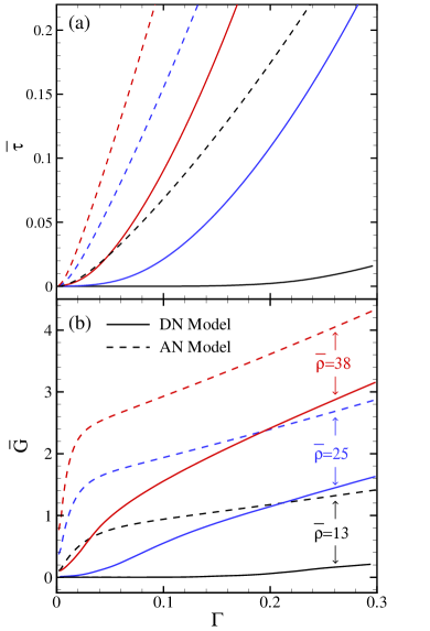
Figure 14: (a) Shear stress $\overline{\tau}$ versus shear strain $\Gamma$ response for biopolymer networks comprising filaments with $L_{\rm P}=L_{\rm C}=10~{}\mu$m, $\kappa_{\rm f}=8.53\times 10^{-17}$ Nm² and $\mu=16$ N, and (b), the corresponding shear stiffness $\overline{G}=\textrm{d}\overline{\tau}/\textrm{d}\Gamma$. Results are plotted for three filament densities: $\overline{\rho}$=12.5 (black curves), 25 (blue) and 37.5 (red). The solid curves display the results from the DN calculations (same as in Fig. 11), the dashed curves are the results from the density-corrected AN model.

In calculating the density-corrected response, the angular integration was performed in the interval $[0,\arctan(2\Gamma^{-1})]$, see Eq. (46), assuming that segments still contain a considerable amount of slack, resulting in a very compliant response in case such a segment is under axial compression. However, as discussed above, when the filament density increases, segments between cross-links become shorter and virtually straight. For a network consisting of only straight filaments, segments under compression exhibit the same axial stiffness as in tension, i.e., $\mu/l_{\rm c}$, corresponding to an axial force of $(\mu/l_{\rm c})u$. Hence, the integration should be performed over the entire angular range, $[0,\pi]$, and with the segmental force equal to $\mu[\lambda(\phi;\Gamma)-1]$, the network response is evaluated as

$$\overline{\tau}=\frac{\overline{\rho}}{\pi}\int\limits_{0}^{\pi}\lambda^{3}(\phi;\Gamma)(\lambda(\phi;\Gamma)-1)\sin\phi\cos\phi\mbox{d}\phi.$$ (47)

Eq. (47) thus gives the limiting, affine mechanical behavior of biopolymer networks of high density. Whether or not filaments are undulated and contain slack is not relevant at this point, since the segments of average length $l_{\rm c}\ll L_{\rm C}$ are straight at high densities [see inset Fig. (13)]. As we showed before, the DN calculations exhibited nonaffine deformation characteristics at low densities. However, at higher densities the DN calculations are also expected to show an affine behavior. To check this, we have investigated the initial, small-strain network stiffness, $\overline{G}_{0}$, as a function the density $\overline{\rho}$, see Fig. 15 (solid squares). The affine value follows directly from the derivative of Eq. (47) by a first-order Taylor expansion of the integrand with respect to $\Gamma$, and equalsexpansion

$$\overline{G}_{0,\rm aff}=\frac{\overline{\rho}}{8}.$$ (48)

Figure 15: Initial, small-strain stiffness $\overline{G}_{0}$ versus the density $\overline{\rho}$, calculated using the DN model (solid squares). The values of $\overline{G}_{0}$ result from an average over 10 random networks in case $\overline{\rho}<100$ and 5 networks for higher densities. The dashed line is the affine upper limit according to Eq. (48)

Note that, using the high-density limit $\rho l_{\rm c}=\pi/2$,rmrkproduct the stiffness can be rewritten as $G_{0,\rm aff}=\pi\mu/(16l_{\rm c})$, corresponding to the result found by Head et al..HeadPRL03 The normalized affine limit, $\overline{G}_{0,\rm aff}$, is included in Fig. 15 as the dashed line. It can be seen that, as the density increases, the DN calculations indeed approach the AN limit. At a density of $\overline{\rho}=350$ the DN calculations result in a stiffness of $\overline{G}_{0}=38.0\pm 0.6$, close to the affine value of 43.75.

Finally, it is interesting to see that in the networks’ stretching regime, i.e., at large strains, the network stiffness (both AN and DN) continues to increase despite the fact that the individual segments have a constant axial stiffness $\mu/l_{\rm c}$ in stretching [see Fig. 14(b)]. From this one would expect the stiffness to converge to a fixed ’steady-state’ value. However, due to nonlinear geometrical effects at large strains, the stiffness increases with straining according to

$$\overline{G}\propto\overline{\rho}~{}\Gamma^{2}(1+\Gamma^{2})^{-3/2},$$ (49)

as derived in Appendix D. From further investigation of Eq. (47) it follows that the stiffness starts to level off at very large, experimentally irrelevant strains of $\Gamma\approx 1.5$.

V Concluding remarks

We have performed a detailed investigation of the mechanical stiffening behavior of 2D semiflexible biopolymer filaments and networks of such filaments under simple shear. Such polymers undergo thermally excited bending motions, brought about by collisions with molecules of the surrounding fluid in which the filament is immersed. For inextensible filaments subjected to a tensile force, these undulations can be pulled out at the cost of an external energy input, resulting in an axial stiffness that can be calculated for two specific cases. First, we can assume no undulation dynamics to take place during tension. In this case, the filament is isolated from its surrounding fluid and the random, undulated state present in the filament is subsequently pulled out when subjected to a tensile force. In this static case, the axial stiffness results from internal bending with bending stiffness $\kappa_{\rm f}$; using equilibrium mechanics, the force-extension relation can be calculated and averaged over an ensemble of filaments. Second, undulation dynamics can be taken into account during pulling. By applying equipartition on the filament’s total energy functional at each force, the ensemble-averaged, dynamic force-extension relation can be derived. This so-called entropic stiffening was previously derived by MacKintosh and coworkers.MacKintoshPRL95

The resulting average mechanical response of single filaments in these two cases turns out to be very similar. At small forces and end-to-end displacements, both responses scale with $\kappa_{\rm f}^{2}$, with the initial dynamic stiffness being a factor 2 larger than the static one. Close to full stretching, as the average end-to-end length $\left<r\right>$ approaches the contour length $L_{\rm C}$, the force diverges as $f_{\rm c}\propto\left(L_{\rm C}-\left<r\right>\right)^{-2}$ in both models, characteristic for the worm-like chain model, with the dynamic/static stiffness ratio approaching 4. This indicates that the static and dynamic approaches are qualitatively very similar, capturing the same physical dependence on the mechanical and geometrical parameters $\kappa_{\rm f},~{}L_{\rm P}\mbox{ and }L_{\rm C}$, but differ quantitatively by a factor 2 to 4.

In case of extensible filaments of stretching stiffness $\mu$, enthalpic axial elongation dominates the filaments’ mechanical behavior close to full stretching and both models thus exhibit a quantitatively identical mechanical response. In addition, we have shown that for 2D filaments, one can very well describe the ensemble-averaged force-extension relation by completely neglecting contributions from internal bending and by merely taking into account the axial stretching of filaments and the distribution in slack.

Two-dimensional, cross-linked networks that have these semiflexible filaments as building blocks stiffen under an applied shear strain. Often, stiffening is attributed to the entropic stiffening of individual filaments undergoing affine deformations. For the 2D networks under investigation, we conclude by comparing analytical, affine network (AN) calculations with discrete (finite-element) network (DN) calculations that this cannot be the case. For networks of low filament density, the mean cross-link distance $l_{\rm c}$ is relatively large and the resulting segments between cross-links contain a relatively large amount of slack that can be pulled out. In this case, one could argue that entropic stiffening would be the main origin of stiffening. However, the DN calculations show that at these densities stiffening lies in the network rather than in its constituents: at small strains the mechanical response is dominated by bending/buckling of filaments and nonaffine rotations and translations. These local network rearrangements induce a transition from a bending-dominated regime at small strains to a stretching-dominated regime at larger strains in which strings of connected filaments dominate the mechanical response. At higher network densities, the number of cross-links increases and the mean cross-link distance $l_{\rm c}$ decreases, so that the shorter segments between cross-links contain less slack. The higher network density then results in a mechanical response that is more affine in nature, with the mentioned reduction in slack increasing the enthalpic stretching contribution of the segments. By accounting for the reduced slack in the AN calculations, the DN results were severely overestimated, showing that, for the densities investigated, the discrete-network architecture plays a key role. Only in the limit of extremely high densities do the DN and reduced-slack AN calculations coincide.

Hence, we conclude that, for physiological relevant densities, stiffening in 2D networks results from nonlinearities in the network response, rather than from entropic stiffening of individual filaments. Note that these conclusions might be different for three-dimensional networks, since the amount of slack in filaments is significantly higher than in 2D. Current work focuses on this issue in 3D networks.

Appendix A

While real semiflexible filaments are, evidently, three-dimensional objects that are often idealized as rods of diameter $d$, 2D models require some ’projected’ thickness $t$ for the specification of the axial and the flexural stiffness in terms of Young’s modulus $E$, the area of a filament’s cross section, $A$, and its second moment of inertia, $I$. This ’projection’, however, is not trivial nor unique. While the moment of inertia of a circular cross-section of diameter $d$ is $I=\pi d^{4}/64$, that of a projected filament with thickness $t$ is $I=bt^{3}/12$ with some out-of-plane width $b$. Aiming at actin filaments which typically have a diameter of $d=8$ nm, we use 2D filaments with $t=8$ nm. When a typical value of $E=2$ GPa is used for the Young’s modulus of actin, the bending stiffness $\kappa_{\rm f}$ of such 2D filaments with a unit out-of-plane thickness (i.e., $b=1$ m) is

$$\kappa_{\rm f}=EI=E\frac{bt^{3}}{12}\approx 8.53\times 10^{-17}~{}\mbox{Nm}^{2}.$$ (50)

If we would use this result in Eq. (2), the persistence length would be $2.1\times 10^{4}$ m, much larger than the contour length $L_{\rm C}$ and filaments would simply be straight, which they are not in 3D. Therefore, the persistence length is scaled back to the contour length (scale factor: $4.8\times 10^{-10}$) to generate semiflexible filaments for which $L_{\rm P}=L_{\rm C}=10~{}\mu$m, as described in section II.

For the calculations performed in sections II, III, and IV we use the same input value of $L_{\rm P}=10~{}\mu$m to generate the undulated filaments (i.e., the initial configurational state {$a_{n}^{0}$}, determined by this value of $L_{\rm P}$) , but for the bending stiffness $\kappa_{\rm f}$ in the beam-equation [Eq. (12)] we use the value calculated in Eq. (50). For this reason $L_{\rm P}$ and $\kappa_{\rm f}$ are treated as separate parameters in the eqs. (21)–(26). With the same 2D representation as underlying Eq. (50), the value of the stretching stiffness $EA$ is

$$\mu=EA=Ebt\approx 16~{}\mbox{N}.$$ (51)

Appendix B

For a Gaussian distribution with mean $\left<a_{n}^{0}\right>=0$ and standard deviation $s_{n}$ , the probability $p(a_{n}^{0})\mbox{d}a_{n}^{0}$ of finding a mode amplitude between $a_{n}^{0}$ and $a_{n}^{0}+\mbox{d}a_{n}^{0}$ is

$$p(a_{n}^{0})\mbox{d}a_{n}^{0}=\frac{1}{\sqrt{2\pi s_{n}^{2}}}\exp\left[-\frac{\left(a_{n}^{0}\right)^{2}}{2s_{n}^{2}}\right]\mbox{d}a_{n}^{0}.$$

The mean-squared value of $a_{n}^{0}$ is given by

$$\left<\left(a_{n}^{0}\right)^{2}\right>=\int_{-\infty}^{\infty}\left(a_{n}^{0}\right)^{2}p(a_{n}^{0})\mbox{d}a_{n}^{0}=s_{n}^{2}.$$

Using Eq. (21) resulting from equipartition of the internal bending energy, the standard deviation is given by

$$s_{n}=\sqrt{\left<\left(a_{n}^{0}\right)^{2}\right>}=\sqrt{\frac{1}{L_{\rm P}}}q_{n}^{-1}~{}~{}~{}\mbox{(for $n\geq 1$)}.$$

Appendix C

In the absence of an externally applied force, a 2D semiflexible filament characterized by the tangent angle $\theta$

$$\theta(s,\{a_{n}^{0}\})=\sqrt{\frac{2}{L_{\rm C}}}\sum_{n\geq 1}a_{n}^{0}\cos\left[q_{n}s\right],$$ (C-1)

is in a configurational state denoted by {$a_{n}^{0}$}. The probability of a filament being in a state between {$a_{n}^{0}$} and d{$a_{n}^{0}$} is

$$p(\{a_{n}^{0}\})\textrm{d}\{a_{n}^{0}\}=\frac{1}{Z}\exp\left[-\frac{\mathscr{H}_{B}(\{a_{n}^{0}\})}{k_{B}T}\right]\prod_{n\geq 1}\textrm{d}a_{n}^{0},$$ (C-2)

where $\textrm{d}\{a_{n}^{0}\}\equiv\prod_{n\geq 1}\textrm{d}a_{n}^{0}$, $Z$ is the partition function given by

$$Z=\int_{-\infty}^{\infty}\ldots\int_{-\infty}^{\infty}\exp\left[-\frac{\mathscr{H}_{B}(\{a_{n}^{0}\})}{k_{B}T}\right]\prod_{n\geq 1}\textrm{d}a_{n}^{0},$$ (C-3)

and $\mathscr{H}_{B}$ is the internal bending energy of the filament given by Eq. (20). After substituting the Fourier series for $\theta$ into $\mathscr{H}_{B}$ and by using $\sin\theta\approx\theta$, one finds

$$\frac{\mathscr{H}_{B}(\{a_{n}^{0}\})}{k_{\rm B}T}=\frac{L_{\rm P}}{2}\sum_{n\geq 1}q_{n}^{2}(a_{n}^{0})^{2}.$$ (C-4)

This result can be substituted into Eq. (C-3) yielding the partition function

$$Z=\prod_{n\geq 1}~{}\int\limits_{-\infty}^{\infty}\exp\left[-\frac{L_{\rm P}}{2}q_{n}^{2}(a_{n}^{0})^{2}\right]\textrm{d}a_{n}^{0}=\prod_{n\geq 1}\left(\frac{2\pi}{L_{\rm P}q_{n}^{2}}\right)^{1/2}.$$ (C-5)

The ensemble-average of a quantity $A(\{a_{n}^{0})\})$ is defined by

$$\left<A\right>=\int\limits_{-\infty}^{\infty}\ldots\int\limits_{-\infty}^{\infty}p(\{a_{n}^{0})\})A(\{a_{n}^{0})\})\prod_{n\geq 1}\textrm{d}a_{n}^{0}$$ (C-6)

The end-to-end distribution function can be calculated by the following ensemble averageWilhelmPRL96

$$\mathscr{G}(r_{0})=\left<\delta\left(r_{0}-\left[L_{\rm C}-\frac{1}{2}\sum_{n\geq 1}(a_{n}^{0})^{2}\right]\right)\right>,$$ (C-7)

where $\delta(r_{0})$ is the Dirac delta function, and $L_{\rm C}-\frac{1}{2}\sum_{n\geq 1}(a_{n}^{0})^{2}$ is the end-to-end distance of the chain in the absence of an externally applied force ($f_{c}=0$), according to Eq. (16). Next, we can combine Eqs. (C-2,C-4-C-7) and make use of the following property of the delta function

$$\delta(r_{0})=\frac{1}{2\pi}\int\limits_{-\infty}^{\infty}\exp[izr_{0}]\textrm{d}z,$$

resulting in the following integral solution for $\mathscr{G}(r_{0})$:

$$\mathscr{G}(r_{0})=\frac{1}{2\pi}\int\limits_{-\infty}^{\infty}\textrm{d}z\exp\left[iz(r_{0}-L_{\rm C})\right]\prod_{n\geq 1}\left(\frac{L_{\rm P}q_{n}^{2}}{L_{\rm P}q_{n}^{2}-iz}\right)^{1/2}$$ (C-8)

Next, we rewrite the product inside the integral expression as

$$\prod_{n\geq 1}\left(\frac{L_{\rm P}q_{n}^{2}}{L_{\rm P}q_{n}^{2}-iz}\right)^{1/2}=\exp\left[\frac{1}{2}\psi(iz)\right],$$ (C-9)

in which $\psi$ is defined as

$$\psi(z)=\sum_{n\geq 1}\ln\left(\frac{L_{\rm P}q_{n}^{2}}{L_{\rm P}q_{n}^{2}-z}\right)$$

The derivative $\mbox{d}\psi/\mbox{d}z$ can be written as

$$\frac{\mbox{d}\psi(z)}{\mbox{d}z}=\sum_{n\geq 1}\frac{1}{L_{\rm P}q_{n}^{2}-z}=\frac{1}{2z}\left[1-\sqrt{\frac{zL_{\rm C}^{2}}{L_{\rm P}}}\cot\sqrt{\frac{zL_{\rm C}^{2}}{L_{\rm P}}}\right],$$

and integrated to yield (with $\psi(0)=0$)

$$\psi(z)=\ln\left(\frac{\sqrt{zL_{\rm C}^{2}/L_{\rm P}}}{\sin\sqrt{zL_{\rm C}^{2}/L_{\rm P}}}\right).$$ (C-10)

Equations (C-9,C-10) are subsituted into Eq. (C-8), and by substitution of variables accoring to $z=iL_{\rm P}\omega^{2}$ we eventually arrive to

$$\mathscr{G}(r_{0})=\frac{L_{\rm P}}{2\pi i}\int\limits_{-i\infty}^{i\infty}\textrm{d}\omega\exp\left[-\omega^{2}L_{\rm P}(r_{0}-L_{\rm C})\right]$$

$$\times~{}2\omega\left(\frac{\omega L_{\rm C}}{\sinh(\omega L_{\rm C})}\right)^{1/2}$$ (C-11)

Next, we can use the binomial expansionbinomial to expand the inverse square root of $\sinh(\omega L_{\rm C})$

$$\sinh(\omega L_{\rm C})^{-\textstyle{\frac{1}{2}}}=\sqrt{2}\sum_{k\geq 0}{-\textstyle{\frac{1}{2}}\choose k}(-1)^{k}\exp\left[-(2k+\textstyle{\frac{1}{2}})\omega L_{\rm C}\right].$$

The distribution function then becomes

$$\mathscr{G}(r_{0})=\frac{L_{\rm P}\sqrt{2L_{\rm C}}}{\pi i}\sum_{k\geq 0}{-\frac{1}{2}\choose k}(-1)^{k}\int\limits_{-i\infty}^{i\infty}\textrm{d}\omega\omega^{\frac{3}{2}}$$

$$\times~{}\exp\left[-\omega^{2}L_{\rm P}(r_{0}-L_{\rm C})-(2k+\frac{1}{2})\omega L_{\rm C}\right]$$ (C-12)

We can rewrite Eq. (C-12) using so-called parabolic cylinder functions $D_{\nu}(z)$, defined byAbramowitz

$$D_{\nu}(x)=\frac{1}{\sqrt{2\pi}i}\exp\left[\frac{x^{2}}{4}\right]\int\limits_{-i\infty}^{i\infty}s^{\nu}\exp\left[-xs+\frac{1}{2}s^{2}\right]\textrm{d}s.$$ (C-13)

Using the following substitution of variables,

$$s=\omega\sqrt{2L_{\rm P}(L_{\rm C}-r_{0})}\mbox{, and }x=\frac{2(k+1/4)L_{\rm C}}{\sqrt{2L_{\rm P}(L_{\rm C}-r_{0})}},$$

the distribution function is rewritten as (with $\nu=3/2$)

$$\mathscr{G}(r_{0})=\frac{2L_{\rm P}\sqrt{L_{\rm C}}}{\sqrt{\pi}}\sum_{k\geq 0}{-\frac{1}{2}\choose k}(-1)^{k}\frac{1}{[2L_{\rm P}(L_{\rm C}-r_{0})]^{5/4}}$$

$$\times~{}\exp\left[-\frac{(k+\frac{1}{4})^{2}L_{\rm C}^{2}}{2L_{\rm P}(L_{\rm C}-r_{0})}\right]D_{3/2}\left[\frac{2(k+\frac{1}{4})L_{\rm C}}{\sqrt{2L_{\rm P}(L_{\rm C}-r_{0})}}\right]$$

(C-14)

Finally, we can rewrite the binomial coefficient in terms of the Gamma function:

$${-\frac{1}{2}\choose k}=\frac{\Gamma\left(\frac{1}{2}\right)}{\Gamma(k+1)\Gamma\left(\frac{1}{2}-k\right)},$$

with $\Gamma(k+1)=k!$. By making use of the following identity of the Gamma function

$$\Gamma\left(n+\frac{1}{2}\right)=\frac{(2n-1)!!}{2^{n}}\Gamma\left(\frac{1}{2}\right),$$

substituting $n=-k$ and the identity

$$(-2k-1)!!=\frac{(-1)^{k}}{(2k-1)!!},$$

we arrive at the the following expression for the binomial coefficient

$${-\frac{1}{2}\choose k}=\frac{(2k-1)!!}{2^{k}k!}(-1)^{k}.$$

The distribution function is therefore written as

$$\mathscr{G}(r_{0})=\frac{2L_{\rm P}\sqrt{L_{\rm C}}}{\sqrt{\pi}}\sum_{k\geq 0}\frac{(2k-1)!!}{2^{k}k!}\frac{1}{[2L_{\rm P}(L_{\rm C}-r_{0})]^{5/4}}$$

$$\times~{}\exp\left[-\frac{(k+\frac{1}{4})^{2}L_{\rm C}^{2}}{2L_{\rm P}(L_{\rm C}-r_{0})}\right]D_{3/2}\left[\frac{2(k+\frac{1}{4})L_{\rm C}}{\sqrt{2L_{\rm P}(L_{\rm C}-r_{0})}}\right]$$

Appendix D

We consider a ‘network’ consisting of parallel filament strings that are initially normal to the plane of shear, separated by a distance $H$ [see dashed lines in sketch(a)]. The strings have a stretching stiffness $\mu$ and connect the top and bottom plates separated by a distance $W$. Next, the network is subjected to a shear of strain $\Gamma$ by displacing the top plate by a distance $u$. Strings rotate by an angle $\beta=\arctan\left(\Gamma\right)$ and undergo a stretch, leading to a certain shear stress $\tau$.

The instantenous stiffness $G$ can be found by increasing the top-plate displacement from $u\mbox{ to }u+\Delta u$ [see sketch(b)] corresponding to a increase $\Delta\Gamma$ in strain and resulting in an increase $\Delta\tau$ in stress. Using a unit out-of-plane dimension, the shear stiffness is defined as

$$G=\frac{\Delta\tau}{\Delta\Gamma}=\frac{W}{H}\frac{\Delta P_{x}}{\Delta u},$$ (D-1)

in which $\Delta P_{x}$ is the increase in string’s force ($\Delta P$) projected on the shearing direction, i.e., $\Delta P_{x}=\Delta P\sin\beta$. The linear response of each string,

$$\Delta P=\mu\frac{\Delta L}{L},$$ (D-2)

in terms of its elongation $\Delta L$, along with the geometrical relations $\Delta L=\Delta u\sin\beta$ and $L=u/\sin\beta$, yields

$$\Delta P_{x}=\mu\frac{\Delta u}{u}\sin^{3}\beta.$$ (D-3)

Inserting Eq. (D-3) into Eq. (D-1) and using $u=W\tan\beta$, we arrive at

$$G=\frac{\mu}{H}\sin^{2}\beta\cos\beta.$$ (D-4)

Finally, since the distance between strings is inversely proportional to the network’s line density, i.e., $H\propto\rho^{-1}$, and by employing $\beta=\arctan(\Gamma)$ we obtain at the following scaling relation for the stiffness

$$G\propto\rho\mu\frac{\Gamma^{2}}{(1+\Gamma^{2})^{3/2}}\,.$$ (D-5)

References

- (1) N. Wang and D.E. Ingber, Biochemistry and Cell Biology, 73, 327–335 (1995).
- (2) M.L. Gardel, J.H. Shin, F.C. MacKintosh, L. Mahadevan, P. Matsudaira, D.A. Weitz, Science 304, 1301 (2004).
- (3) J. Xu, Y. Tseng, D. Wirtz, J. Biol. Chem. 275, 35886 (2000).
- (4) Y. Tseng, K.M. An, O. Esue, D. Wirtz, J. Biol. Chem. 279, 1819 (2004).
- (5) P.A. Janmey, U. Euteneuer, P. Traub and M. Schliwa, J. Cell Biol. 113, 155 (1991).
- (6) L. Ma, J. Xu, P.A. Coulombe and D.J. Wirtz, J. Biol. Chem. 274, 19145 (1999).
- (7) J.F. Leterrier, J. Käs, J. Hartwig, R. Vegners, P.A. Janmey, J. Biol. Chem. 271, 15687 (1996).
- (8) M.D. Bale, J.D. Ferry, Thromb. Res. 52, 565 (1988).
- (9) P.A. Janmey, E. Amis, J. Ferry, J. Rheol. 27, 135 (1983).
- (10) D.H. Wachsstock, W.H. Schwartz, and T.D. Pollard, Biophys. J. 66, 801 (1994).
- (11) B. Wagner, R. Tharmann, I. Haase, M. Fischer, and A.R. Bausch, Proc. Natl. Acad. Sci. USA 103, 13974 (2006).
- (12) M.L. Gardel, F. Nakamura, J.H. Hartwig, J.C. Crocker, T.P. Stossel, and D.A. Weitz, Proc. Natl. Acad. Sci. USA 103, 1762 (2006).
- (13) B.A. DiDonna and A.J. Levine, Phys. Rev. Lett. 97, 068104 (2006).
- (14) J.L. McGrath, Current Biology 16, R326 (2006).
- (15) R. Tharmann, M.M.A.E Claessens, and A.R. Bausch, submitted.
- (16) F.C. MacKintosh, J. Käs and P.A. Janmey, Phys. Rev. Lett. 75, 4425 (1995).
- (17) D.A. Head, A.J. Levine and F.C. MacKintosh, Phys. Rev. Lett. 91, 108102 (2003).
- (18) D.A. Head, A.J. Levine and F.C. MacKintosh, Phys. Rev. E 68, 061907 (2003).
- (19) J. Wilhelm and E. Frey, Phys. Rev. Lett. 91, 108103 (2003).
- (20) A.J. Levine, D.A. Head, and F.C. MacKintosh, J. Phys.: Condens Matter 16, s2079 (2004).
- (21) B.A. DiDonna and T.C. Lubensky, Phys. Rev. E 72, 066619 (2005).
- (22) C. Storm, J.J. Pastore, F.C. MacKintosh, T.C. Lubensky, and P.A. Janmey, Nature 435, 191 (2005).
- (23) C. Heussinger and E. Frey, Phys. Rev. Lett. 97, 105501 (2006).
- (24) K. Kroy and E. Frey, Phys. Rev. Lett. 77, 306 (1996).
- (25) T. Odijk, Macromolecules 16, 1340 (1983).
- (26) X. Liu and G.H. Pollack, Biophys. J. 83, 2705 (2002).
- (27) P.D. Wu and E. van der Giessen, J. Mech. Phys. Solids 41, 427 (1993).
- (28) P.R. Onck, T. Koeman, T. van Dillen, and E. van der Giessen, Phys. Rev. Lett. 95, 178102 (2005).
- (29) Howard, J., Mechanics of motor proteins and the cytoskeleton (Sinauer Associates, Inc., Sunderland, Massachusetts, 2001).
- (30) F. Gittes, B. Mickey, J. Nettleton, and J. Howard, J. Cell Biol. 120, 923 (1993).
- (31) In principle , which we will use in this paper’s anlytical calculations. We will show, however, that the shape of a filament can be described well by -values on the order of ten.
- (32) As can be seen from Fig. 2 the filament does not exactly end on the -axis due to the approximation made in Eq. (6). Therefore, the (small) value of is also taken into account in calculating the end-to end distance.
- (33) J. Wilhelm and E. Frey, Phys. Rev. Lett. 77, 2581 (1996).
- (34) The adjective ‘static’ here signifies that only the initial, undulated configuration is taken into account (no undulation dynamics).
- (35) This follows directly from Eq. (19): close to full stretching approaches , resulting in and hence a stiffness of .
- (36) Based on Eq. (7), we can use the following approximation for semiflexible filaments: with . Taylor expansion in yields . The average slack is therefore .
- (37) J.F. Marko, E.D. Siggia, Macromol. 28, 8759 (1995).
- (38) Here and in the sequel, the superposed tilde denotes quantities in the dynamic description.
- (39) P.D. Wu and E. van der Giessen, Phil. Mag. A 71, 1191 (1995).
- (40) An initial volume element subjected to a deformation process characterized by the strain gradient tensor , changes its volume to . Volume conservation is thus expressed by .
- (41) This is similar to the general expression of the chain-orientation-distribution-function (CODF) in three dimensions (with spherical angles and ) which reads with , as derived by Wu and Van der Giessen. Wu93 ; Wu95
- (42) Note that the CODF is a periodic function of period . Therefore the normalization in Eq. (42) is done over an angular range of , e.g. or , but the CODF is plotted here over the whole angular range of .
- (43) This limiting value can be obtained by considering straight filaments of length , oriented at random angles with the x-axis, in a square cell of dimension . The probability of a filament intersecting the x-axis is simply . The probability of this filament intersecting a filament aligned with the x-axis is thus . The average cross-link probability can be found by averaging over the angle and results in . In the high-density limit, the mean number of cross-links per filament, , is simply the product of the average cross-link probability and number of filaments, i.e., . Using , this results in the high-density limit .HeadPRE03rc
- (44) D.A. Head, F.C. MacKintosh, and A.J. Levine, Phys. Rev. E 68, 025101(R) (2003).
- (45) Note that the prefactor in Eq. (46) changes to , with the average end-to-end distance of a segment. However, the dimensionless quantities and are still defined as and , respectively.
- (46) First-order Taylor expansion of the integrand in Eq. (47) in terms of : , resulting in .
- (47) which holds for all complex with .
- (48) M. Abramowitz and I.A. Stegun, Handbook of mathematical functions (Dover Publ., New York, 1965).