Notes on statistical separation of classes of events

Introduction

A common problem is that of separating different classes of events in a given sample. One may want to separate some ”signal” from one or more ”background” sources, or simply distinguish between different classes of signal events. There are several instances where one cannot or does not wish to separate by means of cutting, and instead wants to do a statistical separation. This means to be able to calculate the number of events in each category that are present in the given sample, and maybe measure some other characteristics of each class, without explicitly labeling each individual event as belonging to a particular category. For this to be possible, one needs some observables that have different distributions for each class of events.

The purpose of this note is to define some criteria for quantifying the resolution achievable in statistical separation, given the distributions of the observables used to this purpose. One can use this to:

• quote the separation power of an observable in a compact way

• quickly evaluate the expected resolution on extracting the fractions of events in each category before actually performing any fit

• decide the optimal variables to use in separation when there are several choices

Separating contributions

Suppose your sample contains $n$ different classes of events, each contributing a fraction $f_{i}$ of the total, and let $x$ be some observable (which may be multidimensional) that is supposed to distinguish between those events. The probability distribution of $x$ for our sample will be:

$$p_{tot}(x|f)=\sum_{i=1,n}{f_{i}p_{i}(x)}$$ (1)

where $p_{i}(x)$ is the pdf of $x$ for events of type $i$, and it is assumed here to be perfectly known (any uncertainty in the $p_{i}(x)$ would contribute a systematic uncertainty to the final results).

The most basic informations one wishes to extract from the sample of data at hand is the values of the fractions $f_{i}$; we can therefore take the resolution in extracting the $f_{i}$’s as the measure of the separating power of the observable $x$.

The sum of all $f_{i}$ must be 1 in order for the overall distribution to be correctly normalized, so there are actually only $n-1$ free parameters to be evaluated; let’s put arbitrarily $f_{n}=1-\sum_{i=1,n-1}{f_{i}}$.

The resolution in estimating the $f_{i}$’s can in principle be measured by setting up a Maximum Likelihood fit procedure, and repeating it on a sufficient number of MonteCarlo samples to evaluate the spread of results around the input values. You can also look at the resolutions returned by your favorite fitter program, but it is important to remember that those numbers are only approximate estimates of the actual resolution achieved, especially when statistics is low and/or the likelihood function is less than regular, so it is useful to be able to calculate them indipendently. This is also a good cross–check that the fit is actually doing what you want and that its error estimates are sound.

A standard way to evaluate the resolution expected from a measurement before actually carrying it out is to look at the Minimum Variance Bound[1]:

$$cov(\hat{\mu_{i}},\hat{\mu_{j}})=-\left[E\left[\frac{\partial^{2}{\log{\cal L}}}{\partial{\mu_{i}}\partial{\mu_{j}}}\right]\right]_{ij}^{-1}$$ (2)

this is an upper bound to the precision that can be achieved, whatever the estimation procedure used. Whenever the problem is sufficiently regular, the ML estimator gets in fact very close to this limit.

Luckily enough, the MVB for our problem can be written down in a pretty simple form: the covariance matrix of the $n-1$ independent $f_{i}$ parameter estimates is:

$$cov(f_{i},f_{j})=\frac{1}{N}\left[\int\frac{\left(p_{i}(x)-p_{n}(x)\right)\,\left(p_{j}(x)-p_{n}(x)\right)}{p_{tot}(x|f)}\,dx\right]_{ij}^{-1}$$ (3)

(remember that the fraction $f_{n}$ associated to distribution $p_{n}(x)$ is determined from the other $f_{i}$’s). Note that in this formula the symbol $x$ may stand for a set of many variables, discrete and/or continuous, and the integrals extend over the whole $x$ domain.

For a 2–component sample, there is only one fraction $f=f_{1}$ to be evaluated, and the result is particulary simple:

$$\sigma^{2}(f)=\frac{1}{N}\left(\int\frac{{\left(p_{1}(x)-p_{2}(x)\right)}^{2}}{fp_{1}(x)+(1-f)p_{2}(x)}\,dx\right)^{-1}$$ (4)

This is the quantity you want to minimize in order to achieve the best possible statistical separation.

In the limiting case of the different classes of events being totally separated in $x$, that is, the $p_{i}(x)$ having zero overlap, the uncertainties on $f_{i}$ come just from the statistical fluctuations of the distribution of the events amongst classes due to finite sample size, and eq. 4 becomes:

$$\sigma_{best}^{2}(f)=\frac{f(1-f)}{N}$$ (5)

which is the familiar result from the Binomial distribution.

It is particularly convenient to use the ratio of the resolution (4) to the limit resolution (5), in order to quote the separation power of the observable $x$ as an adimensional quantity:

$$s=\sigma_{best}(f)/\sigma(f)=\sqrt{f(1-f)\int\frac{\left(p_{1}(x)-p_{2}(x)\right)^{2}}{p_{tot}(x|f)}\,dx}$$ (6)

This is indipendent from the sample size $N$, and tells you at a glance the power of the $x$ observable in separating the samples, from $0$ (no separation) to $1$ (absolute maximum achievable with the given sample). This quantity is more informative than common expressions like ”$n$-sigma separation” or ”curves overlap by $xxx$%”, as it tells you exactly how good the observable $x$ is in separating the events, and it is valid whatever the shape and the dimensionality of the distributions involved.

Examples

A simple and common example is the separation between two 1-dimensional gaussian distributions of same sigma. The above quantity $s$ is easily evaluated by numerical integration. Note that $s$, as it generally happens for resolutions, depends on the true value of the fractions $f_{i}$. Figure 1 shows $s$ as a function of the distance, in units of sigma, between the mean values of the two gaussians, and the different curves are for different values of $f$. From this graph you can read, for instance, that a separation of 1 sigma between roughly equally populated samples gives you a resolution on the relative fractions slightly more than a factor of two ($1/0.45$) worse than ideal, that is to say, the sample is statistically equivalent to a fully separated sample of size smaller by a factor $0.2=0.45^{2}$.

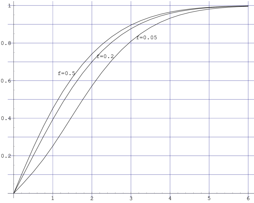
Figure 1: Separation power between two gaussians, as a function of their distance

References

- [1] This is discussed in most statistics book, see for instance: W. T. Eadie, D. Drijard, F. E. James, M. Roos, and B. Sadoulet,Statistical Methods in Experimental Physics (North-Holland, Amsterdam, 1971).