A volume-based description of gas flows with localised mass-density variations

Abstract

We reconsider some fundamental aspects of the fluid mechanics model, and the derivation of continuum flow equations from gas kinetic theory. Two topologies for fluid representation are presented, and a set of macroscopic equations are derived through a modified version of the classical Boltzmann kinetic equation for monatomic gases. The free volumes around the gaseous molecules are introduced into the set of kinetic microscopic parameters. Our new description comprises four, rather than three, conservation equations; the classical continuity equation, which conflates actual mass-density and number-density in a single equation, has been split into a conservation equation of mass (which involves only the classical number-density of the gaseous particles) and an evolution equation purely of the mass-density (mass divided by the actual volume of the fluid). We propose this model as a better description of gas flows displaying non-local-thermodynamic-equilibrium (rarefied flows), flows with relatively large variations of macroscopic properties, and/or highly compressible fluids/flows.

, and

1 Introduction

In rarefied gas dynamics, the Boltzmann kinetic equation is accepted as describing the evolution of the gaseous particle distribution function. This equation is presumed to be valid for any dilute gas flow, and various kinetic models have been developed as approximations to it. The most well-known are the BGK relaxation model [1], the Chapman-Enskog perturbation method [2], the Linearized Boltzmann equation with polynomial decompositions [3], and the Grad moments method with Maxwellian weighting function [4], as well as more recent extensions and developments of these models. All these kinetic models lead to the set of three hydrodynamic equations, usually called the Navier-Stokes equations, that have amply demonstrated their success in describing typical engineering flows with relatively small density variations. However, the description of flows beyond the broad range of applicability of the Navier-Stokes model (such as hypersonic flows, or micro- or nano-scale gas flows) remains an active area of investigation.

The appropriateness of the Navier-Stokes model for a gas flow rests on there being sufficient local homogeneity in the flow such that macroscopic variables (e.g. mass-density, temperature, pressure etc.) are locally relatively uniform, with only small departures from thermodynamic equilibrium. In this case, a local Maxwellian representation can be assumed in approximating the solution to the Boltzmann equation. Departures of the real distribution function of the gaseous particles from the local Maxwellian are assumed to be only slight. This assumption is acceptable if the following condition is satisfied by the macroscopic flow properties:

$$\left|\frac{d\Phi}{\Phi}\right|\ll 1,$$ (1)

where $\Phi$ is a flow macroscopic property. If condition (1) does not hold then one or more macroscopic properties admit large relative variation, and the distribution function cannot be safely assumed to depart only slightly from a local equilibrium. The above assumptions and condition (1) play a key role in the various kinetic models. Flows with large relative variations in their macroscopic properties are not well understood (see, e.g., [5, 6]) although there have been numerous attempts to develop hydrodynamic models for this class of flows: see, e.g., [7, 8, 9, 10].

In this paper we introduce a new treatment for fluids and flows that are sensitive to relative variations of macroscopic flow properties. We first examine the topological representations of gases and thereby attempt a rigorous definition of both “mass-velocity” and “volume-velocity”. We then derive from the fundamental kinetic theory the set of conservation equations corresponding to a volume-representation of fluids. While this approach owes much to the recent work of Howard Brenner [11, 12] and Hans Christian Öttinger [13, 14] questioning the conventional fluid mechanical description, our focus here is on putting the volume-representation of gases on a more rigorous footing that is rooted in the fundamental kinetic theory.

2 The topology of fluid representation

A fluid is composed of a great number of molecules occupying a given volume in physical space. In the case of a gas, the physical volume occupied by the gaseous molecules can be regarded as the envelope of the physical domain occupied by the gas, and this can be represented geometrically. In a fixed reference frame this envelope may vary: for example, the gas may expand or contract.

In this section we present two different topological spaces for representing gases. The first is based on the individual point-mass particles, and the second representation is based on the geometrical envelope of the gas in physical space (i.e. the volume in which a number of gaseous molecules is dispersed). These two topological spaces are two basically different measures (or integration forms). Associated with each are essentially different ways to perform balances.

2.1 “Mass-based representation” and the measure defined by
an element of mass

A gas may be regarded as discrete point-mass particles (the gaseous molecules) distributed in physical space. Disregarding the shape of the geometrical domain occupied by the group of particles, we are only concerned with the number of point-mass particles.

A set, $\Xi_{m}$, is defined by the discrete (numerated) molecules. Any open subset, $\Omega$, represents a prescribed number of molecules. The set of whole subsets, $\Omega$, of $\Xi_{m}$ will be denoted $\Lambda_{m}$. We may define the following application:

$$\Lambda_{m} \rightarrow \mathcal{R^{+}},$$ (2)

$$\Omega \mapsto \mathrm{Mes}_{m}(\Omega),$$

where $\mathrm{Mes}_{m}(\Omega)=M\times n_{\Omega}$, with $M$ the molecular mass and $n_{\Omega}$ the number of point-mass molecules represented by $\Omega$. Then $\mathrm{Mes}_{m}(\Omega)$ is the total measurable mass of the molecules contained in $\Omega$. This application defines a measure on the topological space $(\Xi_{m},\Lambda_{m})$. For any two different open subsets, $\Omega_{i}$ and $\Omega_{j}$ in $\Lambda_{m}$, so that $\Omega_{i}\cap\Omega_{j}=\O$, we have

$$\mathrm{Mes}_{m}(\Omega_{i})+\mathrm{Mes}_{m}(\Omega_{j})=m_{i}+m_{j}\ ,$$ (3)

where $m_{i}$ (or $m_{j}$) is the mass constituting the element $\Omega_{i}$ (or $\Omega_{j}$).

2.2 “Volume-based representation” and the measure defined by
an element of volume

Instead of regarding only the point-mass particles, we might be concerned with the physical domain occupied by these dispersed particles. A prescribed number of molecules occupy a given volume in physical space. This volume can be regarded as the geometrical envelope of this group of molecules. Considering a gas in motion at a given time, $t$, the domain occupied by the group of gaseous molecules can be split among the point-mass particles according to their real position at this time $t$ (see figure 1). So each gaseous particle is attributed a microscopic fractional volume of the total volume occupied by the group of molecules.

As a “volume of fluid” means the physical volume occupied by an ensemble of gaseous molecules, the microscopic volume attributed to each particle in this description can be read as a “microscopic volume of fluid”. Each microscopic volume contains only one molecule, and the whole volume of fluid is given by the summation over all microscopic volumes. In this second fluid topological description, a prescribed “amount of fluid” or a “volume of fluid” means “a number of microscopic volumes”.

A set, $\Xi_{v}$, is defined by the microscopic volumes. Any open subset, $\Omega$, represents a prescribed number of microscopic volumes. The set of these subsets $\Omega$ of $\Xi_{v}$ will be denoted $\Lambda_{v}$. We may define the following application:

$$\Lambda_{v} \rightarrow \mathcal{R^{+}},$$ (4)

$$\Omega \mapsto \mathrm{Mes}_{v}(\Omega),$$

where $\mathrm{Mes}_{v}(\Omega)$ is the measurable value of the geometrical volume represented by $\Omega$. This application defines a measure on the topological space $(\Xi_{v},\Lambda_{v})$. It should be noted that, according to the microscopic volume distribution (see also figure 1), the elementary microscopic geometrical volumes are such that, for a couple of microscopic volumes $\Omega_{i}$ and $\Omega_{j}$,

$$\Omega_{i}\cap\Omega_{j}=\O.$$ (5)

This ensures the measure additivity property. Therefore, for two different open subsets, $\Omega_{i}$ and $\Omega_{j}$ in $\Lambda_{v}$, so that $\Omega_{i}\cap\Omega_{j}=\O$, we have

$$\mathrm{Mes}_{v}(\Omega_{i})+\mathrm{Mes}_{v}(\Omega_{j})=v_{i}+v_{j},$$ (6)

where $v_{i}$ (or $v_{j}$) is the measurable value of the volume element $\Omega_{i}$ (or $\Omega_{j}$).

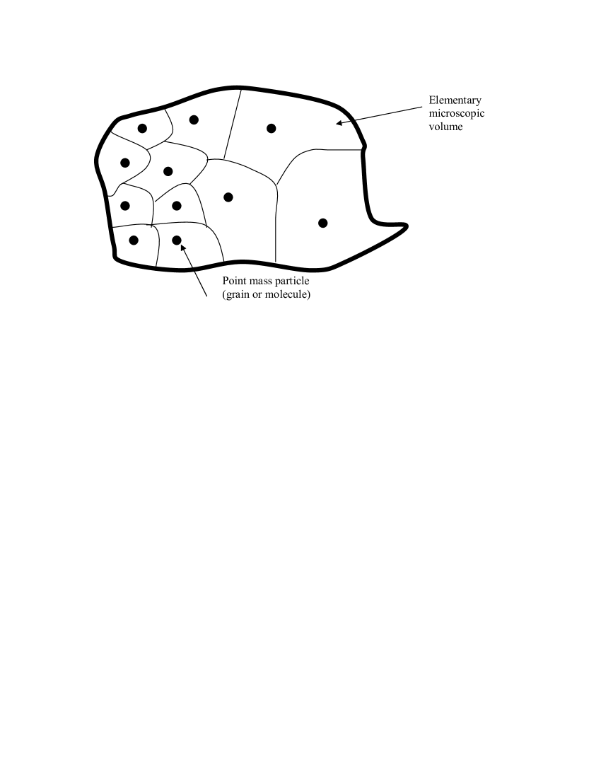
Figure 1: Schematic (essentially, a Voronoi diagram) of microscopic fluid volume distribution around a number of gaseous particles. The elementary microscopic volume is small in regions with a greater number of molecules, and large in regions with fewer molecules. A “volume of fluid” is represented by the physical domain in which the molecules are dispersed.

We note that:

• from a purely mathematical point of view, an “elementary amount of volume” in the second description plays the same role as an “elementary amount of mass” in the first description;

• figure 1 may also be regarded as representing the element termed a “fluid particle” in fluid mechanics, which is a volume domain containing a great number of molecules.

2.3 The two barycentric velocities: volume velocity and mass velocity

Consider the motion of two molecules $P_{1}$ and $P_{2}$ between time $t^{\prime}$ and $t^{\prime\prime}$. At time $t^{\prime}$, the mass of molecule $P_{1}$ is $m_{1}$ and the mass of $P_{2}$ is $m_{2}$. Similarly the microscopic volume associated with $P_{1}$ is $v_{1}$ while that associated with $P_{2}$ is $v_{2}$. Each molecule has a given velocity at each time and at each position (see figure 2), which will be denoted $\xi$.

From a mathematical point of view, two barycentric point systems can be perfectly defined according to the mass of the particles and according to the microscopic volumes associated with the particles. In so doing, we have on one side a system of barycentric points represented by the couples $(m_{i},\xi_{i})$ and on the other side a system represented by the couples $(v_{i},\xi_{i})$. These two barycentric systems lead to two different barycentric velocities (or mean velocities).

More precisely, considering the molecules $P_{1}$ and $P_{2}$, the velocity associated with both molecules, when regarding the mass, is at time $t^{\prime}$ related to $m_{1}\xi_{1}^{\prime}+m_{2}\xi_{2}^{\prime}$ and at time $t^{\prime\prime}$ related to $m_{1}\xi_{1}^{\prime\prime}+m_{2}\xi_{2}^{\prime\prime}$: the mass of each molecule does not change in time. On the other hand, when regarding the volume, the velocity associated with both molecules’ motion is at time $t^{\prime}$ related to $v_{1}^{\prime}\xi_{1}^{\prime}+v_{2}^{\prime}\xi_{2}^{\prime}$ and at time $t^{\prime\prime}$ related to $v_{1}^{\prime\prime}\xi_{1}^{\prime\prime}+v_{2}^{\prime\prime}\xi_{2}^{\prime\prime}$: the microscopic volume does change in time.

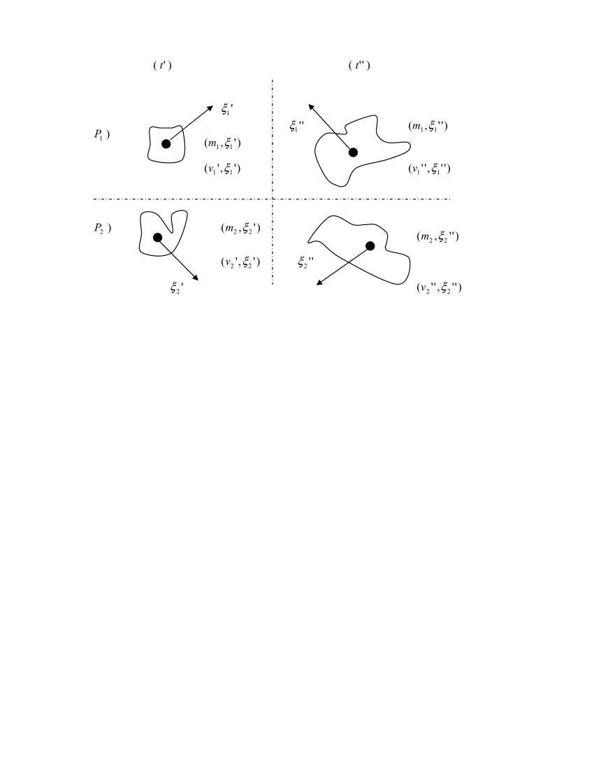
Figure 2: Schematic of “mass barycentric points” and “volume barycentric points”. The elements represented in this figure are to be taken as individual elements from figure 1.

These two barycentric velocities are evidently different, as volume and mass are two different weighting elements. The volume barycentric velocity accounts for the variations of the microscopic volumes in time and space, in addition to the variations of the velocities of the point-mass particles. However, the mass barycentric velocity accounts only for the variations of the velocities of the point-mass particles, since the mass of the molecules is constant.

The two barycentric velocities will only be equivalent if there is a linear relation between mass and microscopic volumes, which would mean a uniform distribution of the particles in the fluid without variation of the global volume occupied the particles.

The barycentric velocities are expressed:

• mass barycentric velocity, $U_{m}$,

  $$\mathrm{Mes}_{m}(\Omega_{m})\cdot U_{m}=\int_{\Omega_{m}}\xi d_{M},$$ (7)

• volume barycentric velocity, $U_{v}$,

  $$\mathrm{Mes}_{v}(\Omega_{v})\cdot U_{v}=\int_{\Omega_{v}}\xi d_{V},$$ (8)

where the integral summations are founded by the measures defined in previous sections, and related to the mass-based and the volume-based representations, respectively.

We note here that the definitions (7) and (8) correspond to what have been termed recently “mass-velocity” and “volume-velocity”, respectively [11, 12]. The distinction between these mean velocities can also be shown from generalized concepts of “centre of mass” in more sophisticated differential geometries in physics [15].

2.4 Hydrodynamic velocities and the equations of fluid mechanics

In contrast to the motion of a solid body, hydrodynamics involves the motion of a “volume of fluid”. The motion of a volume occupied by gaseous molecules is founded on the concept of an element termed a “fluid particle”. Accordingly, the mean velocity of any volume of fluid should be defined by the mean velocity obtained by weighting each microscopic velocity by the respective microscopic volume of fluid.

In other words, and referring again to figure 1, the mean velocity of a fluid particle, which is an element of volume, is not the mean mass-velocity given by the mass-based representation, but the velocity obtained by weighting the microscopic velocities with the microscopic volumes. This is because the mean velocity obtained by using mass as the weighting element corresponds strictly to the velocity of a total amount of mass (the centre of mass), independent of the volume of space occupied and therefore independent of the volume of the fluid particle.

While the velocity of the fluid particle should properly be attributed to the volume-based barycentric velocity, the choice of hydrodynamic velocity is not, however, the sole questionable point in the process of deriving the fluid equations. The main point lies in being consistent in the choice of velocity when performing balances for mass, momentum and energy. This will be addressed below.

2.5 An uncertainty in classical fluid mechanics topology

The two measures described in sections 2.1 and 2.2 are connected to two different ways of performing integrations and balances. In the derivation of the conventional set of fluid mechanics equations, known as the Navier-Stokes equations, a clear distinction has not been made between mass-based integrations and volume-based integrations, and the volume barycentric velocity and the mass barycentric velocity are treated as equivalent.

If $V$ is a control volume of fluid, and $m_{V}$ the total mass contained in $V$, the total amount of any property $Q$ (momentum or energy) carried by the control volume (which is, strictly speaking, the total amount of $Q$ carried by the amount of matter $m_{V}$) is generally given by

$$\int_{\Omega_{m_{V}}}Qd_{M}\ ,$$ (9)

which simply means the summation over all the elementary quantities of $Q$ carried by the elementary point-mass particles contained in the volume $V$.

In classical fluid mechanics, for instance when deriving hydrodynamic equations such as the Navier-Stokes equations, the amount of property $Q$ carried in $V$ is usually taken as

$$\int_{V}\rho Qd_{V}\ ,$$ (10)

where $\rho$ is taken as the fluid mass-density. From a mathematical point of view, the total amount given by expression (9) corresponds to the total amount given by expression (10) if $\rho$ is uniform over the control volume, $V$, i.e. that $d_{M}=\rho d_{V}$. Both expressions are equivalent only if there exists a simple linear relation between the quantity of mass and the quantity of volume.

It is common in fluid mechanics to argue expression (10) through the assumptions that a fluid particle contains a great number of molecules, and that these molecules are uniformly distributed so that $\rho$ can be viewed as being locally constant. However, these classical assumptions cannot be said to be completely fulfilled in some important situations, so a perfect equality between expressions (9) and (10) cannot always be presumed. Balances based on expression (10) seem to be doubtful when (strong) density gradients are present in the fluid, or in sufficiently rarefied gases where the fluid volume must be quite large to incorporate enough molecules.

To ensure equivalence of expressions (10) and (9) from a statistical point of view, we suggest replacing $\rho$ in expression (10) with the mean value, $\left\langle\rho\right\rangle$, of $\rho$ over the fluid particle:

$$\int_{V}\left\langle\rho\right\rangle Qd_{V}\ .$$ (11)

But in this situation, two points need to be emphasised. First, the question of the definition of the mass-density arises, because $\rho$ cannot be simply defined as a limiting value of the mass-to-volume ratio [2]. The mass-density definition introduced in expression (10) is properly defined only when there are sufficient molecules in the fluid particle to smooth out any density fluctuations. Second, if $Q$ is set to be the molecule velocities then expression (10) or (11) embody the equality of “volume barycentric velocity” and “mass barycentric velocity”. That is to say, for a fluid element,

$$\int_{\Omega_{m}}\xi d_{m}=\int_{V}\left\langle\rho\right\rangle\xi d_{V}=\left\langle\rho\right\rangle\int_{\Omega_{v}}\xi d_{V},$$ (12)

then a fluid particle velocity is such that

$$U_{m}=U_{v}.$$ (13)

Obviously, this last equality is mathematically valid only for uniformly distributed molecules, or in the event of equivalence between the two measures described in sections 2.1 and 2.2.

The classical fluid mechanics argument that supports expression (10) is also the local thermodynamic equilibrium assumption in gas dynamics. Assumption of local thermodynamic equilibrium is acceptable when there are no large variations in the thermodynamic parameters in the whole fluid domain concerned. In this case, expression (10) would be valid, as density may be safely considered as locally constant. The gas flow Knudsen number is usually defined as

$$K_{n}=\frac{\lambda_{m}}{\rho}\frac{\delta\rho}{\delta x},$$ (14)

where $\lambda_{m}$ is the molecular mean free path and $x$ a spatial coordinate. Local equilibrium is assumed when $K_{n}\rightarrow 0$, which is the range admitted for validity of the classical Navier-Stokes hydrodynamic equations. The equivalences that we question in this section of the paper are only acceptable in the range $K_{n}\rightarrow 0$. Therefore it remains to investigate how to incorporate local non-uniformity into hydrodynamic models of fluid flows.

2.6 A paradox in the classical continuity equation

Let us consider a mass, $M_{0}$, of some rarefied gas containing a given number, $N_{0}$, of monatomic gaseous particles occupying a volume, $V_{0}$. The particles are uniformly distributed in $V_{0}$. Suppose that at time $t=0$ this gas is placed in a vacuum (with no boundaries and no external force applied). The only forces in the gas are through the interaction potential between particles. We are interested in the time evolution of the mass-density of the fluid.

As the molecules will scatter in all directions, it is expected that the mean mass-velocity will be zero, and the classical continuity equation predicts only a constant mass-density. However, the mass-density of the fluid (i.e. mass divided by volume of the gas) would be expected to decrease in time since the gas volume will grow. Evolution of the mass-density without a mass-velocity is in contradiction to the classical continuity equation.

Anticipating the discussion below and in Appendix A of the difference between number-density and mass-density, another inconsistency in the classical continuity equation is outlined in Appendix B.

3 Kinetic theory and mass-density variations

In this section the problem of local density variations that we have outlined in previous sections is addressed within the framework of the kinetic theory of monatomic gases.

3.1 The distribution function in classical kinetic theory

Consider a physical space with reference to a fixed inertial frame $(X_{1},X_{2},X_{3})$. In classical kinetic theory, $f(t,X,\xi)$, termed “the particle distribution function”, is the probability number-density of particles which, at a given time $t$, have their velocities in the vicinity of the velocity $\xi$, and are located in the vicinity of the fixed reference position $X$. This probability density gives a number of particles at time $t$.

These particles occupy some geometrical domain, $v(t,X)$, in physical space, which is the (local) volume occupied around the fixed position $X$. But the distribution function as it stands does not contain information about how these particles are scattered in $v(t,X)$, or about the measurable value of $v(t,X)$.

We can see that the distribution function, $f(t,X,\xi)$, contains the following information about the molecules at any time, $t$: velocity $\xi$, momentum $M\xi$, energy $M\xi^{2}$. None of the parameters $t$, $X$, or $\xi$ contains information about the real volume occupied by the group of particles. That is to say, macroscopic descriptions derived from these parameters and from $f(t,X,\xi)$ cannot contain information about the volume occupied by the fluid.

The classical assumption about volume in kinetic theory is to consider the space element $d_{X}=d_{X_{1}}d_{X_{2}}d_{X_{3}}$, which defines the vicinity of the reference position $X$ and which is, strictly speaking, a fixed element of space related to the frame $(X_{1},X_{2},X_{3})$. Then it is assumed that the volume occupied by the particles is the fixed element $d_{X}$, and that the molecules are uniformly distributed in this element [2].

Consequently, the classical distribution function, $f(t,X,\xi)$, suffers from the same criticism presented in section 2.5. Nor does the classical conception of a distribution function admit evolution of the volume, $v(t,X)$, occupied by the gaseous molecules in the fixed frame $(X_{1},X_{2},X_{3})$. The current conception of $f(t,X,\xi)$ is suitable for a (locally) uniform dispersion of molecules, and for gases with no large compressibility effects. It cannot correctly treat gases flowing under higher compressibility (or rarefaction) because in these cases the assumption that $d_{X}\equiv v(t,X)$ is doubtful.

3.2 Kinetic theory modified for local density variations

According to our microscopic volume representation of figure 1, a microscopic elementary volume is assigned to each gaseous particle. Therefore, we may consider a distribution function which incorporates the microscopic elementary volume as follows:

$f(t,X,\xi,v)$ is the probability number-density of particles which, at a given time $t$, are located in the vicinity of position $X$, have their velocities in the vicinity of velocity $\xi$, and have an assigned microscopic volume in the vicinity of volume $v$.

It is important to note that what is termed here the “vicinity of reference position $X$” is defined by a fixed element $d_{X}=d_{X_{1}}d_{X_{2}}d_{X_{3}}$ that is related to the fixed reference frame $(X_{1},X_{2},X_{3})$ within which the fluid motion is being investigated. This element must not be confused with the element of volume $v$, which is defined through the real geometrical volume envelope of the space occupied by an ensemble of molecules. In our new $f(t,X,\xi,v)$, $v$ is the measurable positive value of the geometrical microscopic volume, and quite distinct from $X$. The microscopic volume $v$ can vary in an element of volume $d_{X}$: a prescribed number of particles can reduce their volume space or expand it whilst the element $d_{X}$ is kept fixed.

We note that, through our definition of $f(t,X,\xi,v)$, the element $d_{X}$ may or may not contain a great number of particles, and therefore may or may not contain a great number of microscopic volumes of fluid, $v$.

As the origin of any motion is the individual motion of the molecules (and not of the microscopic volumes!), the statistical kinetic equation of the evolution of $f(t,X,\xi,v)$ can be written similarly to the classical Boltzmann kinetic equation, i.e.,

$$\frac{\partial f}{\partial t}+(\xi\cdot\nabla)f+(F\cdot\nabla_{\xi})f+W\frac{\partial f}{\partial v}=\int\int(f^{*}f_{1}^{*}-ff_{1})\sigma\xi_{r}d_{\omega}d_{\xi_{1}},$$ (15)

where $f=f(t,X,\xi,v)$ and $f_{1}=f(t,X,\xi_{1},v_{1})$ refer to post-collision particles, $f^{*}=f(t,X,\xi^{*},v^{*})$ and $f_{1}^{*}=f(t,X,\xi_{1}^{*},v_{1}^{*})$ refer to pre-collision particles, $\xi_{r}=\xi-\xi_{1}$ is the particle relative velocity, $\sigma$ the collision differential cross section, $d_{\omega}$ an element of solid angle, and $\nabla_{\xi}$ denotes the formal operator $\nabla_{\xi}=\partial/\partial\xi_{x}+\partial/\partial\xi_{y}+\partial/\partial\xi_{z}$. We recall that the collision integral (right-hand-side of equation 15), is based on the elementary dynamics of collisions between two point-mass particles, and uses their centre-of-mass.

The new term involving $W$ in equation (15) arises from the introduction of the new variable $v$ into the distribution function. In fact, $W$ may also be written $dv/dt$, and then the supplementary term appears as the variation of $f$ due purely to volume lost to, or gained from, external space. Like the term in $F$, which represents the external body force contribution to the variation of $f$, $W$ represents the contribution of any volume change to the variation of $f$. Obviously, the rate of volume variation, $W$, should not depend on the microscopic parameters, and the variables $t$, $X$, $\xi$ and $v$ are independent. For example, $W$ could be generated by macroscopic pressure gradients. In the following, we will suppose no body force, i.e. $F=0$.

According to our volume representation, the microscopic volume of two different particles involved in a collision is ($v+v_{1}$) after the collision and ($v^{*}+v_{1}^{*}$) before the collision. This microscopic volume will vary in time because the particle repartition is different at each time. During a collision, the microscopic volume carried by the particles is not affected by the dynamics of the interaction. Consequently, the variation of volume during collisions is only due to the variation of the microscopic volumes of both particles in time. As we are considering dilute gases, where the collision time is short compared to other characteristic times, notably the time between two collisions, we can assume that the variation of volume is larger during the relatively long time between two collision than during the short time of the collision itself. As a result, the microscopic volumes can be considered as conserved over the collision time, i.e.

$$v^{*}+v_{1}^{*}=v+v_{1}.$$ (16)

Thus we have, during a collision, a set of four conserved quantities: the microscopic volume, $v$, supplemented by the three usual conserved quantities, i.e. mass, momentum and energy.

3.2.1 Definitions of macroscopic quantities

The local number-density of the molecules within the fixed reference frame (i.e. referring to the element of volume, $d_{X}$) is given by:

$$n(t,X)=\int_{-\infty}^{+\infty}\int_{0}^{+\infty}f(t,X,\xi,v)d_{v}d_{\xi}\ ,$$ (17)

while the local mean value, $\bar{Q}(t,X)$, of any property $Q$ in $d_{X}$ can be defined by:

$$n(t,X)\bar{Q}(t,X)=\int_{-\infty}^{+\infty}\int_{0}^{+\infty}Qf(t,X,\xi,v)d_{v}d_{\xi}\ .$$ (18)

For example, the local mean volume around each particle, $\bar{v}(t,X)$, is defined by:

$$n(t,X)\bar{v}(t,X)=\int_{-\infty}^{+\infty}\int_{0}^{+\infty}vf(t,X,\xi,v)d_{v}d_{\xi}\ .$$ (19)

From this mean value of the microscopic volume, a local mean value of the mass-density in the vicinity of position $X$ can be properly defined through:

$$\bar{\rho}(t,X)=\frac{n(t,X)M}{n(t,X)\bar{v}(t,X)}=\frac{M}{\bar{v}(t,X)}\ ,$$ (20)

where $M$ is the molecular mass. The corresponding specific volume is given by $\bar{v}/{M}$.

We note that $n\bar{v}d_{X}$ is the actual volume of fluid in the vicinity of $X$, containing $nd_{X}$ gaseous molecules. In classical kinetic theory, these $nd_{X}$ molecules are always assumed to occupy, and be uniformly dispersed in, the fixed element of space $d_{X}$. Our new description is evidently different: while the new definitions of mass-density and specific volume represent mean values, and depend on $t$ and $X$, the gaseous molecules need not necessarily be uniformly dispersed in the vicinity of $X$. Moreover, the total volume of fluid around position $X$ is $n\bar{v}d_{X}$, not $d_{X}$.

Appendix A contains more details on distinguishing between $n$ and $\bar{\rho}$.

Two mean velocities can be defined. First, the local mean mass-velocity, $U_{m}(t,X)$, is given through

$$Mn(t,X)U_{m}(t,X)=\int\int M\xi f(t,X,\xi,v)d_{\xi}d_{v}.$$ (21)

A local volume-velocity, $U_{v}(t,X)$, can also be defined by,

$$\bar{v}(t,X)n(t,X)U_{v}(t,X)=\int\int v\xi f(t,X,\xi,v)d_{\xi}d_{v}.$$ (22)

We note that the mean velocities defined through equations (21) and (22) are equivalent to the two velocity definitions pointed out in earlier sections of this paper.

The classical particle peculiar velocity is defined through the mass-velocity, i.e.

$$C=\xi-U_{m}\ .$$ (23)

But another peculiar velocity can also be defined using the volume-velocity $U_{v}$:

$$C^{\prime}=\xi-U_{v}\ .$$ (24)

The peculiar velocity given by equation (23), is usually supposed to define the random motion of the point-mass particles. However, it may be noted in equation (23) that only the macroscopic motion of the centre-of-mass, $U_{m}$, is removed from the point-mass velocities inside the peculiar velocity $C$. Therefore, macroscopic motions due to expansion or compression of the fluid element may still be contained in $C$.

3.2.2 Conservation equations from the modified kinetic equation

We now show the derivation of new macroscopic equations from our kinetic equation (15). This procedure is similar to the classical one: equation (15) is multiplied by the microscopic quantities $v$, $M$, $(M\xi)$, $(M\xi^{2})$ and then the result is integrated over $d_{v}$ and $d_{\xi}$. In this process it should be kept in mind that $t$, $X$, $\xi$, and $v$ are independent variables, while any mean value of a microscopic quantity given through definition (18) depends on $t$ and $X$.

• Conservation of volume. Multiplying equation (15) by the microscopic element $v$, and integrating over $v$ and $\xi$, we obtain,

  $$\int\int v\frac{\partial f}{\partial t}d_{v}d_{\xi}+\int\int v(\xi\cdot\nabla)fd_{v}d_{\xi}+W\int\int v\frac{\partial f}{\partial v}d_{v}d_{\xi}=0,$$ (25)

  where the collision integral term vanishes. Since $t,X,\xi$ and $v$ are independent variables, this equation reduces to

  $$\int\int\frac{\partial vf}{\partial t}d_{v}d_{\xi}+\int\int\nabla\cdot(vf\xi)d_{v}d_{\xi}+W\int\int v\frac{\partial f}{\partial v}d_{v}d_{\xi}=0,$$ (26)

  which can also be written,

  $$\frac{\partial n\bar{v}}{\partial t}+\int\int\nabla\cdot(vfU_{m})d_{v}d_{\xi}+\int\int\nabla\cdot(vfC)d_{v}d_{\xi}+W\int\int v\frac{\partial f}{\partial v}d_{v}d_{\xi}=0.$$ (27)

  Using partial integration and the integrability condition, $\lim_{v\rightarrow+\infty}(vf)=0$, the third integral term in relation (27) gives

  $$W\int\int v\frac{\partial f}{\partial v}d_{v}d_{\xi}=-nW,$$ (28)

  and relation (27) can then be written

  $$\frac{\partial n\bar{v}}{\partial t}+\nabla\cdot[n\bar{v}U_{m}]+\nabla\cdot[\int\int(vCf)d_{v}d_{\xi}]-nW=0.$$ (29)

  Finally, if we denote

  $$\mathbf{J}_{v}=\int\int(vCf)d_{v}d_{\xi},$$ (30)

  then the first macroscopic equation obtained is an evolution equation for the volume, and is written

  $$\frac{\partial n\bar{v}}{\partial t}+\nabla\cdot[n\bar{v}U_{m}]+\nabla\cdot[\mathbf{J}_{v}]=nW.$$ (31)

  The quantity $\mathbf{J}_{v}$ in equation (30) represents a flux of volume due to point-mass particle random motions defined with the peculiar velocity $C$.

  From equations (22) and (23), the local mean volume-velocity of the fluid may be written:

  $$n\bar{v}U_{v}=\int\int vU_{m}f(t,X,\xi,v)d_{\xi}d_{v}+\int\int vCf(t,X,\xi,v)d_{\xi}d_{v}.$$ (32)

  Consequently, the following relation between the volume-velocity and the mass-velocity is deduced:

  $$n\bar{v}U_{v}=n\bar{v}U_{m}+\mathbf{J}_{v}.$$ (33)

• Conservation of mass. Multiplying equation (15) by the molecular mass $M$, and integrating over $v$ and $\xi$, we obtain:

  $$\int\int M\frac{\partial f}{\partial t}d_{v}d_{\xi}+\int\int M(\xi\cdot\nabla)fd_{v}d_{\xi}+W\int\int M\frac{\partial f}{\partial v}d_{v}d_{\xi}=0,$$ (34)

  where the collision integral term vanishes. The third integral term in equation (34) is zero owing to the generalized function character of $f$, i.e. $\lim_{v\rightarrow 0}f=0$ and $\lim_{v\rightarrow+\infty}f=0$. The second macroscopic equation obtained in this case is then:

  $$\frac{\partial Mn}{\partial t}+\nabla\cdot[MnU_{m}]=0,$$ (35)

  which is a typical equation of conservation of mass or, more rigorously, conservation of the number of particles. Combining equation (35) with the volume equation (31) gives

  $$n\left(\frac{\partial\bar{v}}{\partial t}+U_{m}\cdot\nabla\bar{v}\right)+\nabla\cdot[\mathbf{J}_{v}]=nW.$$ (36)

  Using the density $\bar{\rho}=M/\bar{v}$, this can be rewritten:

  $$\left(\frac{\partial\bar{\rho}}{\partial t}+U_{m}\cdot\nabla\bar{\rho}\right)-\frac{\bar{\rho}^{2}}{Mn}\nabla\cdot[\mathbf{J}_{v}]+\frac{\bar{\rho}^{2}}{M}W=0.$$ (37)

• Conservation of momentum. Multiplying equation (15) by $M\xi$, and integrating over $v$ and $\xi$, we obtain

  $$\int\int M\xi\frac{\partial f}{\partial t}d_{v}d_{\xi}+\int\int M\xi(\xi\cdot\nabla)fd_{v}d_{\xi}+W\int\int M\xi\frac{\partial f}{\partial v}d_{v}d_{\xi}=0,$$ (38)

  where the collision integral term vanishes. As $t$ and $\xi$ are independent variables, this equation can be written in the form:

  $$\int\int\frac{\partial Mf\xi}{\partial t}d_{v}d_{\xi}+\int\int\nabla\cdot(Mf\xi_{i}\xi_{j})d_{v}d_{\xi}+W\int\int M\xi\frac{\partial f}{\partial v}d_{v}d_{\xi}=0,$$ (39)

  where $\xi_{i}\xi_{j}$ is the second order tensor constituted by the elements ($\xi_{i}\xi_{j}$). Here also, the third integral term in relation (39) is zero owing to the generalized function character of $f$, i.e. $\lim_{v\rightarrow 0}\xi f=0$ and $\lim_{v\rightarrow+\infty}\xi f=0$. Then, using the definition of peculiar velocity, we obtain the third conservation equation:

  $$\frac{\partial MnU_{m}}{\partial t}+\nabla\cdot\left[MnU_{m}U_{m}\right]+M\nabla\cdot\mathbf{P}=0,$$ (40)

  where $\mathbf{P}\equiv\mathbf{P}_{ij}(t,X)$ is the flux:

  $$\mathbf{P}_{ij}(t,X)=\int\int(C_{i}C_{j})fd_{v}d_{\xi}.$$ (41)

  We note that the conservation equation (40) is a number-density (or mass) based equation and does not contain any volume information, or the density $\bar{\rho}$. Using the mass conservation equation (35), the momentum equation may be written :

  $$n\left(\frac{\partial U_{m}}{\partial t}+U_{m}\cdot\nabla U_{m}\right)+\nabla\cdot\mathbf{P}=0.$$ (42)

• Conservation of energy. Multiplying equation (15) by $\frac{1}{2}M\xi^{2}$ and integrating over $v$ and $\xi$, we obtain

  $$\int\int\frac{1}{2}M\xi^{2}\frac{\partial f}{\partial t}d_{v}d_{\xi}+\int\int\frac{1}{2}M\xi^{2}(\xi\cdot\nabla)fd_{v}d_{\xi}+W\int\int M\xi^{2}\frac{\partial f}{\partial v}d_{v}d_{\xi}=0,$$ (43)

  which, following the independent variable properties, becomes

  $$\int\int\frac{1}{2}M\frac{\partial f\xi^{2}}{\partial t}d_{v}d_{\xi}+\int\int\frac{1}{2}M\nabla\cdot(\xi^{2}f\xi)d_{v}d_{\xi}+W\int\int M\xi^{2}\frac{\partial f}{\partial v}d_{v}d_{\xi}=0.$$ (44)

  Here also, owing to the properties of $f$, i.e. $\lim_{v\rightarrow 0}\xi^{2}f=0$ and $\lim_{v\rightarrow+\infty}\xi^{2}f=0$, the third integral term vanishes. Using the peculiar and the mean velocity definitions, we therefore have

  $$\frac{\partial}{\partial t}\left[\frac{1}{2}MnU_{m}^{2}\right] +\frac{\partial}{\partial t}\left[Mne_{in}\right]+\nabla\cdot\left[\frac{1}{2}MnU_{m}^{2}U_{m}+Mne_{in}U_{m}\right]$$

  $$+\nabla\cdot\left[M\mathbf{P}\cdot U_{m}\right]+\nabla\cdot M\mathbf{q}=0,$$

  where we have introduced the quantity $e_{in}$ that is given through:

  $$n(t,X)e_{in}=\frac{1}{2}\int\int C^{2}fd_{\xi}d_{v},$$ (46)

  and the flux $\mathbf{q}(t,X)$, given by:

  $$\mathbf{q}(t,X)=\frac{1}{2}\int\int C^{2}Cfd_{\xi}d_{v}.$$ (47)

  Equation (• ‣ 3.2.2) is the mean energy evolution equation. Again, this equation is mass-based, and does not involve any volume information. By using the mass conservation equation (35), the energy equation may be rewritten :

  $$n\frac{\partial}{\partial t}\left[\frac{1}{2}U_{m}^{2}+e_{in}\right] +nU_{m}\cdot\nabla\left[\frac{1}{2}U_{m}^{2}+e_{in}\right]$$

  $$+\nabla\cdot\left[\mathbf{P}\cdot U_{m}\right]+\nabla\cdot\mathbf{q}=0.$$

4 A new set of macroscopic conservation equations

The set of macroscopic conservation equations obtained from our modified kinetic equation (15) are:

• equation (36) for the volume;

• equation (35) for the mass;

• equation (42) for the momentum;

• equation (• ‣ 3.2.2) for the energy.

In this set of equations, the mean velocity $U_{m}(t,X)$ is by definition the mass-velocity in each equation; the various fluxes, $\mathbf{J}_{v}(t,X)$, $\mathbf{q}(t,X)$, and $\mathbf{P}(t,X)$ are the fluxes related to the peculiar velocity, $C$, defined in equation (23).

Our new set of macroscopic equations are rewritten below for convenience, using the material derivative $D/Dt\equiv\partial/\partial t+U_{m}\cdot~{}\nabla$

Continuity

$$\frac{Dn}{Dt}=-n\nabla\cdot U_{m},$$ (49)

Mass-density

$$\frac{D\bar{\rho}}{Dt}=\frac{\bar{\rho}^{2}}{M}\left[\frac{1}{n}\nabla\cdot[\mathbf{J}_{v}]-W\right],$$ (50)

Momentum

$$n\frac{DU_{m}}{Dt}=-\nabla\cdot\mathbf{P},$$ (51)

Energy

$$n\frac{D}{Dt}\left[\frac{1}{2}U_{m}^{2}+e_{in}\right]=-\nabla\cdot\left[\mathbf{P}\cdot U_{m}\right]-\nabla\cdot\mathbf{q}\ .$$ (52)

The volume-velocity of the flow is related to the mass-velocity through $n\bar{v}U_{v}=n\bar{v}U_{m}+\mathbf{J}_{v}$ .

5 Discussion

The new set of macroscopic equations, (49)–(52), is a set of four conservation equations instead of the usual three. The main novel aspect of our set of equations is the replacement of the classical continuity equation, which usually involves both the number-density and the mass-density, by two separate equations: a pure conservation equation of mass and an evolution equation for the mass-density.

Although the momentum and energy equations look similar to the classical conservation equations, it should be noted that they are mass-based equations through the number-density $n$, and they do not involve directly the mass-density or the actual volume of fluid. They also refer to a fixed inertial frame. This characteristic matches well the interpretation of equation (51) as Newton’s second law which is, in its correct form, a mass-based law that disregards the actual volume that contains the mass.

In terms of new features introduced by the two new relations in the set of equations, we refer to the difference between an “incompressible flow” and an “incompressible fluid”. Recalling that $\nabla\cdot U_{m}$ is the volume derivative following the velocity $U_{m}$, the continuity equation (49) is interpreted as the number-density variation due to the flow compressibility. On the other hand, fluid compressibility effects, that are due to the variation of the fluid mass-density, are contained in relation (50). The compressibility involved in the new relation (50) can be caused by significant temperature or pressure variations in the fluid as it flows, in contrast to the first form of compressibility effects which are related to the flow speed or acceleration.

The classical fluid mechanics continuity equation combines the mass-density and the number-density in a single equation, which therefore assumes equivalency of compressibility effects arising from the fluid and from the flow speed — although it is well-known experimentally that these two effects are different. Classifying a flow as incompressible or not is difficult in the context of the classical continuum equations [16, 17, 18]. However, in our new model it is clear that a flow without compressibility effects can only be assumed if there are insignificant relative variations of the mass-density (through equation 50) and insignificant volume variation under acceleration, $\nabla\cdot U_{m}=0$ (through equation 49).

The departure of flow solutions of our new set of equations from solutions of the classical equations may be expected in a range of flows that suffer from high fluid compressibility effects, even if the flow itself remains within the conventional incompressible condition (i.e. the flow Mach number less than about $0.3$); examples of such flows include those seen in and around microscale devices [18] and other rarefied gas flow situations.

If there is no mass-density variation then there is no rate of volume variation, i.e. $W=0$, and no flux of volume, i.e. $\mathbf{J}_{v}=0$. In this case, equation (50) disappears and our set of equations reverts to the usual three-equation model in which the mass-density is simply $\bar{\rho}=Mn$. On the other hand, if the mass-velocity, $U_{m}$, is zero then equations (31) and (33) give,

$$\frac{\partial n\bar{v}}{\partial t}+\nabla\cdot[n\bar{v}U_{v}]=nW\ ,$$ (53)

which is thus an equation of expansion (or compression) of the fluid in which $W$ is the term of volume of fluid production. This equation accompanies the energy equation even in situations where the mass-velocity evolution equation (51) can be disregarded. An example of such a situation is the configuration described as paradoxical in section 2.6.

In our modified kinetic equation (15), $W$ appears as the internal rate of change of volume occupied by the gas, and is independent of the microscopic parameters, i.e. $W=dv/dt$. If we assume this rate of change of volume is associated with variations of the macroscopic parameters, such as the fluid temperature and pressure which we denote in this paper as $T^{\prime}$ and $p^{\prime}$, respectively, we can then write the following formal expression,

$$W=\frac{dv}{dt}=\bar{v}\left(\frac{1}{\bar{v}}\frac{\partial v}{\partial T^{\prime}}\right)_{p^{\prime}}\frac{dT^{\prime}}{dt}+\bar{v}\left(\frac{1}{\bar{v}}\frac{\partial v}{\partial p^{\prime}}\right)_{T^{\prime}}\frac{dp^{\prime}}{dt}\ +...\ ,$$ (54)

or

$$W=\bar{v}\alpha\frac{dT^{\prime}}{dt}-\bar{v}\chi\frac{dp^{\prime}}{dt}\ +...\ ,$$ (55)

with compressibility coefficients defined by:

$$\alpha=\left(\frac{1}{\bar{v}}\frac{\partial v}{\partial T^{\prime}}\right)_{p^{\prime}},\hskip 25.00003pt\chi=-\left(\frac{1}{\bar{v}}\frac{\partial v}{\partial p^{\prime}}\right)_{T^{\prime}}\ .$$ (56)

The dimensions of these two coefficients suggest $\alpha\approx 1/T^{\prime}$ and $\chi\approx 1/p^{\prime}$. In this case, these approximations represent simple equations to describe the variations of the volume around gaseous particles as a function of the fluid macroscopic parameters; they should not be taken as a derivation of an equation of state. This is because equations (54) and (55) concern variations of the “microscopic volume” around each particle, while a thermodynamic equation of state is correctly applied only to a “macroscopic volume” of fluid — and requires equilibrium conditions.

Using the above approximation for $W$, the mass-density equation (50) can be rewritten:

$$\frac{D\bar{\rho}}{Dt}=\frac{\bar{\rho}^{2}}{Mn}\nabla\cdot[\mathbf{J}_{v}]-\bar{\rho}\left(\alpha\frac{dT^{\prime}}{dt}-\chi\frac{dp^{\prime}}{dt}\right)\ .$$ (57)

In this equation, the left-hand-side derivative is the material derivative that involves $U_{m}$ while on the right-hand-side is a total derivative which does not always equal the material derivative. For example, the total derivative, $d\ /dt$, may be expressed using velocity $U_{v}$ rather than the mass velocity $U_{m}$, i.e.

$$\frac{d}{dt}=\frac{\partial}{\partial t}+U_{m}\cdot\nabla+\frac{1}{n\bar{v}}\mathbf{J}_{v}\cdot\nabla\ .$$ (58)

Now, equation (57) enables us to solve in outline the problem posed in section 2.6. We admit zero mass velocity in this flow configuration, so equation (57) is re-written

$$\frac{1}{\bar{\rho}}\frac{\partial\bar{\rho}}{\partial t}=\frac{\bar{\rho}}{Mn}\nabla\cdot[\mathbf{J}_{v}]-\left(\alpha\frac{dT^{\prime}}{dt}-\chi\frac{dp^{\prime}}{dt}\right)\ .$$ (59)

As we are only concerned with the variation in time, we may assume an approximately uniform evolution of the fluid domain, i.e $\nabla\cdot[\mathbf{J}_{v}]=0$ (i.e. the flux of volume depends only on time, not space). Then the solution of this problem is determined through

$$\frac{1}{\bar{\rho}}\frac{\partial\bar{\rho}}{\partial t}=-\left(\alpha\frac{dT^{\prime}}{dt}-\chi\frac{dp^{\prime}}{dt}\right)\ .$$ (60)

This solution is independent of the number-density, $n$ (which is connected to the fixed reference frame of the observer), so the solution of equation (60) is independent of the reference frame. As the compressibility coefficients do not depend explicitly on time, but only on the gas properties such as temperature and pressure, then the solution of equation (60) can be written:

$$\bar{\rho}=\bar{\rho}_{0}\exp\left\{\alpha(T^{\prime}-T^{\prime}_{0})-\chi(p^{\prime}-p^{\prime}_{0})\right\}\ ,$$ (61)

with $\bar{\rho}_{0}\equiv\bar{\rho}_{0}(X)$, $p^{\prime}_{0}\equiv p^{\prime}_{0}(X)$ and $T^{\prime}_{0}\equiv T^{\prime}_{0}(X)$ the initial values of mass-density, pressure and temperature of the gas. As a result, equation (61) gives the evolution of the mass-density with the temperature and the pressure — although this does not affect the assumption of mass conservation embodied in equation (49).

Equation (60) is not completely new; it, or an approximate form, is usually assumed in fluid mechanics for flows presenting density variation effects. The originality of our model is that this equation is actually embodied in the kinetic equation (15). This equation is therefore not a simple phenomenological relation, as usually presented, but is contained within the full set of conservation equations. Equation (60) describes the local mean value of the mass-density even when the classical assumption of real local uniformity does not hold.

6 Conclusions

In this article we have suggested there may be inconsistencies in the classical treatment of the “mass of fluid” and the “volume of fluid” descriptions. These inconsistencies appear to become important (a) if significant relative variations in density arise in the fluid, and/or (b) in flows in which the local equilibrium assumption does not hold. Two different representations of fluids have been outlined, and a volume-based kinetic approach has been introduced through a slightly modified version of the Boltzmann kinetic equation.

The set of macroscopic equations derived from our modified kinetic equation has a fundamental departure from the classical description of fluid mechanics: an evolution equation purely of the mass-density is added to the set of three conservation equations (for number-density, momentum and energy). While conservation of mass is embodied in an equation involving only the particle number-density, mass-density evolution is embodied in a separate conservation equation which invokes a flux of volume and incorporates parameters that can generate fluid volume variation (such as temperature or pressure variations). Our new model, therefore distinguishes between compressibility effects arising from the “fluid compressibility” and from the “flow compressibility”.

The nature of the velocity appearing in the classical Navier-Stokes set of equations has recently been questioned [12]. It has been suggested, although without rigorous proof, that in the set of fluid mechanics equations the velocity to be used when writing the Newton viscosity law should be the volume-velocity. In the present article we have shown that, from the kinetic theory point of view, mass-velocity and volume-velocity can be properly defined: mass-velocity gives only the velocity of the centre-of-mass of a fluid element, while volume velocity accounts for expansion or compression of the fluid element.

In classical kinetic theory, the pressure tensor and heat flux are systematically attributed to the fluxes $\mathbf{P}_{ij}(t,X)$ and $\mathbf{q}(t,X)$ appearing in the conservation of momentum and energy equations, and these fluxes are founded on the peculiar velocity. But in the new volume-based kinetic approach introduced in this paper, two different peculiar velocities can be defined. Therefore further investigations are required in order to connect the real pressure tensor, heat flux, and internal energy of the fluid to the various fluxes appearing in the set of conservation equations. We address this issue in a complementary paper, so that a complete set of hydrodynamic equations is derived.

Appendix A Further comments on the definitions of number-density and mass-density

A.1 Preliminaries

Let us consider a fixed inertial reference frame, $\mathfrak{R}_{G}$, with reference to the coordinate elements $(X_{1},X_{2},X_{3})$. In this fixed reference we investigate the motion of a cubic volume element of fluid. We suppose that our cubic element of fluid is always attached to a moving reference frame, $\mathfrak{R}_{F}$, with coordinate elements $(F_{1},F_{2},F_{3})$. Moreover, our cubic element of fluid is determined at any time by the three base vectors of the reference frame $\mathfrak{R}_{F}$.

For simplicity we assume that initially both reference frames coincide, i.e., initially the three base vectors of both frames $\mathfrak{R}_{G}$ and $\mathfrak{R}_{F}$ are the same. Regarding the fixed frame $\mathfrak{R}_{G}$, the second frame representing our element of fluid can have the following types of motions: translation, rotation (according to three Eulerian angles), and expansion or compression.

An element of volume in the fixed reference frame is denoted by $d_{X}=d_{X_{1}}d_{X_{2}}d_{X_{3}}$ while an element of volume in the frame representing the cubic element of fluid is $d_{F}=d_{F_{1}}d_{F_{2}}d_{F_{3}}$. The element of volume $d_{X}$ and $d_{F}$ may be formally linked by relation

$$d_{X}=Jd_{F},$$ (62)

where $J$ is the absolute value of the Jacobian determinant of the transformation of $\mathfrak{R}_{G}$ into $\mathfrak{R}_{F}$. If $\mathfrak{R}_{F}$ is undergoing only translations or rotations in the fixed reference $\mathfrak{R}_{G}$, then $J=1$ as rotation and translation conserve volumes. Otherwise, if compression or expansion occurs then we have $J\neq 1$.

A.2 The number density, $n$, and the mass-density, $\bar{\rho}$

In our new kinetic approach introduced in this paper, $f(t,X,\xi,v)$ is a probability number density in the phase space $(X,\xi,v)$. This means the number of particles within an element of volume of this phase space, $d_{X}d_{\xi}d_{v}$, is $f(t,X,\xi,v)d_{X}d_{\xi}d_{v}$. The number of particles around a position, $X$, may be denoted $n(t,X)d_{X}$ :

$$n(t,X)d_{X}=\int_{-\infty}^{+\infty}\int_{0}^{+\infty}f(t,X,\xi,v)d_{\xi}d_{v}.$$ (63)

The total number of gaseous particles in the whole space referenced by the fixed frame $\mathfrak{R}_{G}$ is

$$N=\int n(t,X)d_{X}\ .$$ (64)

Accordingly, $n(t,X)$ appears as a “number-density” referring to the fixed reference frame $(X_{1},X_{2},X_{3})$. It is a number of particles divided by the fixed element of volume $d_{X}$.

Because of expansion or compression of the reference frame $(F_{1},F_{2},F_{3})$ during motion, we cannot presume a correspondence between the element of volume $d_{X}$ and the element of volume $d_{F}$ which gives the actual volume of the fluid. Therefore, the correct number-density referring to the real volume occupied by the fluid is not directly given by $n$ but may be different by the dilatation or compression coefficient $J$.

As the mean value of the microscopic volume of fluid around the particles, $\bar{v}$, is defined through

$$n(t,X)\bar{v}(t,X)=\int_{-\infty}^{+\infty}\int_{0}^{+\infty}vf(t,X,\xi,v)d_{v}d_{\xi}\ ,$$ (65)

it is found, using equation (63), that the volume occupied by the fluid at reference position $X$ is given by $(nd_{X})\bar{v}$, i.e. the total number of microscopic volumes of fluid (or number of particles) multiplied by the mean value of these microscopic volumes, $\bar{v}$. This volume of fluid contains $nd_{X}$ gaseous molecules. Therefore, when we refer to the actual volume of the fluid, the “number-density” is

$$\frac{nd_{X}}{n\bar{v}d_{X}}=\frac{1}{\bar{v}}\ .$$ (66)

The fluid density (or mass-density) in its physical meaning at position $X$ is then

$$\bar{\rho}=\frac{Mnd_{X}}{n\bar{v}d_{X}}=\frac{M}{\bar{v}}\ .$$ (67)

A.3 The classical kinetic theory view of density

In classical kinetic theory, molecules are assumed to always occupy, and be uniformly dispersed in, the element of space $d_{X}$ without a clear distinction between the actual volume occupied by the gaseous molecules and the physical space connected to the fixed inertial reference frame. Chapman & Cowling [2] state that: “…the mass contained by $d_{X}$ will be proportional only to its volume, and will not depend on its shape…Similarly, the number of molecules in $d_{X}$ …is proportional to $d_{X}$. It will be denoted by $nd_{X}$; $n$ is called the number-density of molecules.”

In others words, $nd_{X}$ is the number of particles in the volume element $d_{X}$ which itself is regarded as the volume of the fluid. Therefore, in this description expansion or compression of the volume element $d_{F}$ in the fixed reference $(X_{1},X_{2},X_{3})$ is disregarded.

According to this classical view, the number-density referring to the element of volume $d_{X}$ is written

$$\frac{nd_{X}}{d_{X}}=n\ ,$$ (68)

while the volume of fluid around each particle is given by

$$\frac{d_{X}}{nd_{X}}=\frac{1}{n}\ .$$ (69)

We see that the classical description imposes directly a unit volume of fluid given by the inverse of the number density $n$. From our equation (66), the unit volume of fluid is $\bar{v}$, which refers to the actual volume of the fluid, $d_{F}$. The classical unit volume, $1/n$, refers to the volume element $d_{X}$ of the fixed inertial reference frame. These quantities may therefore differ by a compression/dilatation coefficient $J$.

If the particles are uniformly distributed, i.e. no mass density variation in the fluid, then $nd_{X}$ is the number of particles always occupying uniformly the volume $d_{X}$. In this case, the mean microscopic volume, $\bar{v}$, around each particle is given by the volume $d_{X}$ divided by the number of particles $nd_{X}$,

$$\bar{v}=\frac{d_{X}}{nd_{X}}=\frac{1}{n}.$$ (70)

Consequently, only in this particular situation does the definition of the mass-density, equation (67), become

$$\bar{\rho}=\frac{M}{\bar{v}}=Mn\ .$$ (71)

Generally, however, $Mn$ is different from $\bar{\rho}$. The density quantity $Mn$ may be regarded as the density of a similar fluid under similar conditions although with compression and expansion motions removed; the actual density of the fluid is given by $\bar{\rho}$. The product $n\bar{v}$ behaves like a compression/dilatation coefficient, which depends on time and position.

Finally, the distinction between the actual element of volume of fluid and the simple element of volume taken in the fixed inertial reference frame raises a question of consistency in the definition of the pressure tensor from kinetic theory. The pressure tensor definition invokes a volume element of fluid for which the classical conceptual frame does not make a distinction between the fixed element, $d_{X}$, and the element of volume of fluid, $d_{F}$. The real element of fluid should therefore be decoupled from the fixed frame of the observer.

Appendix B The Euler form of the continuity equation

Here we consider incompressible flows, by which we mean only $\nabla\cdot U_{m}=0$. We suppose, however, that variations of density, and then variations of the volume, of a fluid element can exist; for example, through variations of temperature in time and space.

Let us follow a fixed amount of mass, $M_{f}$, of fluid, occupying at time $t_{0}$ a volume $V_{0}$, and occupying at time $t$ the volume $V$. In classical fluid mechanics, if we denote $\rho\equiv\rho(t,X)$ the density of the fluid, then we should have

$$M_{f}=\int_{V_{0}}\rho_{0}d_{V_{0}}=\int_{V}\rho d_{V}\ .$$ (72)

A change of variables can be applied so that

$$\int_{V_{0}}\rho_{0}d_{V_{0}}=\int_{V_{0}}\rho Jd_{V_{0}}\ ,$$ (73)

where, as in equation (62), $J$ is due to the application transforming $V_{0}$ into $V$. Equation (73) may be applied at $t=t_{0}$, in which case $J(t=t_{0})=J_{0}=1$. So equation (73) can be written

$$\int_{V_{0}}[J_{0}\rho_{0}-J\rho]d_{V_{0}}=0\ .$$ (74)

As $M_{f}$ is an arbitrary amount of mass, and $V_{0}$ an arbitrary volume, equation (74) becomes

$$[J_{0}\rho_{0}-J\rho]=0\ ,$$ (75)

so we can write the following:

$$\frac{D(J\rho)}{Dt}=0\ ,$$ (76)

for any time $t$. In equation (76) the derivative is a material (convective) derivative because we are explicitly moving with the mass, as we impose $M_{f}$ to be constant. This equation, due to Euler, is known as the material form of the continuity equation [19]. We note that in our case $J$ depends on time $t$: at $t=t_{0}$, $J=1$, but nothing is stated about the derivative of $J$ (i.e., nothing imposes $DJ/Dt=0$ for $t=t_{0})$.

The local form of the conventional continuity equation (with $\nabla\cdot U_{m}=0$) is

$$\frac{D\rho}{Dt}=0\ .$$ (77)

Therefore, a contradiction appears between the material form of the continuity equation (76) and the common fluid mechanics expression (77) because $J$ depends on time — but these two expressions should be the same as they are expressing the same physical law.

Using our description of density from Appendix A, the density of the fluid which should be used in equations (72)–(76) is $\rho=\bar{\rho}=M/\bar{v}$, where the expansion/compression coefficient $J$ is $n\bar{v}$. So, replacing these elements in equation (76), we find

$$\frac{D(Mn)}{Dt}=0\ ,$$ (78)

which is the correct local form of the mass continuity equation: the contradiction existing between the Euler equation (76) and the classical local form of the continuity equation disappears in our description in which the density is $\bar{\rho}$, equation (67), and the local form of the continuity equation is equation (78). The Euler equation (76) and equation (78) are therefore entirely equivalent in our description.

The density of the fluid, $\bar{\rho}$, which varies according to changes in the properties of the fluid, satisfies the Euler form of the continuity equation; the quantity $Mn$ behaves like a reference density, retracing the conservation of mass from a reference frame in which any change in the properties of the fluid is observed. Our reference amount of mass, $M_{f}$, is simply always constant.

References

- [1] P. L. Bhatnagar, E. P. Gross, M. Krook, A model for collision processes in gases: 1. small amplitude processes in charged and neutral one-component systems, Physical Review 94 (3) (1954) 511–525.
- [2] S. Chapman, T. Cowling, The Mathematical Theory of Non-Uniform Gases, 3rd Edition, Cambridge Mathematical Library, 1970.
- [3] C. Cercignani, Mathematical Methods in Kinetic Theory, 2nd Edition, Plenum Press, New York, 1990.
- [4] H. Grad, On the kinetic theory of rarefied gases, Communications on Pure and Applied Mathematics 2 (4) (1949) 331–407.
- [5] D. A. Lockerby, J. M. Reese, M. A. Gallis, The usefulness of higher-order constitutive relations for describing the Knudsen layer, Physics of Fluids 17 (2005) 100609.
- [6] J. M. Reese, M. A. Gallis, D. A. Lockerby, New directions in fluid dynamics: non-equilibrium aerodynamic and microsystem flows, Philosophical Transactions of the Royal Society of London A 361 (2003) 2967–2988.
- [7] T. Koga, A proposal for fundamental equations of dynamics of gases under high stress, Journal of Chemical Physics 22 (10) (1954) 1633–1646.
- [8] H. Struchtrup, Macroscopic Transport Equations for Rarefied Gas Flows: Approximation Methods in Kinetic Theory, Springer, 2005.
- [9] R. S. Myong, A generalized hydrodynamic computational model for rarefied and microscale diatomic gas flows, Journal of Computational Physics 195 (2) (2004) 655–676.
- [10] S. Jin, M. Slemrod, Regularization of the Burnett equations via relaxation, Journal of Statistical Physics 103 (5-6) (2001) 1009–1033.
- [11] H. Brenner, Kinematics of volume transport, Physica A 349 (1-2) (2005) 11–59.
- [12] H. Brenner, Navier-Stokes revisited, Physica A 349 (1-2) (2005) 60–132.
- [13] H. C. Ottinger, Beyond Equilibrium Thermodynamics, Wiley-Interscience, 2005.
- [14] A. Bardow, H. C. Ottinger, Consequences of the Brenner modification to the Navier-Stokes equations for dynamic light scattering, submitted to Journal of Chemical Physics.
- [15] M. Pavsic, Clifford space as the arena for physics, Foundations of Physics 33 (9) (2003) 1277–1306.
- [16] A. H. Shapiro, The Dynamics and Thermodynamics of Compressible Fluid Flow, John Wiley, 1953.
- [17] G. L. Morini, M. Lorenzini, S. Colin, S. Geoffroy, Experimental investigation of the compressibility effects on the friction factor of gas flows in microtubes, 4th ASME International Conference on Nanochannels, Minichannels and Microchannels, 2006.
- [18] M. Gad-el-Hak, The fluid mechanics of microdevices, ASME Journal of Fluids Engineering 121 (1999) 5–33.
- [19] L. E. Malvern, Introduction to the Mechanics of a Continuous Medium, Prentice-Hall, Inc., 1969.