Signature of ray chaos in quasibound wave functions for a stadium-shaped dielectric cavity

Abstract

Light emission from a dielectric cavity with a stadium shape is studied in both ray and wave models. For a passive cavity mode with low loss, a remarkable correspondence is found between the phase space representation of a quasibound wave function and its counterpart distribution in the ray model. This result provides additional and more direct evidence for good ray-wave correspondence in low-loss modes previously observed at the level of far-field emission pattern comparisons.

Directional lasing emission is one of the most highlighted features of two-dimensional microcavity lasers ARC . In interpreting the appearance of emission directionality and its dependence on cavity shape, a ray dynamical model has proven useful ARC ; Hentschel01 ; Schwefel04 ; Fukushima04 ; SB.Lee06 ; Lebental06 . In the standard version of the ray model, Frenel’s law is applied to describe the light emission process from a cavity without its application being fully justified; Frenel’s law is usually derived when a plane wave is scattered at a planer dielectric interface. For a cavity shape obeying integrable ray dynamics, one can approximately make a connection between the ray picture based on Frenel’s law and wave solutions in the short-wavelength limit by using the Eikonal method Tureci03 . Besides, even for a nonintegrable cavity, one can associate its stable ray trajectory (if it exists) to a class of wave solutions by the Gaussian-optical method Tureci02 . For a fully chaotic cavity, however, one lacks a method to relate ray trajectories with wave solutions. Whereas establishing ray-wave (or classical-quantum) correspondence in closed chaotic systems has been very matured in the field of quantum chaos QC , it is still an ongoing issue to make such a correspondence in “open” systems Open_sys , one of which being dielectric microcavities.

In this paper, we present numerical evidence showing that for a fully chaotic cavity, there is significant correspondence between ray dynamics and solutions of the Helmholtz equation, although we currently lack justification for applying the ray model to a fully chaotic cavity. We consider a stadium-shaped cavity as shown in the inset of Fig. 1, whose internal ray dynamics is known to become fully chaotic Bunimovich . Stadium-shaped cavities have actually been fabricated using materials such as semiconductors Fukushima04 and polymers Lebental06 , and stable lasing has been experimentally confirmed in both materials. In particular, for polymer cavities (refractive index $n\approx 1.5$), the ray model predicts highly directional light emission, which can be associated with the unstable manifolds of a short periodic trajectory of the stadium cavity Schwefel04 ; Shinohara06 . This highly directional emission has been experimentally observed, and systematic agreement between experimental far-field patterns and those obtained from the ray model has been reported in Ref. Lebental06 . Moreover, in recent work, we employed a nonlinear lasing model based on the Maxwell-Bloch equations SB to numerically simulate the lasing of polymer stadium cavities and successfully obtained a highly directional far-field emission pattern that agrees with the ray model’s prediction Shinohara06 . The analysis of the passive cavity modes relevant for lasing revealed that each of the low-loss (or high-$Q$) modes exhibits the far-field emission pattern closely corresponding to the ray model’s results. The present work provides more direct and clearer evidence for this ray-wave correspondence by showing that the phase space representation of wave functions reproduces the ray model’s distribution formed by the stretching and folding mechanisms of ray chaos.

As a method to relate a wave function with ray dynamics, the Husimi phase space distribution is often used SB.Lee06 ; Tureci05 ; Hentschel03 ; SY.Lee . To accord with the definition of the phase space for the ray model, where only the collisions with the boundary with outgoing momentum are taken into account, it is appropriate to decompose a wave function into radially incoming and outgoing components and then project the latter onto the phase space. Such decomposition has been implemented by using the expansion in terms of the Hankel functions Tureci05 , which is, however, only suited for a cavity shape slightly deformed from a circle. Hence, here we introduce a different phase space distribution that can be formally related with the ray model’s distribution and directly calculated from the wave function and its normal derivative at the boundary.

First, we introduce a ray model incorporating Frenel’s law. In what follows, we fix the refractive indices inside and outside the cavity as $n_{in}=1.5$ and $n_{out}=1.0$, respectively, and restrict our attention to transverse magnetic (TM) polarization. Inside the cavity, we regard the dynamics of a ray as a point particle that moves freely except for bounces at the cavity boundary satisfying the law of reflection. We assign a ray trajectory a variable $\varepsilon(t)$ representing intensity at time $t$, where $t$ is measured by trajectory length in real space. Due to the collision with the boundary at time $t$, the ray intensity changes as $\varepsilon(t^{+})={\cal R}\,\varepsilon(t^{-})$, where $t^{-}$ and $t^{+}$ are the times just before and after the collision and ${\cal R}$ is the Fresnel reflection coefficient for TM polarization Hecht : ${\cal R}=[\sin(\phi-\phi_{t})/\sin(\phi+\phi_{t})]^{2},$ where $\phi$ and $\phi_{t}$ are incident and transmission angles related by Snell’s law $n_{in}\sin\phi=n_{out}\sin\phi_{t}$. Since we do not consider any pumping effect, $\varepsilon(t)$ is a monotonically decreasing function.

Ray dynamics can be reduced to a two-dimensional area-preserving mapping on the phase space defined by the Birkhoff coordinates $(s,p)$, where $s$ is the curvilinear coordinate along the cavity boundary and $p=\sin\phi$ is the tangential momentum along the boundary. The intensity leakage at the cavity boundary creates an “open window” in the momentum space: Whenever a ray trajectory comes into region $|p|<p_{c}=n_{out}/n_{in}$, it loses intensity by amount ${\cal T}\,e$, where ${\cal T}$ is the transmission coefficient, i.e., ${\cal T}=1-{\cal R}$, that can be expressed by sole variable $p$.

We assume that initially rays are distributed uniformly over the phase space having identical intensities. To study the statistical properties of the ray model, we focus upon a time-independent distribution $P(s,p)$ that describes intensity flux at the cavity boundary. The usefulness of studying this distribution has been demonstrated in Refs. Shinohara06 ; SY.Lee ; Ryu06 . Below we define this distribution for the ray model and later derive the corresponding distribution for the wave model.

We denote the light intensity inside the cavity as ${\cal E}(t)=\sum_{j}\varepsilon_{j}(t)$, where the sum is taken over the ray ensembles. Its time evolution can be written as

$$\frac{d{\cal E}}{dt}=-\int_{0}^{S}ds\int_{-p_{c}}^{p_{c}}dp\,{\cal T}(p)\,{\cal F}(s,p,t),$$ (1)

where ${\cal F}(s,p,t)$ represents intensity flux at the cavity boundary and $S$ the total boundary length.

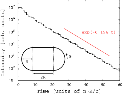
Figure 1: (Color online) Exponential decay of light intensity in the ray model, where the time is measured in the unit of $n_{in}R/c$. Inset shows geometry of the stadium-shaped cavity.

It has been numerically shown that ${\cal E}(t)$ exhibits exponential decay behavior for stadium cavities Ryu06 . Performing a numerical simulation with $10^{7}$ ray ensembles, we obtain ${\cal E}(t)$ as shown in Fig. 1. We can estimate the exponential decay rate as $\gamma_{r}\approx 0.194\times c/(n_{in}R)$, where $c$ is the light speed outside the cavity and $R$ the radius of the circular part of the stadium cavity. Exponential decay ${\cal E}(t)={\cal E}(0)\,e^{-\gamma_{r}t}$ can be derived from Eq. (1) by assuming that ${\cal F}(s,p,t)$ can be factorized as ${\cal F}(s,p,t)=F(s,p)\,{\cal E}(t)$ SY.Lee , where the decay rate $\gamma_{r}$ can be expressed as

$$\gamma_{r}=\int_{0}^{S}ds\int_{-p_{c}}^{p_{c}}dp\,P(s,p).$$ (2)

Here, we put $P(s,p)={\cal T}(p)F(s,p)$ for convenience. $P(s,p)$ describes how the rays’ intensities are transmitted outside the cavity and becomes important when trying to understand the relation between emission directionality and the phase space structures of ray dynamics Schwefel04 ; SY.Lee ; Shinohara06 . Figure 2 (a) shows a numerically obtained distribution $P(s,p)$. As explained in detail in Refs. Schwefel04 ; Shinohara06 , the structure of the high-intensity regions of $P(s,p)$ can be well fitted by the unstable manifolds of a pair of unstable four-bounce periodic trajectories; one is located just above critical line $p=p_{c}$ and the other just below $p=-p_{c}$.

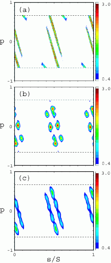
Figure 2: (Color) (a) Intensity flux distribution $P(s,p)$ for the ray model. (b) Phase space distribution $H(s,p)$ of a wave function for a low-loss mode with $kR=100.00024-0.12667i$. (c) The average of $H(s,p)$ of the 21 lowest-loss modes. Dashed lines represent critical lines $p=\pm p_{c}$. Note that $P(s,p)$ and $H(s,p)$ are normalized to $\gamma_{r}$ as in Eq.(2)

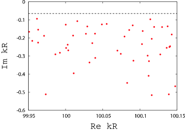
Figure 3: (Color online) Distribution of resonances for $k_{r}R\approx 100$. Prediction from the ray model is plotted in a dashed line.

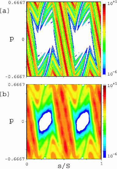
Figure 4: (Color) (a) Log₁₀ plot of the intensity flux distribution $P(s,p)$ shown in Fig. 2 (a). (b) Log₁₀ plot of the averaged distribution $H(s,p)$ shown in Fig. 2 (c). Only region $|p|\leq p_{c}$ is shown.

Let us next treat the light field by the Maxwell equations. For a two-dimensional cavity, the $z$-component of the TM electric field is written as $E_{z}(x,y,t)=\mbox{Re}[\psi(x,y)\,e^{-i\omega t}]$, where $\psi(x,y)$ satisfies the Helmholtz equation $[\nabla_{xy}^{2}+n^{2}(x,y)\,k^{2}]\,\psi=0$ and $\omega=ck$. For a dielectric cavity, the eigensolutions of the Helmholtz equation become quasibound states (or resonances) characterized by complex wave numbers $k=k_{r}+ik_{i}$ with $k_{i}<0$. Wave numbers $k$ and wave functions $\psi$ can be numerically obtained by the boundary element method Wiersig03 . In Fig. 3, we plot the distribution of the resonances for $k_{r}R\approx 100$. For the wave description, the light intensity decay rate $\gamma_{w}$ is written as $\gamma_{w}=2c|k_{i}|$. Equating $\gamma_{w}$ with $\gamma_{r}$ evaluated in the ray simulation, one obtains the ray model’s estimate of the $k_{i}R$ value, i.e., $k_{i}R=-0.194/(2n_{in})\approx-0.0647$, which turns out in this case to give an upperbound of the $k_{i}R$ values as shown in Fig. 3. It is an interesting problem to establish a precise correspondence between $\gamma_{r}$ and $\gamma_{w}$ by a semiclassical argument, which however we will not pursue here.

Next, we derive a distribution for the wave description that corresponds to $P(s,p)$, formulating the intensity decay process as in the ray model. The light intensity of the cavity is written as ${\cal E}=\int\int_{\cal D}dxdy\frac{1}{2}(\epsilon\vec{E}^{2}+\mu\vec{H}^{2})$, where ${\cal D}$ represents the area of the cavity and $\epsilon$ and $\mu$ are electric permittivity and magnetic permeability, respectively. The time evolution of ${\cal E}$ can be written as

$$\frac{d{\cal E}}{dt}=-\int_{0}^{S}ds\,{\cal S}(s,t),$$ (3)

where ${\cal S}(s,t)$ is the component of the Poynting vector normal to the cavity boundary, i.e., ${\cal S}(s,t)=cE_{z}(-\nu_{x}H_{y}+\nu_{y}H_{x})$, where $\vec{\nu}$ is a unit vector normal to the cavity boundary. In the TM case, $H_{x}$ and $H_{y}$ are determined from $E_{z}$ through $\partial E_{z}/\partial y=-(\mu/c)(\partial H_{x}/\partial t)$ and $\partial E_{z}/\partial x=(\mu/c)(\partial H_{y}/\partial t)$. ${\cal S}(s,t)$ contains terms rapidly oscillating in time with frequency $2ck_{r}$. We smooth out this rapid oscillation by $\bar{\cal S\,}(s,t)=\frac{1}{T}\int_{t}^{t+T}d\tau{\cal S}(s,\tau)$ with $T=2\pi/(ck_{r})$. Assuming $k_{r}\gg|k_{i}|$, which is valid in the low-loss and short-wavelength limit, one obtains

$$\bar{\cal S\,}(s,t)=\frac{ce^{2ck_{i}t}}{2\mu k_{r}}\mbox{Im}\left[\psi^{*}(s)\partial_{v}\psi(s)\right],$$ (4)

where $\partial_{\nu}=\vec{\nu}\cdot\nabla$. Moreover, we coarse-grain spatial variations smaller than the wavelength by applying Gaussian smoothing as follows:

$$\bar{\bar{{\cal S}\,}}(s,t)=\frac{1}{\sigma\sqrt{\pi}}\sum_{n=-\infty}^{\infty}\int_{0}^{S}ds^{\prime}\,e^{\left\{-\frac{(s^{\prime}-s-nS)^{2}}{\sigma^{2}}\right\}}\bar{\cal S\,}(s^{\prime},t),$$ (5)

where $\sigma=\sqrt{S/(2n_{in}k_{r}R)}$. Plugging the right-hand side of Eq. (4) into $\bar{\cal S\,}$ in Eq. (5), we obtain the following expression for $\bar{\bar{{\cal S\,}}}(s,t)$:

$$\bar{\bar{{\cal S\,}}}(s,t)=\frac{ce^{2ck_{i}t}}{2\mu k_{r}}\frac{1}{2\pi}\int_{-\infty}^{\infty}dp\,H(s,p).$$ (6)

Here, $H(s,p)$ is a phase space representation of $\psi^{*}(s)\,\partial_{\nu}\psi(s)$ similar to the Husimi distribution, defined by

$$H(s,p)=\mbox{Im}\left[h_{\psi}^{*}(s,p)\,h_{\partial_{\nu}\psi}(s,p)\right],$$ (7)

where

$$h_{f}(s,p)=\int_{0}^{S}ds^{\prime}\,G^{*}(s^{\prime};s,p)f(s^{\prime})$$ (8)

and $G(s^{\prime};s,p)$ is a coherent state for a one-dimensional periodic system:

$$G(s^{\prime};s,p)=\frac{1}{\sqrt{\sigma\sqrt{\pi}}}\sum_{n=-\infty}^{\infty}e^{\left\{-\frac{(s^{\prime}-s-nS)^{2}}{2\sigma^{2}}+ip(s^{\prime}-s-nS)\right\}}.$$ (9)

Comparing Eqs. (1) and (3) with ${\cal S}(s,t)$ being replaced with $\bar{\bar{{\cal S\,}}}(s,t)$, one finds that $H(s,p)$ is the distribution that should be compared with $P(s,p)$.

Calculating $H(s,p)$ for all the cavity modes shown in Fig. 3, we confirmed that for a low-loss mode, $H(s,p)$ is predominantly supported on the high-intensity regions of $P(s,p)$. We show a typical example in Fig. 2 (b), where we note that to compare with $P(s,p)$ shown in Fig. 2 (a), the momentum is rescaled as $p/(n_{in}k_{r}R)\to p$ and $H(s,p)$ is normalized to $\gamma_{r}$: $\int\int dsdpH(s,p)=\gamma_{r}$. We plot the average of $H(s,p)$ of the 21 lowest-loss modes (i.e., those with $k_{i}R>-0.20$) in Fig. 2 (c), which not only proves that the localization on the high-intensity regions of $P(s,p)$ is a common feature of low-loss modes, but also shows that the correspondence with $P(s,p)$ becomes better by this averaging. The correspondence between $P(s,p)$ and the averaged $H(s,p)$ can be further revealed by plotting these distributions in logarithm scale as shown in Fig. 4: The log₁₀ plot of $P(s,p)$ reveals the structure of low-intensity regions, which can be associated with the long-term behavior of the unstable manifolds of the four-bounce periodic trajectories located near the critical lines. From Fig. 4 (b), one can confirm that the averaged $H(s,p)$ reproduces even the low-intensity regions of $P(s,p)$.

The ray-wave correspondence in low-loss modes provides a natural explanation why experimental far-field patterns agree with the ray model’s prediction. In experiments, lasing often occurs in multi-mode, so that a lasing state can be considered as a “superposition” of multiple low-loss modes. The observation that better ray-wave correspondence is obtained after the averaging over low-loss modes suggests that such a superposition might enhance the ray-wave correspondence.

We thank M. Lebental for showing us unpublished data on ray model simulations and S. Sunada for discussions. The work at ATR was supported in part by the National Institute of Information and Communications Technology of Japan.

References

- (1) J. U. Nöckel and A. D. Stone, in Optical Processes in Microcavities, edited by R. K. Chang and A. J. Campillo (World Scientific, Singapore, 1996); J. U. Nöckel and A. D. Stone, Nature (London) 385, 45 (1997); C. Gmachl, F. Capasso, E. E. Narimanov, J. U. Nöckel, A. D. Stone, J. Faist, D. L. Sivco, and A. Y. Cho, Science 98, 1556 (1998).
- (2) M. Hentschel and M. Vojta, Opt. Lett. 26, 1764 (2001).
- (3) H. G. L. Schwefel, N. B. Rex, H. E. Türeci, R. K. Chang, A. D. Stone, T. B. Messaoud, and J. Zyss, J. Opt. Soc. Am. B 21, 923 (2004).
- (4) T. Fukushima and T. Harayama, IEEE J. Quantum Electron. 10, 1039 (2004).
- (5) S.-B. Lee, J.-B. Shim, S.W. Kim, J. Yang, S. Moon, J.-H. Lee, H.-W. Lee, and K. An, arXiv:physics/0603249; J.-B. Shim, H.-W. Lee, S.-B. Lee, J. Yang, S.M. Moon, J.-H. Lee, K. An, S.W. Kim, arXiv:physics/0603221.
- (6) M. Lebental, J. S. Lauret, R. Hierle, and J. Zyss, Appl. Phys. Lett. 88, 031108 (2006); M. Lebental, J. S. Lauret, J. Zyss, C. Schmit, and E. Bogomolny, arXiv:physics/0609009.
- (7) H. E. Türeci, Ph.D thesis, Yale University, 2003.
- (8) H. E. Türeci, H. G. L. Schwefel, A. D. Stone, and E. E. Narimanov, Optics Express 10, 752 (2002).
- (9) M. C. Gutzwiller, Chaos in Classical and Quantum Mechanics (Springer, Berlin, 1990); H. J. Stockmann, Quantum Chaos: An Introduction (Cambridge University Press, Cambridge, England, 1999).
- (10) J. P. Keating, M. Novaes, S. D. Prado, and M. Sieber, Phys. Rev. Lett. 97, 150406 (2006); S. Nonnenmacher and M. Rubin, arXiv:nlin.CD/0608069.
- (11) L. A. Bunimovich, Commun. Math. Phys. 65, 295 (1977).
- (12) S. Shinohara, T. Harayama, H. E. Türeci, and A. D. Stone, Phys. Rev. A 74, 033820 (2006).
- (13) T. Harayama, P. Davis, and K. S. Ikeda, Phys. Rev. Lett. 90, 063901 (2003); T. Harayama, S. Sunada, and K. S. Ikeda, Phys. Rev. A 72, 013803 (2005).
- (14) M. Hentschel, H. Schomerus, and R. Schubert, Europhys. Lett. 62, 636 (2003).
- (15) H. E. Türeci, H. G. L. Schwefel, Ph. Jacquod, and A. D. Stone, Prog. Opt. 47, 75 (2005).
- (16) S.-Y. Lee, S. Rim, J.-W. Ryu, T.-Y. Kwon, M. Choi, and C.-M. Kim, Phys. Rev. Lett. 93, 164102 (2004); S.-Y. Lee, J.-W. Ryu, T.-Y. Kwon, S. Rim, and C.-M. Kim, Phys. Rev. A 72, 061801(R) (2005).
- (17) E. Hecht, Optics (Addison-Wesley, Reading, MA, 1987).
- (18) J.-W. Ryu, S.-Y. Lee, C.-M. Kim, and Y.-J. Park, Phys. Rev. E 73, 036207 (2006).
- (19) J. Wiersig, J. Opt. A, Pure Appl. Opt. 5, 53 (2003).