On the strategy frequency problem in batch Minority Games

Abstract

Ergodic stationary states of Minority Games with $S$ strategies per agent can be characterised in terms of the asymptotic probabilities $\phi_{a}$ with which an agent uses $a$ of his strategies. We propose here a simple and general method to calculate these quantities in batch canonical and grand-canonical models. Known analytic theories are easily recovered as limiting cases and, as a further application, the strategy frequency problem for the batch grand-canonical Minority Game with $S=2$ is solved. The generalization of these ideas to multi-asset models is also presented. Though similarly based on response function techniques, our approach is alternative to the one recently employed by Shayeghi and Coolen for canonical batch Minority Games with arbitrary number of strategies.

1 Introduction

The mathematical theory of Minority Games (MGs) with $2$ strategies per agent, particularly for what concerns their ergodic behaviour, largely rests on the possibility of separating the contribution to macroscopic quantities coming from “frozen” agents from that of “fickle” ones [1, 2]. Frozen agents are those who use just one of their strategies asymptotically, whereas fickle agents flip between their strategies even in the steady state. That these two groups have different impact on the physical properties of MGs is clear if one thinks that frozen agents are insensitive to small perturbations and thus they do not contribute to the susceptibility of the system. More generally, when agents dispose of $S>2$ strategies each, the relevant quantity to calculate is the probability with which an agent uses $a$ of his strategies ($a\in\{0,1,\ldots,S\}$), knowledge of which provides all interesting physical observables. On the technical level, this is a rather complicated problem that has been tackled only recently in [3] for the canonical $S$-strategy batch MG. Here we propose an alternative method to derive the desired statistics in generic canonical or grand-canonical [4] settings with $S$ strategies per agent. This approach has the advantage of being simpler from a mathematical viewpoint and, as we will show, easily exportable to other versions of the MG. As in [3], we resort to path-integral techniques, allowing for a description of the multi-agent dynamics in terms of the behavior of a single, effective agent subject to a non-trivially correlated noise. The central idea of the method we propose is to exchange the integration over the effective noise for one over frequencies using a simple invertible mapping from one set of variables to the other and the transformation law of probability distributions. We show that available theories are easily recovered in known cases and, as a further application, solve the strategy frequency problem for the grand-canonical MG with $S=2$. Since a similar issue arises in the context of multi-asset MGs [5], we also discuss the (straightforward though heavier from a notational viewpoint) generalisation of this idea to models in which traders may invest in $K\geq 2$ assets.

Since path integrals are by now a somewhat standard technique to deal with MGs, we shall skip mathematical details and focus our analysis on the resulting effective dynamics and specifically on the strategy frequency problem. Moreover, we shall reduce the discussion of the economic meaning of the model to the minimum. The interested reader will find extensive accounts in [1, 2, 6].

2 Model definitions, TTI steady states and the strategy frequency problem

We consider a market for a single asset with $N$ agents, labeled by $i\in\{1,\ldots,N\}\equiv\mathbb{Z}_{N}$. At each time step $\ell$, agents receive an information pattern $\mu(\ell)\in\mathbb{Z}_{P}$ chosen randomly and independently with uniform probability and, based on this, they formulate their bids (represented simply by a variable encoding the agent’s decision, e.g. to buy or sell the asset). The most interesting phenomenology is obtained when $P$ scales linearly with $N$; their ratio, denoted as $\alpha=P/N$, is the model’s main control parameter. Every agent $i$ disposes of $S$ trading strategies $\{a_{is}^{\mu}\}_{s\in\mathbb{Z}_{S}}$, each prescribing a binary action $a^{\mu}_{is}\in\{-1,1\}$, drawn randomly and uniformly, and independently for each strategy $s$ and pattern $\mu$. The performance of every strategy is monitored by a score function $U_{is}(\ell)$ which is updated by

$$U_{is}(\ell+1)-U_{is}(\ell)=-a_{is}^{\mu(\ell)}A(\ell)-\epsilon_{is}/\sqrt{N}$$ (1)

Here, $\epsilon_{is}$ are real constants representing positive or negative incentives for the agents to trade, with a factor $\sqrt{N}$ ensuring a non-trivial behavior in the limit $N\to\infty$. $A(\ell)$ is instead the (normalized) excess demand at time $\ell$,

$$A(\ell)=\frac{1}{\sqrt{N}}\sum_{i\in\mathbb{Z}_{N}}b_{i}(\ell)$$ (2)

where $b_{i}(\ell)$ is the bid formulated by agent $i$ at time $\ell$. If we denote by $s_{i}(\ell)$ the strategy chosen by $i$ at time $\ell$, then the bid submitted by $i$ is given by

$$b_{i}(\ell)=\sum_{s\in\mathbb{Z}_{S}}n_{is}(\ell)a_{is}^{\mu(\ell)}\delta_{s,s_{i}(\ell)}$$ (3)

The terms $a_{is}^{\mu(\ell)}\delta_{s,s_{i}(\ell)}$ impose that the agent performs the action dictated by his selected strategy. The term $n_{is}(\ell)\equiv F[U_{is}(\ell)]$, with $F:\mathbb{R}\to\mathcal{I}$, denotes a filter linked to the score of the selected strategies. We focus our attention on two cases:

• Taking $F$ to be the Heaviside function, one has $\mathcal{I}=\{0,1\}$ so that the filter consists in either submitting ($n_{is_{i}(\ell)}=1$ for $U_{is_{i}(\ell)}>0$) or not submitting ($n_{is_{i}(\ell)}=0$ for $U_{is_{i}(\ell)}<0$) the bid. This version of the game is usually called grand-canonical MG [4].

• If $F\equiv 1$, the filter is absent and agents are forced to play no matter how bad their scores perform. This corresponds to the standard canonical MG.

It remains to describe how $s_{i}(\ell)$ is chosen. We assume generically that at each time step agent $i$ employs a rule described by a function $g_{i}$, namely

$$s_{i}(\ell)=g_{i}\left[\{U_{is}(\ell)\}_{s\in\mathbb{Z}_{S}}\right]$$ (4)

For example, the standard MG with $S=2$ corresponds to $s_{i}(\ell)={\rm arg~{}}\max_{s\in\mathbb{Z}_{S}}U_{is}(\ell)$. (This generalises easily to the case of traders with decision noise [7].) At this stage, we assume that the $g_{i}$’s are chosen randomly and independently across agents (from some distribution) and introduce the density of the mappings $\{g_{i}\}_{i\in\mathbb{Z}_{N}}$ as

$$W[g]=\frac{1}{N}\sum_{i\in\mathbb{Z}_{N}}\delta_{(F)}(g-g_{i})$$ (5)

with $\delta_{(F)}(\cdots)$ a functional Dirac delta. A similar random choice is made for incentives (albeit in general with a different and uncorrelated distribution) and we define their density as

$$w({\mbox{\boldmath$\epsilon$}})=\frac{1}{N}\sum_{i\in\mathbb{Z}_{N}}\prod_{s\in\mathbb{Z}_{S}}\delta\left(\epsilon_{s}-\epsilon_{is}\right)$$ (6)

with ${\mbox{\boldmath$\epsilon$}}=\{\epsilon_{s}\}_{s\in\mathbb{Z}_{S}}$.

We will work out the ‘batch’ version of the model, which is obtained by averaging (1) over information patterns [8]. After a time re-scaling (we denote the re-scaled time as $t$), one obtains the ‘batch’ dynamics

$$U_{is}(t+1)-U_{is}(t)=\theta_{i}(t)-\alpha\epsilon_{is}-\frac{1}{\sqrt{N}}\sum_{\mu\in\mathbb{Z}_{P}}a_{is}^{\mu}\frac{1}{\sqrt{N}}\sum_{s\in\mathbb{Z}_{S}}\sum_{j\in\mathbb{Z}_{N}}n_{js}(t)a_{js}^{\mu}\delta_{s,s_{j}(t)}$$ (7)

where $\theta_{i}(t)$ is a (small) external perturbation added for later use. In dynamical studies, one is interested in the average bid autocorrelation function

$$C(t,t^{\prime})=\frac{1}{N}\sum_{i\in\mathbb{Z}_{N}}\left[\left\langle b_{i}(t)b_{i}(t^{\prime})\right\rangle\right]_{dis}$$ (8)

and in the average response function

$$G(t,t^{\prime})=\frac{1}{N}\sum_{i\in\mathbb{Z}_{N}}\left[\frac{\partial\left\langle b_{i}(t)\right\rangle}{\partial\theta_{i}(t^{\prime})}\right]_{dis}$$ (9)

where $\left\langle\cdots\right\rangle$ and $[\cdots]_{dis}$ denote, respectively, averages over paths and disorder. Assuming that $\theta_{i}(t)=\theta(t)$ for all $i$, in the limit $N\to\infty$ the multi-agent dynamics (7) can be described in terms of a self-consistent stochastic process for a single, effective agent endowed with $S$ strategies, characterized by score functions $U_{s}(t)$, “spin” variable $s(t)=g\left[\{U_{s}(t)\}_{s\in\mathbb{Z}_{S}}\right]$ and filter $n_{s}(t)=F[U_{s}(t)]$. This process can be derived by introducing a generating function of the original dynamics and averaging over disorder [9]. Details of the calculation follow closely those of similar models reported in the literature (see e.g. [2]). The effective dynamics ultimately reads

$$U_{s}(t+1) = U_{s}(t)+\theta(t)-\alpha\epsilon_{s}-\alpha\sum_{t^{\prime}\leq t}[{\mbox{\boldmath{1}{I}}}+G]^{-1}(t,t^{\prime})n_{s}(t^{\prime})\delta_{s(t^{\prime}),s}+\eta_{s}(t)\,,$$ (10)

where $\eta_{s}(t)$ is a coloured Gaussian noise with first moments given by

$$\left\langle\eta_{s}(t)\right\rangle_{\star}=0$$ (11)

$$\left\langle\eta_{s}(t)\eta_{s^{\prime}}(t^{\prime})\right\rangle_{\star}=\delta_{s,s^{\prime}}\alpha[({\mbox{\boldmath{1}{I}}}+G)^{-1}C({\mbox{\boldmath{1}{I}}}+G^{\dagger})^{-1}](t,t^{\prime})$$ (12)

and where

$$C(t,t^{\prime})=\sum_{s\in\mathbb{Z}_{S}}\int d{\mbox{\boldmath$\epsilon$}}\,w({\mbox{\boldmath$\epsilon$}})\int dg\,W[g]\,\left\langle n_{s}(t)n_{s}(t^{\prime})\delta_{s,s(t)}\delta_{s,s(t^{\prime})}\right\rangle_{\star}$$ (13)

$$G(t,t^{\prime})=\sum_{s\in\mathbb{Z}_{S}}\int d{\mbox{\boldmath$\epsilon$}}\,w({\mbox{\boldmath$\epsilon$}})\int dg\,W[g]\,\frac{\delta\left\langle n_{s}(t)\delta_{s,s(t)}\right\rangle_{\star}}{\delta\theta(t^{\prime})}$$ (14)

are the correlation and response functions, respectively.

We focus henceforth on ergodic steady-state properties, and more precisely on time-translation invariant (TTI) solutions of (13) and (14). To do so we require that (a) two-time quantities are Toeplitz-type matrices, i.e. $C(t,t^{\prime})=C(t-t^{\prime})$, $G(t,t^{\prime})=G(t-t^{\prime})$, and that (b) there is no anomalous integrated response, i.e. $\chi:=\lim_{\tau\to\infty}\sum_{t\leq\tau}G(t)<\infty$. We denote time-averages as

$$\overline{x}=\lim_{\tau\to\infty}\frac{1}{\tau}\sum_{t=1}^{\tau}x(t)$$ (15)

Rewriting the scores as $U_{s}(t)=tu_{s}(t)$ and averaging over time we obtain

$$u_{s}=\overline{\theta}+\overline{\eta}_{s}-\alpha\epsilon_{s}-m\sum_{n\in\mathcal{I}}nf_{ns}$$ (16)

where we have defined $m\equiv\frac{\alpha}{1+\chi}$, $u_{s}=\lim_{\tau\to\infty}u_{s}(\tau)$ and

$$f_{ns}=\lim_{\tau\to\infty}\frac{1}{\tau}\sum_{t=0}^{\tau-1}\delta_{n,n_{s}(t)}\delta_{s(t),s}$$ (17)

In what follows, we set $\overline{\theta}=0$ (the response function can be equally evaluated by a derivative with respect to the effective noise $\overline{\eta}_{s}$). Note that (16) describes an ensemble of processes, since in the stationary limit the noise variables $\{\overline{\eta}_{s}\}_{s\in\mathbb{Z}_{S}}$ are Gaussian distributed, viz.

$$P(\overline{{\mbox{\boldmath$\eta$}}})=\prod_{s\in\mathbb{Z}_{S}}\frac{1}{\sqrt{2\pi\varsigma^{2}}}\exp\left[-\frac{\overline{\eta}^{2}_{s}}{2\varsigma^{2}}\right]\,,\quad\varsigma^{2}=\frac{\alpha c}{(1+\chi)^{2}}$$ (18)

where the persistent autocorrelation $c=\lim_{\tau\to\infty}(1/\tau)\sum_{t\leq\tau}C(t)$ and susceptibility $\chi$ can be computed through

$$c=\sum_{s\in\mathbb{Z}_{S}}\sum_{n,n^{\prime}\in\mathcal{I}}n\,n^{\prime}\int d{\mbox{\boldmath$\epsilon$}}\,w({\mbox{\boldmath$\epsilon$}})\int dg\,W[g]\,\left\langle f_{ns}f_{n^{\prime}s}\right\rangle_{\star}$$ (19)

$$\chi=\frac{1}{\varsigma^{2}}\sum_{s\in\mathbb{Z}_{S}}\sum_{n\in\mathcal{I}}n\int d{\mbox{\boldmath$\epsilon$}}\,w({\mbox{\boldmath$\epsilon$}})\int dg\,W[g]\,\left\langle\overline{\eta}_{s}f_{ns}\right\rangle_{\star}$$ (20)

The coefficients $\{f_{ns}\}_{n\in\mathcal{I},s\in\mathbb{Z}_{S}}$ have the meaning of frequencies. Indeed, $f_{ns}$ is the frequency of use of strategy $s$ when the filter takes the value $n$. Clearly,

$$\sum_{n\in\mathcal{I}}\sum_{s\in\mathbb{Z}_{S}}f_{ns}=1$$ (21)

Equation (16) is the staring point of our analysis.The problem consists specifically in calculating the statistics of the frequency variables. For the sake of clarity, we shall now work out the mathematical details of the strategy frequency problem in the case recently addressed in the literature, namely that of the canonical MG ($F\equiv 1$) with $S$ strategies [3]. Following sections will address more complicated versions of the model.

3 Canonical batch Minority Game with $S$ strategies

Recalling that for canonical models $n=1$, in this section we simplify the notation and write $f_{s}$ in place of $f_{ns}$. Furthermore, in order to make direct contact with the case discussed in [3], we assume that $\epsilon_{s}=0$ for each $s\in\mathbb{Z}_{S}$ and that the density $W[g]$ is a $\delta$-distribution with

$$s(t)=g[\{U_{s}(t)\}]={\rm arg\,max}_{s\in\mathbb{Z}_{S}}U_{s}(t)$$ (22)

The stationary state equations now greatly simplify: for each $s$ we have

$$u_{s} = \overline{\eta}_{s}-mf_{s}\,,\quad m\equiv\frac{\alpha}{1+\chi}\,,\quad\sum_{s\in\mathbb{Z}_{S}}f_{s}=1$$ (23)

where $f_{s}$ is the frequency of use of strategy $s$. The statistics of the frequencies can be evaluated as follows. Consider the case in which the effective agent uses a subset of strategies $\mathcal{A}\subseteq\mathbb{Z}_{S}$ ($\mathcal{A}\neq\emptyset$). Due to the rule (22) this automatically implies that

$$u_{s} = u\,,\quad{\rm for~{}}s\in\mathcal{A}\,,$$ (24)

$$u_{s} < u\,,\quad{\rm for~{}}s\not\in\mathcal{A}$$ (25)

with $u$ a generic value of the score velocity. In turn, one has that $\sum_{s\in\mathcal{A}}f_{s}=1$, the rest of the frequencies being identically zero. Let us split the Gaussian variables in two groups:

$$\overline{\eta}_{s}=\cases{x_{s}&for $s\in\mathcal{A}$\\ y_{s}&for $s\not\in\mathcal{A}$}$$ (26)

We have

$$x_{s}\equiv x_{s}\left(u,\{f_{s}\}_{s\in\mathcal{A}}\right)\,, \quad{\rm for~{}}s\in\mathcal{A}$$ (27)

$$y_{s}<u\,, \quad{\rm for~{}}s\not\in\mathcal{A}$$ (28)

where $x_{s}\left(u,\{f_{s}\}_{s\in\mathcal{A}}\right)\equiv u+mf_{s}$ The family of equations (27) defines an invertible mapping $\{x_{s}\}_{s\in\mathcal{A}}\to(u,\{f_{s}\}_{s\in\mathcal{A}})$ whose Jacobian is given by

$$\left|\frac{\partial\{x_{s}\}_{s\in\mathcal{A}}}{\partial(u,\{f_{s}\}_{s\in\mathcal{A}})}\right|=|\mathcal{A}|m^{|\mathcal{A}|-1}$$ (29)

where $|\mathcal{A}|$ is the cardinality of $\mathcal{A}$. We now have all the information required to compute the frequency distribution in this case. By simply invoking the transformation law of probability distribution for the $\mathbf{x}$-variables, i.e.

$$P(\textbf{x})d\textbf{x}=\varrho(u,\textbf{f})du\,d\textbf{f}$$ (30)

from whence

$$\varrho(u,\textbf{f})\equiv P[\textbf{x}(u,\textbf{f})]\left|\frac{\partial\textbf{x}}{\partial(u,\textbf{f})}\right|\,,\quad\textbf{f}=\{f_{s}\}_{s\in\mathbb{Z}_{S}}$$ (31)

and the restriction over the distribution of the y-variables, we have that the contribution to the frequency distribution of the subset $\mathcal{A}$ of strategies with score $u$, denoted $\varrho_{\mathcal{A}}(u,\textbf{f})$, reads

$$\varrho_{\mathcal{A}}(u,\textbf{f})=|\mathcal{A}|m^{|\mathcal{A}|-1}\delta\left(\sum_{s\in\mathcal{A}}f_{s}-1\right)\left[\prod_{s\not\in\mathcal{A}}\delta_{f_{s},0}\right]P[\textbf{x}(u,\{f_{s}\}_{s\in\mathcal{A}})]\left\langle\prod_{s\not\in\mathcal{A}}\Theta\left(u-y_{s}\right)\right\rangle_{\textbf{y}}$$ (32)

where we have used the fact that the noise distribution factorises, i.e. $P({\mbox{\boldmath$\eta$}})=P(\textbf{x})P(\textbf{y})$ and emphasised through the Dirac $\delta$-distributions the constraints over the frequencies. $\left\langle\cdots\right\rangle_{\textbf{y}}$ denotes instead average over the statistics of the y-variables.

Now the whole frequency distribution is simply given by the sum over all possible partitions of $\mathbb{Z}_{S}$ (empty set not included). Thus the average over the initial set of Gaussian variables is converted to average over the frequency distribution:

$$\left\langle(\cdots)\right\rangle_{\star}=\sum_{\mathcal{A}\subseteq\mathbb{Z}_{S}|\mathcal{A}\neq\emptyset}\int du\,d\textbf{f}\,\varrho_{\mathcal{A}}(u,\textbf{f})\,(\cdots)$$ (33)

A further simplification is allowed here if one restricts the attention to subsets with $|\mathcal{A}|=a$ by considering the frequency distribution of $a$ strategies. By standard application of combinatorics, one has

$$\varrho_{a}(u,\textbf{f})=\frac{S!}{(a-1)!(S-a)!}\,m^{a-1}\delta\left(\sum_{s\in\mathbb{Z}_{a}}f_{s}-1\right)\left[\prod_{s\not\in\mathbb{Z}_{a}}\delta_{f_{s},0}\right]P[\textbf{x}(u,\{f_{s}\}_{s\in\mathbb{Z}_{a}})]$$

$$\times\left\langle\prod_{s\not\in\mathbb{Z}_{a}}\Theta\left(u-y_{s}\right)\right\rangle_{\textbf{y}}$$ (34)

and, in turn,

$$\left\langle(\cdots)\right\rangle_{\star}=\sum_{a\in\mathbb{Z}_{S}}\left\langle(\cdots)_{a}\right\rangle_{\star} = \sum_{a\in\mathbb{Z}_{S}}\int du\int d\textbf{f}\,\varrho_{a}(u,\textbf{f})(\cdots)_{1}$$ (35)

Now if we denote by $\phi_{a}$ the fraction of agents using $a$ strategies, then

$$\phi_{a}=\int du\,d\textbf{f}\,\varrho_{a}(u,\textbf{f})$$ (36)

It easy to see that for $\phi_{1}$ and $\phi_{2}$ we obtain

$$\phi_{1} = S\int\frac{du}{\sqrt{2\pi\varsigma^{2}}}e^{-\frac{(u+m)^{2}}{2\varsigma^{2}}}\left[\frac{1}{2}+\frac{1}{2}{\rm Erf}\left(\frac{u}{\sqrt{2\varsigma^{2}}}\right)\right]^{S-1}$$ (37)

$$\phi_{2} = S(S-1)m\int_{0}^{1}\frac{df}{\sqrt{2\pi\varsigma^{2}}}\int\frac{du}{\sqrt{2\pi\varsigma^{2}}}e^{-\frac{(u+mf)^{2}}{2\varsigma^{2}}}e^{-\frac{[u+m(1-f)]^{2}}{2\varsigma^{2}}}\left[\frac{1}{2}+\frac{1}{2}{\rm Erf}\left(\frac{u}{\sqrt{2\varsigma^{2}}}\right)\right]^{S-2}$$ (38)

which, after some straightforward manipulations, is identified with the corresponding formulas of [3].

4 Grand-canonical MG with one asset and $S$ strategies

We now turn our attention to the grand-canonical version of the MG with $S>1$ strategies strategies per agent. This is obtained by taking, in addition to the rules used in the previous section, $n_{is}(t)=F[\{U_{is}(t)\}]=\Theta[U_{is}(t)]$ instead of $F\equiv 1$. Now the stationary state equations read, for each $s\in\mathbb{Z}_{S}$,

$$u_{s} = \overline{\eta}_{s}-\alpha\epsilon_{s}-mf_{s}\,,\quad m\equiv\frac{\alpha}{1+\chi}\,,\quad\varphi+\sum_{s\in\mathbb{Z}_{S}}f_{s}=1$$ (39)

where we set $f_{1s}=f_{s}$ and denoted by $\varphi$ the probability that the agent is inactive, that is the probability that $n=0$. In this case the value of the frequencies for $n=0$ do not enter in the relevant equations which determine the quantities of interest of the model. We proceed to calculate the statistics of the frequencies $\{f_{s}\}_{s\in\mathbb{Z}_{S}}$ and to relate all quantities to such statistics. As before, let $\mathcal{A}\subseteq\mathbb{Z}_{S}$ be a subset of strategies being used, so that

$$u=u_{s}\,,\quad\forall s\in\mathcal{A}$$ (40)

$$u>u_{s}\,,\quad\forall s\not\in\mathcal{A}$$ (41)

Now we must distinguish three cases: if $u>0$, the agent is always active, that is $\varphi=0$; if instead $u=0$, the agent is sometimes inactive, that is $\varphi>0$; finally if $u<0$ then $\varphi=1$ and the agent never invests.

1. Case $u>0$. Here the analysis follows closely the one performed for the canonical $S$-strategy MG. The agent is in the market and $f_{s}\in[0,1]$ represents the frequency of the strategy $s$ being used. This implies that $f_{s}\neq 0$, $\forall s\in\mathcal{A}$ and $f_{s}=0$ $\forall s\not\in\mathcal{A}$ with $\sum_{s\in\mathcal{A}}f_{s}=1$. We then split the stationary equations (39) into two parts and write

   $$x_{s}=x^{+}_{s}\left(u,\{f_{s}\}_{s\in\mathcal{A}}\right)\,, \quad\forall s\in\mathcal{A}$$ (42)

   $$y_{s}<u+\alpha\epsilon_{s}\,, \quad\forall s\not\in\mathcal{A}$$ (43)

   where we have defined the functions

   $$x^{+}_{s}\left(u,\{f_{s}\}_{s\in\mathcal{A}}\right)\equiv u+mf_{s}+\alpha\epsilon_{s}$$ (44)

   and, as before, denoted as $\{x_{s}\}$ the Gaussian variables in the subset $\mathcal{A}$ and as $\{y_{s}\}$ those not belonging to this subset. The set of equations (42) defines an invertible mapping $\{x_{s}\}_{s\in\mathcal{A}}\to(u,\{f_{s}\}_{s\in\mathcal{A}})$ whose Jacobian reads

   $$\left|\frac{\partial\{x^{+}_{s}\}_{s\in\mathcal{A}}}{\partial(u,\{f_{s}\}_{s\in\mathcal{A}})}\right|=|\mathcal{A}|m^{|\mathcal{A}|-1}\,,$$ (45)

   with $|\mathcal{A}|$ the cardinality of the subset $\mathcal{A}$. Proceeding as in the previous section, that is using the transformation law of probability distributions, we find that the contribution to the the frequency distribution of the subset $\mathcal{A}$ of strategies, denoted $\varrho_{\mathcal{A}}(u>0,\textbf{f})$, reads

   $$\varrho_{\mathcal{A}}(u>0,\textbf{f})=|\mathcal{A}|m^{|\mathcal{A}|-1}\Theta(u)\delta\left(\sum_{s\in\mathcal{A}}f_{s}-1\right)\left[\prod_{s\not\in\mathcal{A}}\delta_{f_{s},0}\right]P[\textbf{x}^{+}(u,\{f_{s}\}_{s\in\mathcal{A}})]$$

   $$\times\left\langle\prod_{s\not\in\mathcal{A}}\Theta\left(u+\alpha\epsilon_{s}-y_{s}\right)\right\rangle_{\textbf{y}}$$ (46)

2. Case $u=0$. We now must take into account the fact that $\sum_{s\in\mathcal{A}}f_{s}+\varphi=1$ with $0\leq\varphi\leq 1$. The stationary equations become

   $$x_{s} = x^{0}_{s}\left(\{f_{s}\}_{s\in\mathcal{A}}\right)\,,\quad\forall s\in\mathcal{A}$$ (47)

   $$y_{s} < \alpha\epsilon_{s}\,,\quad\forall s\not\in\mathcal{A}$$ (48)

   with

   $$x^{0}_{s}\left(\{f_{s}\}_{s\in\mathcal{A}}\right)\equiv mf_{s}+\alpha\epsilon_{s}\,.$$ (49)

   The set of equations $x_{s}=x_{s}^{0}(\{f_{s}\}_{s\in\mathcal{A}})$ defines an invertible mapping whose Jacobian is

   $$\left|\frac{\partial\{x^{0}_{s}\}_{s\in\mathcal{A}}}{\partial(\{f_{s}\}_{s\in\mathcal{A}})}\right|=m^{|\mathcal{A}|}$$ (50)

   Therefore the contribution to the frequency distribution in this cases reads

   $$\varrho_{\mathcal{A}}(u=0,\textbf{f}) = m^{|\mathcal{A}|}\delta(u)\int_{0}^{1}d\varphi\,\delta\left(\sum_{s\in\mathcal{A}}f_{s}+\varphi-1\right)\left[\prod_{s\not\in\mathcal{A}}\delta_{f_{s},0}\right]P[\textbf{x}^{0}(\{f_{s}\}_{s\in\mathcal{A}})]$$

   $$\times\left\langle\prod_{s\not\in\mathcal{A}}\Theta\left(\alpha\epsilon_{s}-y_{s}\right)\right\rangle_{\textbf{y}}$$

3. Case $u<0$. Finally, if all score velocities are negative then the agent is not on the market and therefore $f_{s}=0$ for all $s\in\mathbb{Z}_{S}$ with

   $$u_{s}=\overline{\eta}_{s}-\alpha\epsilon_{s}\,,\quad\forall s\in\mathbb{Z}_{S}$$ (51)

   and correspondingly

   $$\rho(u<0,\textbf{f})\equiv\rho_{{\rm out}}(\textbf{f})=\prod_{s\in\mathbb{Z}_{S}}\delta_{f_{s},0}\int_{-\infty}^{0}\frac{du}{\sqrt{2\pi\varsigma^{2}}}e^{-\frac{(u+\alpha\epsilon_{s})^{2}}{2\varsigma^{2}}}$$ (52)

   As was easily expected, the probability that an agent stays out of the market decreases as $S$ increases, which reflects the simple fact that the availability of larger strategic alternatives increases the likelihood that an agent has a profitable strategy among his pool.

Gathering these contributions we finally obtain the probability distribution of the frequencies and velocity for the subset $\mathcal{A}$ of strategies of active players and the fraction $\phi_{{\rm out}}$ of inactive players

$$\varrho_{\mathcal{A}}(u,\textbf{f}) = |\mathcal{A}|m^{|\mathcal{A}|-1}\Theta(u)\left[\prod_{s\not\in\mathcal{A}}\delta_{f_{s},0}\right]\delta\left(\sum_{s\in\mathcal{A}}f_{s}-1\right)P[\textbf{x}^{+}\left(u,\{f_{s}\}_{s\in\mathcal{A}}\right)]$$

$$\times\left\langle\prod_{s\not\in\mathcal{A}}\Theta\left(u+\alpha\epsilon_{s}-y_{s}\right)\right\rangle_{\textbf{y}}$$

$$+m^{|\mathcal{A}|}\delta(u)\int_{0}^{1}d\varphi\,\delta\left(\sum_{s\in\mathcal{A}}f_{s}+\varphi-1\right)\left[\prod_{s\not\in\mathcal{A}}\delta_{f_{s},0}\right]P[\textbf{x}^{0}\left(\{f_{s}\}_{s\in\mathcal{A}}\right)]$$

$$\times\left\langle\prod_{s\not\in\mathcal{A}}\Theta\left(\alpha\epsilon_{s}-y_{s}\right)\right\rangle_{\textbf{y}}$$

$$\phi_{{\rm out}} = \prod_{s\in\mathbb{Z}_{S}}\int_{-\infty}^{0}\frac{du}{\sqrt{2\pi\varsigma^{2}}}e^{-\frac{(u+\alpha\epsilon_{s})^{2}}{2\varsigma^{2}}}$$ (54)

The frequency distribution is simply given by the sum over all possible partition of $\mathbb{Z}_{S}$ (empty set not included). Thus the average over the initial set of Gaussian variables is converted to average over the frequency distribution

$$\left\langle(\cdots)\right\rangle_{\star}=\sum_{\mathcal{A}\subseteq\mathbb{Z}_{S}}\int du\int d\textbf{f}\,\varrho_{\mathcal{A}}(u,\textbf{f})\,(\cdots)$$ (55)

Within this framework, the persistent correlation and susceptibility read

$$c=\int d{\mbox{\boldmath$\epsilon$}}\,w({\mbox{\boldmath$\epsilon$}})\sum_{s=1}^{S}\left\langle f^{2}_{s}\right\rangle_{\star}$$ (56)

$$\chi=\frac{1}{\varsigma^{2}}\int d{\mbox{\boldmath$\epsilon$}}\,w({\mbox{\boldmath$\epsilon$}})\sum_{s=1}^{S}\left\langle x_{s}(\textbf{f})f_{s}\right\rangle_{\star}$$ (57)

where the expression $x_{s}(\textbf{f})$ in the expression for the susceptibility must be understood as

$$x_{s}(\textbf{f})=\left\{\begin{array}[]{cc}x^{+}_{s}(\textbf{f})\,,&u>0\\ x^{0}_{s}(\textbf{f})\,,&u=0\end{array}\right.$$ (58)

Interesting information is also provided by the fraction $\phi_{{\rm in}}(\mathcal{A})$ of active agents using a certain subset $\mathcal{A}$ of strategies

$$\phi_{{\rm in}}(\mathcal{A})=\int d{\mbox{\boldmath$\epsilon$}}\,w({\mbox{\boldmath$\epsilon$}})\int du\,d\textbf{f}\,\varrho_{\mathcal{A}}(u,\textbf{f})$$ (59)

To quantify our findings we now consider the cases for $S=1$ and $2$ explicitly.

4.1 $S=1$ (the standard GCMG)

Here the frequency variable represents the frequency with which the agent invests. Its distribution becomes

$$\varrho(u,f) = \delta_{f,1}\Theta(u)\frac{1}{\sqrt{2\pi\varsigma^{2}}}e^{-\frac{(u+m+\alpha\epsilon)^{2}}{2\varsigma^{2}}}+m\delta(u)\frac{1}{\sqrt{2\pi\varsigma^{2}}}e^{-\frac{(mf+\alpha\epsilon)^{2}}{2\varsigma^{2}}}$$

$$\varrho_{{\rm out}}(f) = \delta_{f,0}\int_{-\infty}^{0}\frac{du}{\sqrt{2\pi\varsigma^{2}}}e^{-\frac{(u+\alpha\epsilon)^{2}}{2\varsigma^{2}}}$$ (60)

with $\varsigma^{2}=\alpha c/(1+\chi)^{2}$. From here we have the following expression for the persistent correlation, susceptibility and fraction of active and inactive agents

$$c = \int d\epsilon\,w(\epsilon)\left[\frac{1}{2}{\rm Erfc}\left(\frac{m+\alpha\epsilon}{\sqrt{2\varsigma^{2}}}\right)+m\int_{0}^{1}\frac{df}{\sqrt{2\pi\varsigma^{2}}}e^{-\frac{(mf+\alpha\epsilon)^{2}}{2\varsigma^{2}}}f^{2}\right]$$ (61)

$$\chi = \int d\epsilon\,w(\epsilon)\left[\frac{1}{\sqrt{2\pi\varsigma^{2}}}e^{-\frac{(m+\alpha\epsilon)^{2}}{2\varsigma^{2}}}+\frac{m}{\varsigma^{2}}\int_{0}^{1}\frac{df}{\sqrt{2\pi\varsigma^{2}}}e^{-\frac{(mf+\alpha\epsilon)^{2}}{2\varsigma^{2}}}(mf+\alpha\epsilon)f\right]$$ (62)

$$\phi_{{\rm in}} = \int d\epsilon\,w(\epsilon)\left[\frac{1}{2}{\rm Erfc}\left(\frac{m+\alpha\epsilon}{\sqrt{2\varsigma^{2}}}\right)+m\int_{0}^{1}\frac{df}{\sqrt{2\pi\varsigma^{2}}}e^{-\frac{(mf+\alpha\epsilon)^{2}}{2\varsigma^{2}}}\right]$$ (63)

$$\phi_{{\rm out}} = \frac{1}{2}\int d\epsilon\,w(\epsilon){\rm Erfc}\left(-\frac{\alpha\epsilon}{\sqrt{2\varsigma^{2}}}\right)$$ (64)

where we have obviously that $\phi_{{\rm in}}+\phi_{{\rm out}}=1$ since the probability $\varrho(u,f)$ is indeed normalised. Taking for the incentives the distribution

$$w(\epsilon)=m_{s}\delta(\epsilon-\overline{\epsilon})+(1-m_{s})\delta(\epsilon+\infty)$$ (65)

where $m_{s}$ denotes the fraction of speculators and $1-m_{s}$ that of producers, one easily sees that the above equations coincide with those derived for the GCMG (see e.g. [2, 10]).

4.2 $S=2$

The stationary state equations now take the form (39), with $\mathbb{Z}_{S}=\{1,2\}$. It is now convenient to consider the following cases in detail.

1. Case $u_{s}=u\geq 0$ for each $s$.

   • If $u>0$, then $f_{1}+f_{2}=1$ and

     $$u=\overline{\eta}_{s}-\alpha\epsilon_{s}-mf_{s}$$ (66)

     Inverting this mapping we obtain a contribution to the probability distribution which reads

     $$\varrho_{1}(u,\textbf{f})=2m\Theta(u)\delta\left(f_{1}+f_{2}-1\right)P[\textbf{x}^{+}(u,\{f_{s}\}_{s\in\mathbb{Z}_{2}})]$$ (67)

     with $x^{+}_{s}(u,f_{s})=u+\alpha\epsilon_{s}+mf_{s}$.

   • If $u=0$, we have $\varphi+f_{1}+f_{2}=1$ with $\varphi\neq 0$ and correspondingly

     $$\varrho_{2}(u,\textbf{f})=m^{2}\delta(u)\int_{0}^{1}d\varphi\delta\left(f_{1}+f_{2}+\varphi-1\right)P[\textbf{x}^{0}(\{f_{s}\}_{s\in\mathbb{Z}_{2}})]$$ (68)

     with $x^{0}_{s}(f_{s})=\alpha\epsilon_{s}+mf_{s}$.

2. Case $u_{s}=u>u_{s}^{\prime}$ for $s\neq s^{\prime}$ with $u\geq 0$. Proceeding as before:

   • If $u>0$, then $f_{s}=1$ and $f_{s^{\prime}}=0$, so that

     $$\varrho_{3}(u,\textbf{f})=\Theta(u)\delta_{f_{s},1}\delta_{f_{s^{\prime}},0}P[x_{s}^{+}(u)]\int_{-\infty}^{u}\frac{1}{\sqrt{2\pi\varsigma^{2}}}e^{-\frac{(u_{s^{\prime}}+\alpha\epsilon_{s^{\prime}})^{2}}{2\varsigma^{2}}}du_{s^{\prime}}$$ (69)

     with $x_{s}^{+}(u)=u+\alpha\epsilon_{s}+m$.

   • If $u=0$ we have instead

     $$\varrho_{4}(u,\textbf{f})=m\delta(u)\delta_{f_{s^{\prime}},0}\int_{0}^{1}d\varphi\delta(f_{s}+\varphi-1)P[x_{s}^{0}(f_{s})]\int_{-\infty}^{0}\frac{1}{\sqrt{2\pi\varsigma^{2}}}e^{-\frac{(u_{s^{\prime}}+\alpha\epsilon_{s^{\prime}})^{2}}{2\varsigma^{2}}}du_{s^{\prime}}$$ (70)

     with $x^{0}_{s}(f_{s})=mf_{s}+\alpha\epsilon_{s}$.

3. Case $u_{1},u_{2}<0$. Now $\varphi=1$. This happens with probability

   $$\phi_{{\rm out}}\equiv\phi_{0}=\int d\textbf{f}\prod_{s\in\mathbb{Z}_{2}}\delta_{f_{s},0}\int_{-\infty}^{0}\frac{1}{\sqrt{2\pi\varsigma^{2}}}e^{-\frac{(u_{s}+\alpha\epsilon_{s})^{2}}{2\varsigma^{2}}}du_{s}=\prod_{s\in\mathbb{Z}_{2}}\frac{1}{2}\left(1+{\rm erf}\frac{\alpha\epsilon_{s}}{\sqrt{2\varsigma^{2}}}\right)$$ (71)

As usual, we divide the population of $N$ agents into two groups, speculators and producers. As before, the $N_{p}$ producers have only one strategy and play at every time step (adopting the notation of [4], we write $n_{p}=N_{p}/P$), whereas the $N_{s}$ speculator have $2$ strategies each (we write $n_{s}=N_{s}/P$). The equations for $c$, $\chi$ and the fraction $\phi_{a}$ of speculators using $a$ strategies ($a\in\{0,1,2\}$) take a simpler form when, for speculators, $\epsilon_{s}=0$ for each $s$. In this case, for the quantity $y=\sqrt{\alpha/c}$ ($\alpha=P/N$ with $N=N_{s}+N_{p}$) and $\chi$ one finds

$$y^{2}+n_{s}\Bigg{\{}\left(\frac{y^{2}}{4}+\frac{1}{2}\right){\rm erf}\frac{y}{2}{\rm erfc}\frac{y}{2}-\frac{y}{2\sqrt{\pi}}\exp\left(-\frac{y^{2}}{4}\right)+\frac{3}{4}\left({\rm erf}\frac{y}{2}\right)^{2}$$ (72)

$$-\frac{y}{\sqrt{2\pi}}\exp\left(-\frac{y^{2}}{2}\right)+\frac{1}{2}{\rm erf}\frac{y}{\sqrt{2}}\Bigg{\}}=1$$

whereas

$$\frac{\chi}{n_{s}(1+\chi)}=\frac{1}{2}{\rm erf}\frac{y}{2}{\rm erfc}\frac{y}{2}-\frac{y}{2\sqrt{\pi}}\exp\left(-\frac{y^{2}}{4}\right){\rm erfc}\frac{y}{2}+\frac{1}{2}\left({\rm erf}\frac{y}{2}\right)^{2}$$

$$-\frac{y\exp\left(-\frac{y^{2}}{2}\right)}{\sqrt{2\pi}}+\frac{1}{2}{\rm erf}\frac{y}{\sqrt{2}}$$ (73)

$$\phi_{0}=\frac{1}{4}$$ (74)

$$\phi_{1}=2\int dud\mathbf{f}\left[\varrho_{3}(u,\textbf{f})+\varrho_{4}(u,\textbf{f})\right]=\frac{1}{2}+J(y)$$ (75)

$$\phi_{2}=\int dud\mathbf{f}\left[\varrho_{1}(u,\textbf{f})+\varrho_{2}(u,\textbf{f})\right]=\frac{1}{4}-J(y)$$ (76)

with

$$J(y)=\frac{1}{\sqrt{2\pi}}\int_{0}^{\infty}\exp\left[-\frac{(x+y)^{2}}{2}\right]{\rm erf}\frac{x}{\sqrt{2}}dx$$ (77)

(Note that $J(y)\in[0,1/4]$. Furthermore, $\phi_{0}+\phi_{1}+\phi_{2}=1$.) Solving (4.2) for $y$ all other quantities can be immediately evaluated. Fig. 1 reports the behaviour of $\phi_{0}$, $\phi_{1}$ and $\phi_{2}$ as a function of $n_{s}$ for $n_{p}=1$.

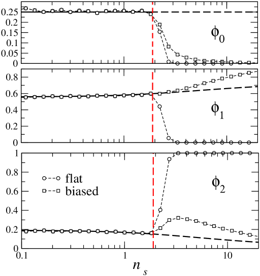
Figure 1: Top to bottom: the fraction of speculators using $0$, $1$ and both of their strategies versus $n_{s}$ at $n_{p}=1$. Markers denote results of on-line simulations of systems with $N_{s}P=10^{4}$ averaged over $200$ disorder samples per point. ‘Flat’ refers to initial conditions with $U_{i,1}(0)=U_{i,2}(0)$ for all speculators $i$. ‘Biased’ denotes instead initial states with $U_{is}(0)=O(\sqrt{N})>0$ and $U_{is^{\prime}}(0)=0$. Continuous lines are analytic results, and they have been continued as dashed lines in the non-ergodic region. The dotted lines joining the markers are a guide for the eye. The dashed vertical line marks the critical point $n_{s}\simeq 1.88$ above which the ergodic theory breaks down.

The point where simulations and theory depart can be computed assuming that $\chi\to\infty$ (implying the onset of anomalous response). This gives the critical point $n_{s}\simeq 1.88$, above which the ergodicity assumptions fail and the steady state depends on initial conditions. Thus this model displays the standard phase transition with ergodicity breaking characterizing the original $S=1$ GCMG. Similarly to what happens in the canonical MG, the critical point (which in general depends on $n_{p}$), decreases as $S$ increases, a reflection of the fact that agents .

5 Generalisation to models with $K$ assets

Multi-asset Minority Games have been introduced in [5] but we shall discuss here a slightly more general version of the same model. One considers a market with $K$ assets $\sigma\in\mathbb{Z}_{K}\equiv\{1,\ldots,K\}$ and $N$ agents. At each time step $\ell$, agents receive $K$ information patterns $\mu_{\sigma}(t)\in\{1,\ldots,P_{\sigma}\}$ chosen randomly and independently for each $\sigma$ with uniform probability and, based on these, they formulate their bids (one bid per asset at each time step). $P_{\sigma}$ is taken to scale linearly with $N$ and we will denote their ratios as $\alpha_{\sigma}=P_{\sigma}/N$. For each asset $\sigma$, every agent disposes of $S$ trading strategies $\{a_{is\sigma}^{\mu_{\sigma}}\}_{s=1}^{S}$ that prescribe a binary action $a^{\mu_{\sigma}}_{is\sigma}\in\{-1,1\}$, drawn randomly and uniformly, and independently for each asset, strategy and pattern. The performance of every strategy foe each asset is monitored by a score function $U_{is\sigma}(\ell)$ which is updated by the following rule

$$U_{is\sigma}(\ell+1)=U_{is\sigma}(\ell)-a_{is\sigma}^{\mu_{\sigma}(\ell)}A_{\sigma}(\ell)-\epsilon_{is\sigma}/\sqrt{N}$$ (78)

where $\epsilon_{is\sigma}$ are real constants representing positive or negative incentives for the agents to trade, and $A_{\sigma}(\ell)$ is the excess demand of asset $\sigma$ at time $\ell$,

$$A_{\sigma}(\ell)=\frac{1}{\sqrt{N}}\sum_{j=1}^{N}b_{j\sigma}(\ell)$$ (79)

where $b_{i\sigma}(\ell)$ denotes the bid formulated by agent $i$ in asset $\sigma$ at time $\ell$. Let $\{s_{i\sigma}(\ell)\}_{\sigma\in\mathbb{Z}_{K}}$ be the strategies he chooses for each asset and let $\mathcal{T}_{i}(\ell)\subseteq\mathbb{Z}_{K}$ denote the subset of assets in which agent $i$ trades at time $\ell$. We then write the bid explicitly in the following form:

$$b_{i\sigma}(\ell)=\sum_{s=1}^{S}{\mbox{\boldmath{1}{I}}}_{\sigma\in\mathcal{T}_{i}(\ell)}a_{is\sigma}^{\mu_{\sigma}(\ell)}\delta_{s,s_{i\sigma}(\ell)}n_{is\sigma}(\ell)$$ (80)

Here, the terms $a_{is\sigma}^{\mu_{\sigma}(\ell)}\delta_{s,s_{i\sigma}(\ell)}n_{is\sigma}(\ell)$ preserve the meaning they had in the single-asset model. The new term

$${\mbox{\boldmath{1}{I}}}_{\sigma\in\mathcal{T}}=\left\{\begin{array}[]{cl}1&\sigma\in\mathcal{T}\subseteq\mathbb{Z}_{K}\\ 0&{\rm otherwise}\end{array}\right.$$ (81)

defines the set of assets in which agent $i$ is active. We assume now that

$$\mathcal{T}_{i}(\ell)=h_{i}[\{U_{is\sigma}(\ell)\}]$$ (82)

$$s_{i\sigma}(\ell)=g_{i}[\{U_{is\sigma}(\ell)\}]$$ (83)

with $\{g_{i}\}$ and $\{h_{i}\}$ generic functions describing the strategy and asset selection rule. In the model described in [5], $S=1$ and $K=2$ with $\mathcal{T}_{i}(\ell)=\{\widetilde{\sigma}\in\mathbb{Z}_{2}{\rm~{}s.t.~{}}\widetilde{\sigma}={\rm arg~{}}\max_{\sigma}U_{is\sigma}(\ell)\delta_{s,s_{i\sigma}(\ell)}\}$.

The batch dynamics can be analysed in terms of $SK$ effective processes for a single representative agent:

$$U_{s\sigma}(t+1) = U_{s\sigma}(t)+\theta_{\sigma}(t)-\alpha_{\sigma}\epsilon_{s\sigma}$$ (84)

$$-\alpha_{\sigma}\sum_{t^{\prime}\leq t}[{\mbox{\boldmath{1}{I}}}+G_{\sigma}]^{-1}(t,t^{\prime})n_{s\sigma}(t^{\prime}){\mbox{\boldmath{1}{I}}}_{\sigma\in\mathcal{T}(t^{\prime})}\delta_{s_{\sigma}(t^{\prime}),s}+\eta_{s\sigma}(t)\,,$$

where $\{\eta_{s\sigma}(t)\}$ is again a coloured Gaussian noise, viz.

$$\left\langle\eta_{s\sigma}(t)\right\rangle_{\star}=0$$ (85)

$$\left\langle\eta_{s\sigma}(t)\eta_{s^{\prime}\sigma^{\prime}}(t^{\prime})\right\rangle_{\star}=\delta_{s,s^{\prime}}\delta_{\sigma,\sigma^{\prime}}\alpha_{\sigma}[({\mbox{\boldmath{1}{I}}}+G_{\sigma})^{-1}C_{\sigma}({\mbox{\boldmath{1}{I}}}+G^{\dagger}_{\sigma})^{-1}](t,t^{\prime})$$ (86)

and where

$$C_{\sigma}(t,t^{\prime})=\sum_{s=1}^{S}\int d{\mbox{\boldmath$\epsilon$}}\,w({\mbox{\boldmath$\epsilon$}})\int dgdh\,W[g,h]\,\left\langle n_{s\sigma}(t)n_{s\sigma}(t^{\prime})\delta_{s,s_{\sigma}(t)}\delta_{s,s_{\sigma}(t^{\prime})}{\mbox{\boldmath{1}{I}}}_{\sigma\in\mathcal{T}(t)}{\mbox{\boldmath{1}{I}}}_{\sigma\in\mathcal{T}(t^{\prime})}\right\rangle_{\star}$$ (87)

$$G_{\sigma}(t,t^{\prime})=\sum_{s=1}^{S}\int d{\mbox{\boldmath$\epsilon$}}\,w({\mbox{\boldmath$\epsilon$}})\int dgdh\,W[g,h]\,\frac{\delta\left\langle n_{s\sigma}(t)\delta_{s,s_{\sigma}(t)}{\mbox{\boldmath{1}{I}}}_{\sigma\in\mathcal{T}(t)}\right\rangle_{\star}}{\delta\theta_{s\sigma}(t^{\prime})}$$ (88)

are identified with the bid autocorrelation and response functions of asset $\sigma$:

$$C_{\sigma}(t,t^{\prime})=\frac{1}{N}\sum_{i=1}^{N}\left[\left\langle b_{i\sigma}(t)b_{i\sigma}(t^{\prime})\right\rangle\right]_{dis}$$ (89)

$$G_{\sigma}(t,t^{\prime})=\frac{1}{N}\sum_{i=1}^{N}\left[\frac{\partial\left\langle b_{i\sigma}(t)\right\rangle}{\partial\theta_{i\sigma}(t^{\prime})}\right]_{dis}$$ (90)

in the limit $N\to\infty$. In the above formulas, $W[g,h]$ generalizes (5) to include the function $h_{i}$:

$$W[g,h]=\frac{1}{N}\sum_{i\in\mathbb{Z}_{N}}\delta_{(F)}(g-g_{i})\delta_{(F)}(h-h_{i})$$ (91)

Proceeding as before, one arrives (with obvious notation) at the following stationary state process:

$$u_{s\sigma}=\overline{\theta}_{\sigma}+\overline{\eta}_{\sigma}-\alpha_{\sigma}\epsilon_{s\sigma}-m_{\sigma}\sum_{\mathcal{T}\subseteq\mathbb{Z}_{K}}\sum_{n\in\mathcal{I}}nf_{ns\sigma}(\mathcal{T})$$ (92)

with

$$m_{\sigma}=\frac{\alpha_{\sigma}}{1+\chi_{\sigma}},~{}~{}~{}~{}~{}\left\langle\overline{\eta}_{s\sigma}^{2}\right\rangle\equiv\varsigma_{\sigma}^{2}=\frac{\alpha_{\sigma}c_{\sigma}}{(1+\chi_{\sigma})^{2}}$$ (93)

$$f_{ns\sigma}(\mathcal{T})=\lim_{\tau\to\infty}\frac{1}{\tau}\sum_{t=0}^{\tau-1}\delta_{\mathcal{T},\mathcal{T}(t)}{\mbox{\boldmath{1}{I}}}_{\sigma\in\mathcal{T}}\delta_{n,n_{s\sigma}(t)}\delta_{s_{\sigma}(t),s}$$ (94)

and where the asset-dependent persistent autocorrelation and susceptibility are given by

$$c_{\sigma} = \sum_{s=1}^{S}\sum_{\mathcal{T},\mathcal{T}^{\prime}\subseteq\mathbb{Z}_{K}}\sum_{n,n^{\prime}\in\mathcal{I}}n\,n^{\prime}\int d{\mbox{\boldmath$\epsilon$}}\,w({\mbox{\boldmath$\epsilon$}})\int dgdh\,W[g,h]\,\left\langle f_{ns\sigma}(\mathcal{T})f_{n^{\prime}s\sigma}(\mathcal{T}^{\prime})\right\rangle_{\star}$$ (95)

$$\chi_{\sigma} = \frac{1}{\varsigma^{2}_{\sigma}}\sum_{s=1}^{S}\sum_{\mathcal{T}\subseteq\mathbb{Z}_{K}}\sum_{n\in\mathcal{I}}n\int d{\mbox{\boldmath$\epsilon$}}\,w({\mbox{\boldmath$\epsilon$}})\int dfdg\,W[f,g]\,\left\langle\overline{\eta}_{s\sigma}f_{ns\sigma}(\mathcal{T})\right\rangle_{\star}$$ (96)

Given a subset of assets $\mathcal{T}$, then $f_{ns\sigma}(\mathcal{T})$ is the frequency of the asset $\sigma\in\mathcal{T}$ being traded by using the strategy $s$ when an action $n$ has been taken on the market. The normalization now reads

$$\sum_{\mathcal{T}\in\mathbb{Z}_{K}}\frac{1}{|\mathcal{T}|}\sum_{\sigma\in\mathcal{T}}\sum_{n\in\mathcal{I}}\sum_{s\in\mathbb{Z}_{S}}f_{ns\sigma}(\mathcal{T})=1$$ (97)

Let us discuss the simplest case in which $F\equiv 1$ and $S=1$, corresponding to the canonical multi-asset MG (whose particular case $K=2$ is the subject of [5]). Agents have at their disposal a set of $K$ assets to trade, one each time (i.e. $|\mathcal{T}|=1$). We assume that $\epsilon_{s\sigma}=\epsilon_{\sigma}$ and that the asset selected at time $t$ is given by

$$\sigma(t)=h[\{U_{\sigma}(t)\}]={\rm arg\,max}_{\sigma}[\{u_{\sigma}(t)\}]$$ (98)

Following the same line of arguments one obtains the following expression for the distribution of frequencies for a subset of assets $\mathcal{T}$ being traded in the steady state:

$$\varrho_{\mathcal{T}}(u,\textbf{f})=\sum_{(\sigma_{1},\ldots,\sigma_{|\mathcal{T}|-1})\subset\mathcal{T}}m_{\sigma_{1}}\cdots m_{\sigma_{|\mathcal{T}|-1}}\delta\left(\sum_{\sigma\in\mathcal{T}}f_{\sigma}-1\right)\left[\prod_{\sigma\not\in\mathcal{T}}\delta_{f_{\sigma},0}\right]$$

$$\times P[\textbf{x}(u,\{f_{\sigma}\}_{\sigma\in\mathcal{T}})]\left\langle\prod_{\sigma\not\in\mathcal{T}}\Theta\left(u-y_{\sigma}\right)\right\rangle_{\textbf{y}}$$ (99)

where

$$x_{\sigma}\left(u,\{f_{\sigma}\}_{\sigma\in\mathcal{T}}\right)\equiv u+m_{\sigma}f_{\sigma}-\alpha_{\sigma}\epsilon_{\sigma}$$ (100)

As before the frequency distribution is given by the sum over all possible partitions of $\mathbb{Z}_{K}$ (empty set not included):

$$\left\langle(\cdots)\right\rangle_{\star}=\sum_{\mathcal{T}\subseteq\mathbb{Z}_{K}|\mathcal{T}\neq\emptyset}\int du\,d\textbf{f}\,\varrho_{\mathcal{T}}(u,\textbf{f})\,(\cdots)$$ (101)

Within this framework, the persistent correlation and susceptibility read

$$c_{\sigma} = \sum_{\mathcal{T}\subseteq\mathbb{Z}_{K}|\mathcal{T}\neq\emptyset}\int du\,d\textbf{f}\,\varrho_{\mathcal{T}}(u,\textbf{f})f^{2}_{\sigma}\,,$$ (102)

$$\chi_{\sigma} = \frac{1}{\varsigma^{2}_{\sigma}}\sum_{\mathcal{T}\subseteq\mathbb{Z}_{K}|\mathcal{T}\neq\emptyset}\int du\,d\textbf{f}\,\varrho_{\mathcal{T}}(u,\textbf{f})\,[x_{\sigma}(u,\{f_{\sigma}\}_{\sigma\in\mathcal{T}})f_{\sigma}]$$ (103)

whereas the fraction $\phi_{\mathcal{T}}$ of agents trading a certain subset $\mathcal{T}$ reads

$$\phi_{\mathcal{T}}=\int du\,d\textbf{f}\,\varrho_{\mathcal{T}}(u,\textbf{f})$$ (104)

It is easily checked that $\phi_{\mathcal{T}}$ satisfies $\sum_{\mathcal{T}\subseteq\mathbb{Z}_{K}|\mathcal{T}\neq\emptyset}\phi_{\mathcal{T}}=1$.

6 Summary and outlook

Minority Games with $S$ strategies and/or $K$ assets per agent are intriguing generalizations of the standard MG setup which display a qualitatively similar global physical picture (e.g. regarding the transition with ergodicity breaking) but substantially richer patterns of agent behaviour, directly related to the enlargement of the agents’ strategic endowments. The precise characterization of this aspect, even in the ergodic regime, poses challenging technical problems which have started to be analysed only recently. The central issue concerns the calculation of the statistics of the frequencies with which subsets of strategies are used. This problem was first tackled in [3], where an explicit solution is derived in the context of canonical batch MGs. In this work we have presented an alternative and mathematically simpler solution method (though the complexity of the calculations still increases rapidly with $S$). We have shown specifically how to recover the theory of the canonical case and solved explicitly the grand-canonical batch MG with $S$ strategies per agent. The method also generalizes to the recently introduced multi-asset models.

The method discussed here can be applied to a number of variants of the basic setup, some of which may be important from an economic viewpoint (for example in order to study the emergence of cross-asset correlations). Its main limitation is that, while the effective-agent dynamics, eqn. (10), holds true in both the ergodic and non-ergodic phases, our futher focus on time-translational properties limits the rigour of our conclusions to the ergodic regime. The richness of the MG dynamics is actually most striking when ergodicity is broken. Multi-strategy MGs are likely to produce a variety of possible steady states that may require novel observables to be completely characterised. Up to now, our understanding of non-ergodic regimes relies entirely on ad hoc heuristic arguments (see for instance [8, 11]) which provide a rough picture of the geometry of steady states and of the role of initial conditions for obtaining states of high or low volatility, but a more precise characterization remains elusive. In our opinion, at the present stage of our theoretical understanding of MGs, any advance in this direction would be most welcome.

References

References

[1]Challet D, Marsili M and Zhang YC 2005 Minority Games
(Oxford University Press, Oxford)
[2]Coolen ACC 2005 The mathematical theory of Minority
Games (Oxford University Press, Oxford)
[3]Shayeghi N and Coolen ACC 2006 J. Phys. A:
Math. Gen.39 13921
[4]Challet D and Marsili M 2003 Phys. Rev. E68
036132
[5]Bianconi G, De Martino A, Ferreira FF and Marsili M 2006
Preprint physics/0603152
[6]De Martino A and Marsili M 2006 J. Phys. A: Math.
Gen.39 R465
[7]Coolen ACC, Heimel JAF and Sherrington D 2001 Phys. Rev. E65 016126
[8]Heimel JAF and Coolen ACC 2001 Phys. Rev. E63 056121
[9]De Dominicis C 1978 Phys. Rev. B18 4913
[10]Challet D, De Martino A, Marsili M and Perez Castillo
I 2006 JSTAT P03004
[11]Marsili M and Challet D 2001 Phys. Rev. E64
056138