A stochastic representation for the Poisson-Vlasov equation

Abstract

A stochastic representation for the solutions of the Poisson-Vlasov equation is obtained. The representation involves both an exponential and a branching process. The stochastic representation, besides providing an alternative existence proof and an intuitive characterization of the solutions, may also be used to obtain an intrinsic definition of the fluctuations.

1 Introduction

The solutions of linear elliptic and parabolic equations, both with Cauchy and Dirichlet boundary conditions, have a probabilistic interpretation, which not only provides intuition on the nature of the problems described by these equations, but is also quite useful in the proof of general theorems. This is a very classical field which may be traced back to the work of Courant, Friedrichs and Lewy [1] in the 20’s. In spite of the pioneering work of McKean [2], the question of whether useful probabilistic representations could also be found for a large class of nonlinear equations remained an essentially open problem for many years.

It was only in the 90’s that, with the work of Dynkin[3] [4], such a theory started to take shape. For nonlinear diffusion processes, the branching exit Markov systems, that is, processes that involve diffusion and branching, seem to play the same role as Brownian motion in the linear equations. However the theory is still limited to some classes of nonlinearities and there is much room for further mathematical improvement.

Another field, where considerable recent advances were achieved, was the probabilistic representation of the Fourier transformed Navier-Stokes equation, first with the work of LeJan and Sznitman[5], later followed by extensive developments of the Oregon school[6] [7] [8]. In all cases the stochastic representation defines a process for which the mean values of some functionals coincide with the solution of the deterministic equation.

Stochastic representations, in addition to its intrinsic mathematical relevance, have several practical implications:

(i) They provide an intuitive characterization of the equation solutions;

(ii) They provide a calculation tool which may replace, for example, the need for very fine integration grids at high Reynolds numbers;

(iii) By associating a stochastic process to the solutions of the equation, they provide an intrinsic characterization of the nature of the fluctuations associated to the physical system. In some cases the stochastic process is essentially unique, in others there is a class of processes with means leading to the same solution. The physical significance of this feature is worth exploring.

A field where stochastic representations have not yet been developed (and where for the practical applications cited above they might be useful) is the field of kinetic equations for charged fluids. As a first step towards this goal, a stochastic representation is here constructed for the solutions of the Poisson-Vlasov equation.

The comments in the final section point towards future work, in particular on how a stochastic representation may be used for a characterization of fluctuations, alternative to existing methods. This is what we call the stochastic principle.

2 Stochastic representation and existence

Consider a Poisson-Vlasov equation in 3+1 space-time dimensions

$$\frac{\partial f}{\partial t}+\stackrel{{\scriptstyle\rightarrow}}{{v}}\cdot\nabla_{x}f-\frac{e}{m}\nabla_{x}\Phi\cdot\nabla_{v}f=0$$ (1)

with

$$\Delta_{x}\Phi_{f}=-4\pi\left\{e\int f\left(\stackrel{{\scriptstyle\rightarrow}}{{x}},\stackrel{{\scriptstyle\rightarrow}}{{v}},t\right)d^{3}v-e\rho_{B}\left(\stackrel{{\scriptstyle\rightarrow}}{{x}}\right)\right\}$$ (2)

$\rho_{B}\left(\stackrel{{\scriptstyle\rightarrow}}{{x}}\right)$ being a background charge density.

Passing to the Fourier transform

$$F\left(\xi,t\right)=\frac{1}{\left(2\pi\right)^{3}}\int d^{6}\eta f\left(\eta,t\right)e^{i\xi\cdot\eta}$$ (3)

with $\eta=\left(\stackrel{{\scriptstyle\rightarrow}}{{x}},\stackrel{{\scriptstyle\rightarrow}}{{v}}\right)$ and $\xi=\left(\stackrel{{\scriptstyle\rightarrow}}{{\xi_{1}}},\stackrel{{\scriptstyle\rightarrow}}{{\xi_{2}}}\right)\circeq\left(\xi_{1},\xi_{2}\right)$, one obtains

$$0 = \frac{\partial F\left(\xi,t\right)}{\partial t}-\stackrel{{\scriptstyle\rightarrow}}{{\xi_{1}}}\cdot\nabla_{\xi_{2}}F\left(\xi,t\right)$$

$$+\frac{4\pi e^{2}}{m}\int d^{3}\xi_{1}^{{}^{\prime}}F\left(\xi_{1}-\xi_{1}^{{}^{\prime}},\xi_{2},t\right)\frac{\stackrel{{\scriptstyle\rightarrow}}{{\xi_{2}}}\cdot\stackrel{{\scriptstyle\rightarrow}}{{\xi_{1}^{{}^{\prime}}}}}{\left|\xi_{1}^{{}^{\prime}}\right|^{2}}\left\{F\left(\xi_{1}^{{}^{\prime}},0,t\right)-\frac{\stackrel{{\scriptstyle\char 126\relax}}{{\rho}}_{B}\left(\xi_{1}^{{}^{\prime}}\right)}{\left(2\pi\right)^{3/2}}\right\}$$

$\stackrel{{\scriptstyle\char 126\relax}}{{\rho}}_{B}\left(\xi_{1}^{{}^{\prime}}\right)$ being the Fourier transform of $\rho_{B}\left(x\right)$. Changing variables to

$$\tau=\gamma\left(\left|\xi_{2}\right|\right)t$$ (5)

where $\gamma\left(\left|\xi_{2}\right|\right)$ is a positive continuous function satisfying

$$\begin{array}[]{lllll}\gamma\left(\left|\xi_{2}\right|\right)=1&&\textnormal{if}&&\left|\xi_{2}\right|<1\\ \gamma\left(\left|\xi_{2}\right|\right)\geq\left|\xi_{2}\right|&&\textnormal{if}&&\left|\xi_{2}\right|\geq 1\end{array}$$

leads to

$$\frac{\partial F\left(\xi,\tau\right)}{\partial\tau} = \frac{\stackrel{{\scriptstyle\rightarrow}}{{\xi_{1}}}}{\gamma\left(\left|\xi_{2}\right|\right)}\cdot\nabla_{\xi_{2}}F\left(\xi,\tau\right)-\frac{4\pi e^{2}}{m}\int d^{3}\xi_{1}^{{}^{\prime}}F\left(\xi_{1}-\xi_{1}^{{}^{\prime}},\xi_{2},\tau\right)$$ (6)

$$\times\frac{\stackrel{{\scriptstyle\rightarrow}}{{\xi_{2}}}\cdot\stackrel{{\scriptstyle\char 94\relax}}{{\xi_{1}^{{}^{\prime}}}}}{\gamma\left(\left|\xi_{2}\right|\right)\left|\xi_{1}^{{}^{\prime}}\right|}\left\{F\left(\xi_{1}^{{}^{\prime}},0,\tau\right)-\frac{\stackrel{{\scriptstyle\char 126\relax}}{{\rho}}_{B}\left(\xi_{1}^{{}^{\prime}}\right)}{\left(2\pi\right)^{3/2}}\right\}$$

with $\stackrel{{\scriptstyle\char 94\relax}}{{\xi_{1}}}=\frac{\stackrel{{\scriptstyle\rightarrow}}{{\xi_{1}}}}{\left|\xi_{1}\right|}$. Eq.(6) written in integral form, is

$$F\left(\xi,\tau\right) = e^{\tau\frac{\stackrel{{\scriptstyle\rightarrow}}{{\xi_{1}}}}{\gamma\left(\left|\xi_{2}\right|\right)}\cdot\nabla_{\xi_{2}}}F\left(\xi_{1},\xi_{2},0\right)-\frac{4\pi e^{2}}{m}\int_{0}^{\tau}dse^{\left(\tau-s\right)\frac{\stackrel{{\scriptstyle\rightarrow}}{{\xi_{1}}}}{\gamma\left(\left|\xi_{2}\right|\right)}\cdot\nabla_{\xi_{2}}}$$

$$\times\int d^{3}\xi_{1}^{{}^{\prime}}F\left(\xi_{1}-\xi_{1}^{{}^{\prime}},\xi_{2},s\right)\frac{\stackrel{{\scriptstyle\rightarrow}}{{\xi_{2}}}\cdot\stackrel{{\scriptstyle\char 94\relax}}{{\xi_{1}^{{}^{\prime}}}}}{\gamma\left(\left|\xi_{2}\right|\right)\left|\xi_{1}^{{}^{\prime}}\right|}\left\{F\left(\xi_{1}^{{}^{\prime}},0,s\right)-\frac{\stackrel{{\scriptstyle\char 126\relax}}{{\rho}}_{B}\left(\xi_{1}^{{}^{\prime}}\right)}{\left(2\pi\right)^{3/2}}\right\}$$

For convenience, a stochastic representation is going to be written for the following function

$$\chi\left(\xi_{1},\xi_{2},\tau\right)=e^{-\lambda\tau}\frac{F\left(\xi_{1},\xi_{2},\tau\right)}{h\left(\xi_{1}\right)}$$ (8)

with $\lambda$ a constant and $h\left(\xi_{1}\right)$ a positive function to be specified later on. The integral equation for $\chi\left(\xi_{1},\xi_{2},\tau\right)$ is

$$\chi\left(\xi_{1},\xi_{2},\tau\right) = e^{-\lambda\tau}\chi\left(\xi_{1},\xi_{2}+\tau\frac{\xi_{1}}{\gamma\left(\left|\xi_{2}\right|\right)},0\right)-\frac{8\pi e^{2}}{m\lambda}\frac{\left(\left|\xi_{1}\right|^{-1}h*h\right)\left(\xi_{1}\right)}{h\left(\xi_{1}\right)}\int_{0}^{\tau}ds\lambda e^{-\lambda s}$$ (9)

$$\times\int d^{3}\xi_{1}^{{}^{\prime}}p\left(\xi_{1},\xi_{1}^{{}^{\prime}}\right)\chi\left(\xi_{1}-\xi_{1}^{{}^{\prime}},\xi_{2}+s\frac{\xi_{1}}{\gamma\left(\left|\xi_{2}\right|\right)},\tau-s\right)$$

$$\times\frac{\stackrel{{\scriptstyle\rightarrow}}{{\xi_{2}}}\cdot\stackrel{{\scriptstyle\char 94\relax}}{{\xi_{1}^{{}^{\prime}}}}}{\gamma\left(\left|\xi_{2}\right|\right)}\left\{\frac{1}{2}e^{\lambda\left(\tau-s\right)}\chi\left(\xi_{1}^{{}^{\prime}},0,\tau-s\right)-\frac{1}{2}\frac{\stackrel{{\scriptstyle\char 126\relax}}{{\rho}}_{B}\left(\xi_{1}^{{}^{\prime}}\right)}{\left(2\pi\right)^{3/2}h\left(\xi_{1}^{{}^{\prime}}\right)}\right\}$$

with

$$\left(\left|\xi_{1}\right|^{-1}h*h\right)=\int d^{3}\xi_{1}^{{}^{\prime}}\left|\xi_{1}^{{}^{\prime}}\right|^{-1}h\left(\xi_{1}-\xi_{1}^{{}^{\prime}}\right)h\left(\xi_{1}^{{}^{\prime}}\right)$$ (10)

and

$$p\left(\xi_{1},\xi_{1}^{{}^{\prime}}\right)=\frac{\left|\xi_{1}^{{}^{\prime}}\right|^{-1}h\left(\xi_{1}-\xi_{1}^{{}^{\prime}}\right)h\left(\xi_{1}^{{}^{\prime}}\right)}{\left(\left|\xi_{1}\right|^{-1}h*h\right)}$$ (11)

Eq.(9) has a stochastic interpretation as an exponential process (with a time shift in the second variable) plus a branching process. $p\left(\xi_{1},\xi_{1}^{{}^{\prime}}\right)d^{3}\xi_{1}^{{}^{\prime}}$ is the probability that, given a $\xi_{1}$ mode, one obtains a $\left(\xi_{1}-\xi_{1}^{{}^{\prime}},\xi_{1}^{{}^{\prime}}\right)$ branching with $\xi_{1}^{{}^{\prime}}$ in the volume $\left(\xi_{1}^{{}^{\prime}},\xi_{1}^{{}^{\prime}}+d^{3}\xi_{1}^{{}^{\prime}}\right)$. $\chi\left(\xi_{1},\xi_{2},\tau\right)$ is computed from the expectation value of a multiplicative functional associated to the processes. Convergence of the multiplicative functional hinges on the fulfilling of the following conditions :

(A) $\left|\frac{F\left(\xi_{1},\xi_{2},0\right)}{h\left(\xi_{1}\right)}\right|\leq 1$

(B) $\left|\frac{\stackrel{{\scriptstyle\char 126\relax}}{{\rho}}_{B}\left(\xi_{1}\right)}{\left(2\pi\right)^{3/2}h\left(\xi_{1}\right)}\right|\leq 1$

(C) $\left(\left|\xi_{1}\right|^{-1}h*h\right)\leq h\left(\xi_{1}\right)$

Condition (C) is satisfied, for example, for

$$h\left(\xi_{1}\right)=\frac{c}{\left(1+\left|\xi_{1}\right|^{2}\right)^{2}}\hskip 28.45274pt\mathnormal{and}\hskip 28.45274ptc\leq\frac{1}{4\pi}$$ (12)

Indeed computing $\frac{1}{h\left(\xi_{1}\right)}\left(\left|\xi_{1}\right|^{-1}h*h\right)$ one obtains

$$\frac{1}{h\left(\xi_{1}\right)}\left(\left|\xi_{1}\right|^{-1}h*h\right)=4\pi c\int_{0}^{\infty}dr\frac{r}{\left(1+r^{2}\right)^{2}}\frac{\left(1+\left|\xi_{1}\right|^{2}\right)^{2}}{\left(1+\left(\left|\xi_{1}\right|-r\right)^{2}\right)\left(1+\left(\left|\xi_{1}\right|+r\right)^{2}\right)}$$ (13)

This integral is bounded by a constant for all $\left|\xi_{1}\right|$, therefore, choosing $c$ sufficiently small, condition (C) is satisfied.

Once $h\left(\xi_{1}\right)$ consistent with (C) is found, conditions (A) and (B) only put restrictions on the initial conditions and the background charge. Now one constructs the stochastic process $X\left(\xi_{1},\xi_{2},\tau\right)$.

Because $e^{-\lambda\tau}$ is the survival probability during time $\tau$ of an exponential process with parameter $\lambda$ and $\lambda e^{-\lambda s}ds$ the decay probability in the interval $\left(s,s+ds\right)$, $\chi\left(\xi_{1},\xi_{2},\tau\right)$ in Eq.(9) is obtained as the expectation value of a multiplicative functional for the following backward-in-time process:

Starting at $\left(\xi_{1},\xi_{2},\tau\right)$, a particle lives for an exponentially distributed time $s$ up to time $\tau-s$. At its death a coin $l_{s}$ (probabilities $\frac{1}{2},\frac{1}{2}$) is tossed. If $l_{s}=0$ two new particles are born at time $\tau-s$ with Fourier modes $\left(\xi_{1}-\xi_{1}^{{}^{\prime}},\xi_{2}+s\frac{\xi_{1}}{\gamma\left(\left|\xi_{2}\right|\right)}\right)$ and $\left(\xi_{1}^{{}^{\prime}},0\right)$ with probability density $p\left(\xi_{1},\xi_{1}^{{}^{\prime}}\right)$. If $l_{s}=1$ only the $\left(\xi_{1}-\xi_{1}^{{}^{\prime}},\xi_{2}+s\frac{\xi_{1}}{\gamma\left(\left|\xi_{2}\right|\right)}\right)$ particle is born and the process also samples the background charge at $\stackrel{{\scriptstyle\char 126\relax}}{{\rho}}_{B}\left(\xi_{1}^{{}^{\prime}}\right)$. Each one of the newborn particles continues its backward-in-time evolution, following the same death and birth laws. When one of the particles of this tree reaches time zero it samples the initial condition. The multiplicative functional of the process is the product of the following contributions:

- At each branching point where two particles are born, the coupling constant is

$$g_{2}\left(\xi_{1},\xi_{1}^{{}^{\prime}},s\right)=-e^{\lambda\left(\tau-s\right)}\frac{8\pi e^{2}}{m\lambda}\frac{\left(\left|\xi_{1}\right|^{-1}h*h\right)\left(\xi_{1}\right)}{h\left(\xi_{1}\right)}\frac{\stackrel{{\scriptstyle\rightarrow}}{{\xi_{2}}}\cdot\stackrel{{\scriptstyle\char 94\relax}}{{\xi_{1}^{{}^{\prime}}}}}{\gamma\left(\left|\xi_{2}\right|\right)}$$ (14)

- When only one particle is born and the process samples the background charge, the coupling is

$$g_{1}\left(\xi_{1},\xi_{1}^{{}^{\prime}}\right)=\frac{8\pi e^{2}}{m\lambda}\frac{\left(\left|\xi_{1}\right|^{-1}h*h\right)\left(\xi_{1}\right)}{h\left(\xi_{1}\right)}\frac{\stackrel{{\scriptstyle\char 126\relax}}{{\rho}}_{B}\left(\xi_{1}^{{}^{\prime}}\right)}{\left(2\pi\right)^{3/2}h\left(\xi_{1}^{{}^{\prime}}\right)}\frac{\stackrel{{\scriptstyle\rightarrow}}{{\xi_{2}}}\cdot\stackrel{{\scriptstyle\char 94\relax}}{{\xi_{1}^{{}^{\prime}}}}}{\gamma\left(\left|\xi_{2}\right|\right)}$$ (15)

- When one particle reaches time zero and samples the initial condition the coupling is

$$g_{0}\left(\xi_{1},\xi_{2}\right)=\frac{F\left(\xi_{1},\xi_{2},0\right)}{h\left(\xi_{1}\right)}$$ (16)

The multiplicative functional is the product of all these couplings for each realization of the process $X\left(\xi_{1},\xi_{2},\tau\right)$, this process being obtained as the limit of the following iterative process

$$X^{\left(k+1\right)}\left(\xi_{1},\xi_{2},\tau\right) = \chi\left(\xi_{1},\xi_{2}+\tau\frac{\xi_{1}}{\gamma\left(\left|\xi_{2}\right|\right)},0\right)\mathbf{1}_{\left[s>\tau\right]}+g_{2}\left(\xi_{1},\xi_{1}^{{}^{\prime}},s\right)$$

$$\times X^{\left(k\right)}\left(\xi_{1}-\xi_{1}^{{}^{\prime}},\xi_{2}+s\frac{\xi_{1}}{\gamma\left(\left|\xi_{2}\right|\right)},\tau-s\right)X^{\left(k\right)}\left(\xi_{1}^{{}^{\prime}},0,\tau-s\right)\mathbf{1}_{\left[s<\tau\right]}\mathbf{1}_{\left[l_{s}=0\right]}$$

$$+g_{1}\left(\xi_{1},\xi_{1}^{{}^{\prime}}\right)X^{\left(k\right)}\left(\xi_{1}^{{}^{\prime}},0,\tau-s\right)\mathbf{1}_{\left[s<\tau\right]}\mathbf{1}_{\left[l_{s}=1\right]}$$

Then, $\chi\left(\xi_{1},\xi_{2},\tau\right)$ is the expectation value of the functional.

$$\chi\left(\xi_{1},\xi_{2},\tau\right)=\mathbb{E}\left\{\Pi\left(g_{0}g_{0}^{{}^{\prime}}\cdots\right)\left(g_{1}g_{1}^{{}^{\prime}}\cdots\right)\left(g_{2}g_{2}^{{}^{\prime}}\cdots\right)\right\}$$ (17)

For example, for the realization in Fig.1 the contribution to the multiplicative functional is

$$g_{2}\left(\xi_{1},\xi_{1}^{{}^{\prime}},\tau-s_{1}\right)g_{2}\left(\xi_{1}^{{}^{\prime}},\xi_{1}^{{}^{\prime\prime\prime}},\tau-s_{3}\right)g_{1}\left(\xi_{1}-\xi_{1}^{{}^{\prime}},\xi_{1}^{{}^{{}^{\prime\prime}}}\right)$$

$$\times g_{0}\left(\xi_{1}-\xi_{1}^{{}^{\prime}}-\xi_{1}^{{}^{\prime\prime}},k_{2}\right)g_{0}\left(\xi_{1}^{{}^{\prime}}-\xi_{1}^{{}^{\prime\prime\prime}},k_{3}\right)g_{0}\left(\xi_{1}^{{}^{{}^{\prime\prime\prime}}},0\right)$$

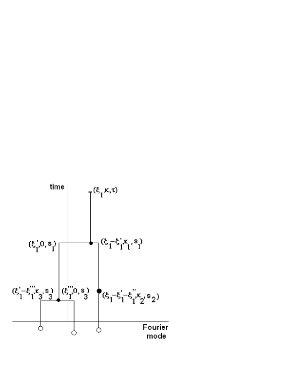
Figure 1: A sample path of the stochastic process

and

$$\begin{array}[]{lll}k&=&\xi_{2}\\ k_{1}&=&k+s_{1}\frac{\xi_{1}}{\gamma\left(\left|\xi_{2}\right|\right)}\\ k_{2}&=&k_{1}+\left(s_{2}-s_{1}\right)\frac{\left(\xi_{1}-\xi_{1}^{{}^{\prime}}\right)}{\gamma\left(\left|k_{1}\right|\right)}\\ k_{3}&=&\left(s_{3}-s_{1}\right)\xi_{1}^{{}^{\prime}}\end{array}$$

With the conditions (A) and (B), choosing

$$\lambda=\frac{8\pi e^{2}}{m}$$

and

$$c\leq e^{-\lambda\tau}\frac{1}{4\pi}$$

the absolute value of all coupling constants is bounded by one. The branching process, being identical to a Galton-Watson process, terminates with probability one and the number of inputs to the functional is finite (with probability one). With the bounds on the coupling constants, the multiplicative functional is bounded by one in absolute value almost surely.

Once a stochastic representation is obtained for $\chi\left(\xi_{1},\xi_{2},\tau\right)$, one also has, by (8), a stochastic representation for the solution of the Fourier-transformed Poisson-Vlasov equation. The results are summarized in the following :

Theorem 2.1 - There is a stochastic representation for the Fourier-transformed solution of the Poisson-Vlasov equation $F\left(\xi_{1},\xi_{2},t\right)$ for any arbitrary finite value of the arguments, provided the initial conditions at time zero and the background charge satisfy the boundedness conditions (A) and (B).

As a corollary one also infers an existence result for (arbitrarily large) finite time. Notice that existence by the stochastic representation method requires only boundedness conditions on the initial conditions and background charge and not any strict smoothness properties.

3 Fluctuations and the stochastic principle. A comment

In the past, the fluctuation spectrum of charged fluids was studied either by the BBGKY hierarchy derived from the Liouville or Klimontovich equations, with some sort of closure approximation, or by direct approximations to the N-body partition function or by models of dressed test particles, etc. (see reviews in [9] [10]). Alternatively, by linearizing the Vlasov equation about a stable solution and diagonalizing the Hamiltonian, a canonical partition function may be used to compute correlation functions [11].

However, one should remember that, as a model for charged fluids, the Vlasov equation is just a mean-field collisionless theory. Therefore, it is unlikely that, by itself, it will contain full information on the fluctuation spectrum. Kinetic and fluid equations are obtained from the full particle dynamics in the 6N-dimensional phase-space by a chain of reductions. Along the way, information on the actual nature of fluctuations and turbulence may have been lost. An accurate model of turbulence may exist at some intermediate (mesoscopic) level, but not necessarily in the final mean-field equation.

When a stochastic representation is constructed, one obtains a process for which the mean value is the solution of the mean-field equation. The process itself contains more information. This does not mean, of course, that the process is an accurate mesoscopic model of Nature, because we might be climbing up a path different from the one that led us down from the particle dynamics.

Nevertheless, insofar as the stochastic representation is qualitatively unique and related to some reasonable iterative process, it provides a surrogate mesoscopic model from which fluctuations are easily computed. This is what we refer to as the stochastic principle. At the minimum, one might say that the stochastic principle provides another closure procedure.

References

[1] R. Courant, K. Friedrichs and H. Lewy; Mat. Ann. 100
(1928) 32-74.
[2] H. P. McKean; Comm. Pure Appl. Math. 28 (1975) 323-331, 29
(1976) 553-554.
[3] E. B. Dynkin; Prob. Theory Rel. Fields 89 (1991) 89-115.
[4] E. B. Dynkin; Diffusions, Superdiffusions and
Partial Differential Equations,AMS Colloquium Pubs., Providence 2002.
[5] Y. LeJan and A. S. Sznitman ; Prob. Theory and Relat. Fields
109 (1997) 343-366.
[6] E. C. Waymire; Prob. Surveys 2 (2005) 1-32.
[7] R. N. Bhattacharya et al. ; Trans. Amer. Math. Soc. 355
(2003) 5003-5040
[8] M. Ossiander ; Prob. Theory and Relat. Fields 133
(2005) 267-298.
[9] C. R. Oberman and E. A. Williams; in Handbook of
Plasma Physics (M. N. Rosenbluth, R. Z. Sagdeev, Eds.), pp. 279-333,
North-Holland, Amsterdam 1985.
[10] J. A. Krommes; Phys. Reports 360 (2002) 1-352.
[11] P. J. Morrison; Phys. of Plasmas 12 (2005) 058102.