Magnetophoresis of nonmagnetic particles in ferrofluids

Abstract

Ferrofluids containing nonmagnetic particles are called inverse ferrofluids. Based on the Ewald-Kornfeld formulation and the Maxwell-Garnett theory, we theoretically investigate the magnetophoretic force exerting on the nonmagnetic particles in inverse ferrofluids due to the presence of a nonuniform magnetic field, by taking into account the structural transition and long-range interaction. We numerically demonstrate that the force can be adjusted by choosing appropriate lattices, volume fractions, geometric shapes, and conductivities of the nonmagnetic particles, as well as frequencies of external magnetic fields.

I Introduction

Magnetizable particles experience a force in a nonuniform magnetic field, which comes from the interaction between the induced magnetic moment inside the particles and the external magnetic field. This phenomenon is called magnetophoresis,^1,2 and has been exploited in a variety of industrial and commercial process for separation and beneficiation of solids suspended in liquids.³ Magnetophoresis may also open up a way to characterize and separate cells for biochemical analysis based on intrinsic and extrinsic magnetic properties of biological macromolecules.⁴

Ferrofluids, also known as magnetic fluids, are a colloidal suspension of single-domain ferromagnetic nanoparticles (e.g., made of Fe₃O₄), with typical dimension around 10 nm, dispersed in a carrier liquid like water or kerosene.^3,5-7 Ferrofluids containing nonmagnetic particles (or magnetic holes) are called inverse ferrofluids. So far, inverse ferrofluids have drawn much attention for their potential industrial and biomedical applications.^8-11 The size of the nonmagnetic particles (such as polystyrene particles) is about 1$\sim$100 $\mu$m. Since the nonmagnetic particles are much larger than the ferromagnetic nanoparticles in host ferrofluids, the host can theoretically be treated as a one-component continuum in which the much larger nonmagnetic particles are embedded.^12,13 It is known that the ground state of electrorheological fluids and magnetorheological fluids is body-centered tetragonal (bct) lattices.^14,15 Due to mathematical analogy, the ground state of inverse ferrofluids might also be body-centered tetragonal (bct) lattices. Similar to electrorheological fluids,¹⁶ under appropriate conditions, such as by adjusting the application of external magnetic fields, structural transition may also appear in inverse ferrofluids, e.g., from the bct to the body-centered cubic (bcc), and then to the face-centered cubic (fcc) lattices.

When an external magnetic field is applied, the nonmagnetic particles in inverse ferrofluids can be seen to possess an effective magnetic moment, which, however, is anti-parallel to the magnetization of the host ferrofluid. In this sense, the nonmagnetic particles also experience an equivalent magnetophoretic force in the presence of a nonuniform magnetic field naturally. In this work, we shall apply a nonuniform magnetic field to investigate the magnetophoresis of the nonmagnetic particles in inverse ferrofluids with different structures of specific lattices.

One of us¹⁷ has investigated the dielectrophoretic force acting on a microparticle in electrorheological solids under the application of a nonuniform external electric field by using a self-consistent method¹⁸ and the spectral representation approach. In our present work, we shall use the Ewald-Kornfeld formulation and the Maxwell-Garnett theory for uniaxially anisotropic suspensions to calculate the effective permeability of the inverse ferrofluid, taking into account the long range interaction arising from specific lattices. Based on this, the magnetophoretic force acting on the nonmagnetic particles can be calculated accordingly. We shall focus on the role of types of lattices, volume fractions, geometric shapes, and conductivities of the nonmagnetic particles, as well as frequencies of external fields.

This paper is organized as follows. In Section II, we first briefly review the theory of magnetophoresis (Section II.1). By using the Ewald-Kornfeld formulation and the Maxwell-Garnett theory for uniaxially anisotropic suspensions, we calculate the effective permeability of the inverse ferrofluids (Section II.2). Then we investigate magnetophoresis with eddy current induction (Section II.3). In Section III, we give the numerical results under different conditions. This paper ends with a discussion and conclusions in Section IV.

II Formalism

II.1 Theory of magnetophoresis

To establish our theory, we first briefly review the theory of magnetophoresis (for details of magnetophoresis, we refer the reader to ref 1). Let us start by considering a homogeneous sphere with radius $R$ and magnetization $\mathbf{M}_{1}$ that is suspended in a magnetically linear fluid of permeability $\mu_{2}$ and subjected to a uniform magnetic field $\mathbf{H}_{0}$. The relation between magnetic flux density $\mathbf{B}$, magnetization $\mathbf{M}$, and magnetic intensity $\mathbf{H}$ is given by

$$\mathbf{B}=\mu_{0}(\mathbf{H}+\mathbf{M}),$$ (1)

where $\mu_{0}$ is the permeability of free space. Eq 1 is completely general, the magnetization $\mathbf{M}$ includes permanent magnetization plus any linear or nonlinear function of $\mathbf{H}$. $\mathbf{M}_{1}$ is assumed to be parallel to $\mathbf{H}_{0},$ $\mathbf{M}_{1}\|\mathbf{H}_{0}$. We also assume that no electric current flows anywhere. Thus, there is

$$\nabla\times\mathbf{H}=0$$ (2)

everywhere. Then, this magnetostatics problem may be solved using a scalar potential $\psi$, defined by $\mathbf{H}=-\nabla\psi$. The general solutions for $\psi_{1}$ and $\psi_{2}$ outside and inside the sphere are given by respectively,

$$\psi_{1}(r,\theta) = -H_{0}r\cos\theta+\frac{a\cos\theta}{r^{2}},\,\,\,r>R,$$ (3)

$$\psi_{2}(r,\theta) = -br\cos\theta,\,\,\,r<R.$$ (4)

The coefficients $a$ and $b$ can be determined by considering the appropriate boundary conditions,

$$a = \frac{\mu_{0}-\mu_{2}}{\mu_{0}+2\mu_{2}}R^{3}H_{0}+\frac{\mu_{0}}{\mu_{0}+2\mu_{2}}R^{3}M_{1},$$ (5)

$$b = \frac{3\mu_{2}}{\mu_{0}+2\mu_{2}}H_{0}-\frac{\mu_{0}}{\mu_{0}+2\mu_{2}}M_{1}.$$ (6)

It is worth noting that $b$ denotes the magnitude of the uniform magnetic field $H_{1}$ inside the sphere. We can determine the effective magnetic dipole moment $\mathbf{m}_{\mathrm{eff}}$ by comparing the dipole term in eq 3 with

$$\psi_{\mathrm{dipole}}=\frac{m_{\mathrm{eff}}\cos\theta}{4\pi r^{2}}.$$ (7)

Then, the effective magnetic moment is given by

$$\mathbf{m}_{\mathrm{eff}}=4\pi R^{3}\left[\frac{\mu_{0}-\mu_{2}}{\mu_{0}+2\mu_{2}}\mathbf{H}_{0}+\frac{\mu_{0}}{\mu_{0}+2\mu_{2}}\mathbf{M}_{1}\right].$$ (8)

For a magnetically linear particle of radius $R$ and permeability $\mu_{1}$ suspended in a host medium with permeability $\mu_{2}$, we have

$$\mathbf{M}_{1}=\chi_{1}\mathbf{H}_{1},$$ (9)

where $\chi_{1}=\mu_{1}/\mu_{0}-1$ is the susceptibility of the particle. In this case, the effective magnetic dipole moment vector $\mathbf{m}_{\mathrm{eff}}$ takes a form very similar to that for the effective dipole moment of dielectric spheres,

$$\mathbf{m}_{\mathrm{eff}}=4\pi R^{3}K(\mu_{1},\mu_{2})\mathbf{H}_{0},$$ (10)

where the Clausius-Mossotti factor $K(\mu_{1},\mu_{2})$ is given by,

$$K(\mu_{1},\mu_{2})=\frac{\mu_{1}-\mu_{2}}{\mu_{1}+2\mu_{2}}.$$ (11)

The magnetophoretic force exerted by a nonuniform magnetic field on a magnetic dipole can then be written as

$$F_{\mathrm{dipole}}=\mu_{2}\mathbf{m}_{\mathrm{eff}}\cdot{\bf\nabla}H_{0}.$$ (12)

Combining this expression with that for the effective magnetic dipole moment eq 10, the magnetophoretic force exerted on a magnetizable spherical particle in a nonuniform magnetic field is written as¹

$$F_{\mathrm{MAP}}=2\pi\mu_{2}R^{3}K(\mu_{1},\mu_{2})\nabla H_{0}^{2}.$$ (13)

Eq 13 is similar to the expression of the dielectrophoretic force on dielectric particles.^1,19 It is apparent to see that the magnetophoretic force are proportional to the particle volume and the permeability of the suspension medium. And the force is directed along the gradient of the external magnetic field. There are two kinds of magnetophoresis depending upon the relative magnitudes of $\mu_{1}$ and $\mu_{2}$. If $K>0$ (namely, $\mu_{1}>\mu_{2}$), particles are attracted to magnetic field intensity maxima and repelled from minima. This phenomenon is called positive magnetophoresis. On the contrary, if $K<0$ (i.e., $\mu_{1}<\mu_{2}$), inverse behavior appears, which is called negative magnetophoresis. Generally, there may be two magnetophoresis systems. One is that ferromagnetic particles are suspended in a medium that can be either nonmagnetic or less (linear) magnetizable, and the other one is that nonmagnetic particles are in a magnetizable liquid like ferrofluids. As for the second case of our interest in this work, in case of a moderate magnetic field (satisfying the assumption of a magnetically linear host), we can use eq 13 by setting $\mu_{1}=\mu_{0}$ to calculate the magnetophoretic force on the nonmagnetic particles submerged in a host ferrofluid.

II.2 Effective permeability

We resort to the Ewald-Kornfeld formulation to calculate the effective permeability by including the structural transition and corresponding long-range interaction explicitly. A bct lattice can be regarded as a tetragonal lattice, plus a basis of two particles each of which is fixed with an induced point magnetic dipole at its center. One of the two particles is located at a corner and the other one at the body center of the tetragonal unit cell. The tetragonal lattice has a lattice constant $c_{1}$= $\xi q$ along the $z$ axis and lattice constants $a_{1}=b_{1}=\xi q^{-\frac{1}{2}}$ along $x$ and $y$ axes, respectively. In this paper, we identify a different structure transformation from bct to bcc, and to fcc lattices by changing the uniaxial lattice constant $c_{1}$ under the hard-sphere constraint. The volume of the tetragonal unit cell $V_{c}$ remains unchanged (i. e., $V_{c}=\xi^{3}$) as $q$ varies. In this way, the degree of anisotropy of the tetragonal lattices is measured by how $q$ is deviated from unity and the uniaxial anisotropic axis is along the $z$ axis. In particular, $q=0.87358$, $1,$ and $2^{\frac{1}{3}}$ represent the bct, bcc, and fcc lattices, respectively.

When an external magnetic field $\mathbf{H}_{0}$ is directed along the $x$ axis, the induced magnetic moment $\mathbf{m}_{\rm eff}$ is perpendicular to the uniaxial anisotropic axis ($z$ axis). At the lattice point $\mathbf{R}={\bf 0}$, the local field $\mathbf{H}_{L}$ can be determined by using the Ewald-Kornfeld formulation,^20-22

$$\mathbf{H}_{L} = \mathbf{m}_{\rm eff}\sum_{j=1}^{2}\sum_{\mathbf{R}\neq 0}[-\gamma_{1}(R_{j})+x_{j}^{2}q^{2}\gamma_{2}(R_{j})]$$ (14)

$$-\frac{4\pi\mathbf{m}_{\rm eff}}{v_{c}}\sum_{\mathbf{G}\neq 0}\Pi(\mathbf{G})\frac{G_{x}^{2}}{G^{2}}\exp\left(\frac{-G^{2}}{4\eta^{2}}\right)+\frac{4\mathbf{m}_{\rm eff}\eta^{3}}{3\sqrt{\pi}}.$$

where $\gamma_{1}$ and $\gamma_{2}$ are two coefficients, given by

$$\gamma_{1}(r) = \frac{erfc(\eta r)}{r^{3}}+\frac{2\eta}{\sqrt{\pi}r^{2}}\exp(-\eta^{2}r^{2}),$$

$$\gamma_{2}(r) = \frac{3erfc(\eta r)}{r^{5}}+(\frac{4\eta^{3}}{\sqrt{\pi}r^{2}}+\frac{6\eta}{\sqrt{\pi}r^{4}})\exp-(\eta^{2}r^{2}),$$

where erfc$(\eta r)$ is the complementary error function, and $\eta$ is an adjustable parameter making the summations in real and reciprocal lattices converge rapidly. In eq 14, $\mathbf{R}$ and $\mathbf{G}$ denote the lattice vector and reciprocal lattice vector, respectively,

where $l,m,n,u,v,$ and $w$ are integers. In addition, $x_{j}$ and $R_{j}$ in eq 14 are given by

$$x_{j} = l-\frac{j-1}{2},$$

$$R_{j} = |\mathbf{R}-\frac{j-1}{2}(a_{1}\hat{\mathbf{x}}+a_{1}\hat{\mathbf{y}}+c_{1}\hat{\mathbf{z}})|,$$

and $\Pi(\mathbf{G})=1+\exp[i(u+v+w)/\pi]$ is the structure factor. The local magnetic field can be obtained by summing over all integer indices, $(u,v,w)\neq(0,0,0)$ for the summation in the reciprocal lattice, and $(j,l,m,n)\neq(1,0,0,0)$ for the summation in the real lattice. In our calculation, because of the exponential factors, we may impose an upper limit to the indices, i.e., all indices ranging from $-L$ to $L$, where $L$ is a positive integer. We consider an infinite lattice. So, for finite lattices, one must be careful about the effects of different boundary conditions.

Now, let us define a local field factor $\alpha$ as

$$\alpha=\frac{3}{4\pi}\frac{\mathbf{H}_{L}}{\sum_{V_{c}}\mathbf{m}_{\rm eff}/V_{c}}=\frac{3V_{c}}{8\pi}\frac{\mathbf{H}_{L}}{\mathbf{m}_{\rm eff}},$$ (15)

where $\sum_{V_{c}}\mathbf{m}_{\rm eff}=2{\bf m}_{\rm eff}$ means the sum of the two vector magnetic moments in the unit cell. It is worth remaking that $\alpha$ is a function of single variable $q$, and that it stands for $\alpha_{T}$ (local field factor in transverse field cases) and $\alpha_{L}$ (local field factor in longitudinal field cases) which satisfy a famous sum rule in condensed matter physics for $\alpha_{T}$ and $\alpha_{L}$, $2\alpha_{T}+\alpha_{L}=3$.^18,19 Here the longitudinal (transverse) field case corresponds to the fact that the external magnetic field is parallel (perpendicular) to the uniaxial anisotropic $z$ axis. Next, for calculating the effective permeability, we use the Maxwell-Garnett theory for uniaxially anisotropic suspensions,^23,24

$$\frac{\mu_{e}-\mu_{2}}{\alpha_{L,T}\mu_{e}+(3-\alpha_{L,T})\mu_{2}}=f\frac{\mu_{1}-\mu_{2}}{\mu_{1}+2\mu_{2}},$$ (16)

where $\mu_{e}$ stands for the effective permeability of the inverse ferrofluid, $\mu_{1}$ the permeability of the nonmagnetic particles, namely $\mu_{1}=\mu_{0},$ $\mu_{2}$ the permeability of the host ferrofluid, and $f$ the volume fraction of the nonmagnetic particles in the inverse ferrofluids.

It should be noted that eq 16 holds for the case of nonmagnetic particles with a spherical shape only. For nonspherical cases (e.g., prolate or oblate spheroids), we may use demagnetizing factor $g$ to describe the shape of different kinds of spheroids. For a prolate spheroid with three principal axes, $a$, $b$, and $c,$ there is $a=b<c,$ and the demagnetizing factor ${g}_{L}$ along the major axis $c$ is^25,26

$${g}_{L}=\frac{1}{k^{2}-1}\left[\frac{k}{\sqrt{k^{2}-1}}\ln(k+\sqrt{k^{2}-1})-1\right],$$ (17)

where $k=c/a>1$ and ${g}_{L}<1/3$. For an oblate spheroid with $a<b=c$, the demagnetizing factor ${g}_{L}$ along the major axis $a$ is^25,26

$${g}_{L}=1-\left[\frac{k^{2}}{(k^{2}-1)^{\frac{3}{2}}}\arcsin\frac{\sqrt{k^{2}-1}}{k}-\frac{1}{k^{2}-1}\right],$$ (18)

where $k=c/a>1$ and ${g}_{L}>1/3.$ For both cases, there is a geometrical sum rule for ${g}_{L}$ and ${g}_{T}$, $2{g}_{T}+{g}_{L}=1$, where ${g}_{T}$ denotes the demagnetizing factor along the minor axis. Note that the spherical shape of nonmagnetic particles corresponds to ${g}_{L}={g}_{T}=1/3.$ So far, to include the nonspherical shape effects, erq 16 for calculating the effective permeability of inverse ferrofluids containing spherical nonmagnetic particles might be modified as

$$\frac{\mu_{e}-\mu_{2}}{\mu_{2}+\frac{\alpha_{L,T}}{3}(\mu_{e}-\mu_{2})}=f\frac{\mu_{1}-\mu_{2}}{\mu_{2}+g_{L,T}(\mu_{1}-\mu_{2})}.$$ (19)

Apparently, the substitution of ${g}_{L}={g}_{T}=1/3$ into eq 19 reduces to eq 16.

II.3 Magnetophoresis with eddy current induction

When an ac (alternating current) magnetic field is applied to an electrically conductive magnetizable particle, eddy currents are induced, which tend to oppose penetration of the field into the particle. At sufficiently high frequencies, these eddy currents strongly influence the effective magnetic moment. Within the particle, $\nabla\times\mathbf{H}\neq 0.$ Similar derivation of this section can be found in ref 1 for a magnetic particle in a linear medium. Nevertheless, here we discuss a different system, thus yielding the following formulae with some difference.

Let us consider a nonmagnetic conductive particle with an effective magnetic dipole of magnitude $m_{\rm eff}$ [note that in this case there is ${\bf m}_{\rm eff}\|(-{\bf H}_{0})$ as mentioned in Section I], which is embedded in the system containing both a magnetically linear host ferrofluid and many other nonmagnetic conductive particles. In this case, the nonmagnetic particles are also assumed to situate in specific lattices and exist in the shape of spheres. The effective permeability of the whole system $\mu_{e}$ can be calculated according to eq 16. The magnetic vector potential ${\bf\Psi}$ at position $\mathbf{r}$ may be written as

$${\bf\Psi}=\frac{\mu_{e}\mathbf{m}_{\mathrm{eff}}\times\mathbf{r}}{4\pi r^{3}},$$ (20)

where ${\bf\nabla}\times{\bf\Psi}=\mathbf{B}$, $\mathbf{B}$ is the magnetic flux density. If we align the moment anti-parallel with $z$ axis, that is $\mathbf{m}_{\mathrm{eff}}=-m_{\mathrm{eff}}\hat{\mathbf{z}}.$ Then eq 20 can be rewritten as

$${\bf\Psi}=-\frac{\mu_{e}m_{\mathrm{eff}}\sin\theta}{4\pi r^{2}}\hat{{\bf\phi}},$$ (21)

where $\hat{{\bf\phi}}$ is the azimuthal unit vector in spherical coordinates. We consider a conductive nonmagnetic spherical particle of permeability $\mu_{1}(=\mu_{0})$ and conductivity $\sigma_{1}$, which is subjected to a uniform, linearly polarized magnetic field $\mathbf{H}(t)=H_{0}\cos\omega t\hat{\mathbf{z}}.$ The effective moment of the sphere can be written as

$$\mathbf{m}_{\mathrm{eff}}=-4\pi R^{3}L(\omega)H_{0}\hat{\mathbf{z}},$$ (22)

where $L(\omega)=R^{3}D/2$ is a frequency-dependent magnetization coefficient, and $D$ depends on $\mu_{e}$, $\mu_{1}$, $\sigma_{1}$, and $\omega$,

$$D=\frac{(2\mu_{1}+\mu_{e})\nu I_{-1/2}-[\mu_{e}(1+\nu^{2})+2\mu_{1}]I_{+1/2}}{(\mu_{1}-\mu_{e})\nu I_{-1/2}+[\mu_{e}(1+\nu^{2})-\mu_{1}]I_{+1/2}},$$ (23)

with $I_{\pm 1/2}=I_{\pm(\nu)}$ and $\nu=\sqrt{j\mu_{1}\sigma_{1}\omega R}$. The quantities $I_{\pm 1/2}$ are half-integer order, modified Bessel functions of the first kind. For a nonuniform ac magnetic field, according to the effective dipole method (see Sections II.1 and II.2), the time-average magnetophoretic force acting on a nonmagnetic conductive particle is

$$\langle F_{\mathrm{MAP}}(t)\rangle=\frac{\mu_{e}}{2}{\rm Re}[\mathbf{m}_{\mathrm{eff}}\cdot{\bf\nabla}H].$$ (24)

Next, we can obtain the expression for the magnetophoretic force in terms of the real part of $L$,

$$\langle F_{\mathrm{MAP}}(t)\rangle=-2\pi\mu_{e}R^{3}{\rm Re}[L]\nabla H_{0}^{2}.$$ (25)

A simplified expression for ${\rm Re}[L]$ may be obtained by invoking certain Bessel function identities,

$${\rm Re}[L]=\frac{3\mu_{R}}{2}\frac{(\mu_{R}-1)B^{2}+R_{m}^{2}(\sinh 2R_{m}-\sin 2R_{m})A}{(\mu_{R}-1)^{2}B^{2}+R_{m}^{2}A^{2}}-\frac{1}{2},$$ (26)

where $\mu_{R}=\mu_{1}/\mu_{e}$ is the relative permeability, $R_{m}=R\sqrt{\omega\mu_{1}\sigma_{1}/2}$ a dimensionless modulus called magnetic Reynolds number, and $A$ and $B$ are respectively given by

$$A = 2R_{m}(\cosh 2R_{m}-\cos 2R_{m})+(\mu_{R}-1)(\sinh 2R_{m}-\sin 2R_{m}),$$

$$B = \cosh 2R_{m}-\cos 2R_{m}-R_{m}(\sinh 2R_{m}+\sin 2R_{m}).$$

III Results

If the shape of the nonmagnetic particle is spherical, the magnetophoretic force on the nonmagnetic particle $F_{\mathrm{MAP}}$ can be calculated by

$$F_{\mathrm{MAP}} = 2\pi\mu_{e}R^{3}K(\mu_{1},\mu_{e})\nabla H_{0}^{2},$$ (27)

$$K(\mu_{1},\mu_{e}) = \frac{\mu_{1}-\mu_{e}}{\mu_{1}+2\mu_{e}}.$$ (28)

For obtaining eq 27, in order to include the lattice effect, $\mu_{2}$ in eq 13 has been replaced by $\mu_{e}$ that can be calculated according to eq 16. During the numerical calculation, for convenience, $F$ stands for $-F_{\rm{MAP}}/(2\pi R^{3}\nabla H_{0}^{2}).$ In our calculation, we choose the parameters $\mu_{1}=\mu_{0}$ and $\mu_{2}=2.9\mu_{0}.$ In this case, the parameter $K(\mu_{1},\mu_{e})<0$ corresponds to the phenomenon of negative magnetophoresis.

Figure 1 displays the dependency of $F$ on $q$ when the external nonuniform magnetic field is parallel to the uniaxial anisotropic axis (longitudinal field cases) for three different volume fractions $f=0.15,$ $f=0.25,$ and $f=0.35$. While Figure 2 shows the dependency of $F$ on $q$ when the external nonuniform magnetic field is perpendicular to the uniaxial anisotropic axis (transverse field cases) for the same three different volume fractions. Because of the existence of anisotropy, Figure 1 displays that $F$ decreases as $q$ increases. Inverse behavior appears in Figure 2. It is apparent that the lattice effect plays an important role in magnetophoresis of nonmagnetic particles in inverse ferrofluids. In the mean time, increasing volume fraction $f$ of nonmagnetic particles leads to decreasing normalized magnetophoretic forces for both longitudinal and transverse field cases. As the volume fraction of the nonmagnetic particles increases, the lattice effect becomes stronger. By using the Maxwell-Garnett theory for uniaxially anisotropic suspensions eq 16, a smaller effective permeability of the inverse ferrofluid can be obtained. Consequently, the absolute value of the normalized magnetophoretic force on the nonmagnetic particles becomes smaller.

The inclusion of the shape effects makes the magnetophoretic force expression more complicated for a nonspherical particle than for a spherical. For prolate spheroidal particles ($a=b<c$), which are aligned with its major axis being parallel [corresponding to the case of $\alpha_{L}$ in eq 19 and $g_{L}$ in eqs 19 and 29] or perpendicular [reflected by $\alpha_{T}$ in eq 19 and $g_{T}$ in eqs 19 and 29] to the direction of the external nonuniform magnetic field, the magnetophoretic force expression resembles that for a sphere,

$$F_{\mathrm{MAP}}=2\pi a^{2}c\left[\frac{1}{3}\frac{(\mu_{1}-\mu_{e})}{1+(\frac{\mu_{1}-\mu_{e}}{\mu_{e}}){g}_{L,T}}\right]\nabla H_{0}^{2},$$ (29)

where $\mu_{e}$ should be calculated according to eq 19 by including the lattice effects. From this equation, we find that the force remains proportional to the scalar product of particle volume and excess permeability. Ellipsoidal particles exhibit the same positive and negative magnetophoresis phenomenon, depending on whether $\mu_{1}$ is greater than or less than $\mu_{e}$. This expression eq 29 is also valid for oblate spheroids ($a<b=c$) by replacing $a^{2}c$ with $ac^{2}$. In fact, a particle with its short axis (e.g., $a$ axis for the oblate spheroid discussed herein) parallel to the magnetic field is in a very unstable alignment. In this work, for completeness of including shape effects, we shall also discuss such a case of oblate spheroidal particles with its short axis (i.e., major axis or $a$ axis) parallel to the magnetic field. For a spherical particle, there is $a=b=c$ and $g_{L}=g_{T}=1/3$, and eq 29 reduces to eq 27 naturally.

Next, for convenience, we denote $F_{1}$ as $-F_{\rm{MAP}}/({2\pi a^{2}c}\nabla H_{0}^{2})$ for prolate spheroids or $-F_{\rm{MAP}}/({2\pi ac^{2}}\nabla H_{0}^{2})$ for oblate spheroids, which means that we only calculate the normalized magnetophoretic force.

Figure 3 displays the dependency of $F_{1}$ on $q$ when the external nonuniform magnetic field is parallel to the uniaxial anisotropic axis (longitudinal field cases) for different aspect ratios $k$ for prolate spheroidal cases. The normalized magnetophoretic force of the nonmagnetic particle decrease as $q$ ($q>0.7$) or $k$ increases. Nevertheless, at small $q$, $0.6<q<0.7$, the situation is complicated, but the difference for different $k$ is very small. On the other hand, for the transverse field cases shown in Figure 4, as $q$ and/or $k$ increases, the normalized magnetophoretic force is caused to increase for the full range of $q$.

Figure 5 displays the dependency of $F_{1}$ on $q$ when the external nonuniform magnetic field is perpendicular to the uniaxial anisotropic axis (transverse field cases) for different aspect ratios $k$ for oblate spheroidal cases. The normalized magnetophoretic force of the nonmagnetic particle decreases as $q$ increases, and increases as the aspect ratio $k$ increases. Inverse behavior appears for the transverse field cases, which is plotted in Figure 6. In addition, the relationship between $F_{1}$ and the volume fraction of the nonmagnetic particles is also investigated (no figures shown here). The normalized magnetophoretic force on the nonmagnetic particle is found to decrease as the volume fraction increases, which are consistent with the result of the spherical case.

In section II.3, we consider the magnetophoresis with eddy current induction. The conductivity of the nonmagnetic particle (such as polystyrene) can be changed by using the method of doping. Again, for convenience, $F_{2}$ stands for the normalized magnetophoretic force, $F_{2}=-\langle F_{\mathrm{MAP}}(t)\rangle/2\pi R^{3}\nabla H_{0}^{2}.$ Figure 7 displays the dependency of $F_{2}$ on different frequencies $\omega$ for different conductivities $\sigma$. It is shown that the normalized magnetophoretic force of the nonmagnetic particle decrease as $\omega$ and/or $\sigma$ increase for the current parameters in use.

IV Discussion and conclusion

We have theoretically investigated the magnetophoretic force on the nonmagnetic particles suspended in a host ferrofluid due to nonuniform magnetic fields, by taking into account the effects of structural transition and corresponding long-range interaction. We have resorted to the Ewald-Kornfeld formulation and the Maxwell-Garnett theory for calculating the effective permeability of the inverse ferrofluids. And we have also investigated the role of the volume fraction, geometric shape, and conductivity of the nonmagnetic particles, as well as frequencies of external fields.

In this work, we have plotted the figures by using the values for the volume fraction, $f=0.15,0.25$ and $0.35,$ which actually corresponds to low concentration systems. Nevertheless, it would be realizable as the nonmagnetic particles can have a solid hard core and a relative soft coating (e.g., by attaching long polymer chains, etc.) to avoid aggregation. Thus the model of a soft particle with an embedded point dipole has been used throughout this work. In this case, the many-body (local-field) effects are of importance, while the multipolar effects can be neglected. This is exactly part of the emphasis in this work. As the nonmagnetic particles are located closely, the multipolar interaction between them is expected to play a role.^27,28 In this regard, it is of value to extend the present work to investigate the effect of multipolar interaction. In addition, it is also interesting to see what happens if the particle is superconductor. In the Appendix, we develop the theory for describing the magnetophoretic force acting on type I superconducting particles. In all our figures, only the normalized magnetophoretic forces are displayed because it is very complicated to calculate the field gradient $\nabla H_{0}^{2}$ for the lattices of our discussion accurately. In so doing, the contribution of the gradient has not been reflected in the figures. Fortunately, the difference of the gradient for the different lattices can be very small due to the closely packing of the nonmagnetic particles in the lattices.

The present theory is valid for magnetically linear media, e.g., ferrofluids in a moderate magnetic field. Throughout the paper, for convenience we have assumed the host ferrofluid to behave as an isotropic magnetic medium (continuum) even though a magnetic field is applied. In fact, an external magnetic field can also induce a host ferrofluid to be anisotropic, and hence the degree of anisotropy in the host depends on the strength of the external field accordingly. Also, in Section II.3, we have assumed that only the suspended nonmagnetic particles are conducting while the host is not. Therefore, it is also interesting to investigate the cases of an anisotropic and/or conducting host.

For magnetic materials, nonlinear responses can occur for a high magnetic field. In case of moderate field, linear responses are expected to dominate. The latter just corresponds to the case discussed in this work. We have also investigated magnetophoresis with eddy current induction. In fact, conductive particles can exhibit diamagnetic responses in ac fields because of induced eddy currents. Nevertheless, the magnetic susceptibilities of some conductive (diamagnetic) particles like silver or copper are generally $-10^{-5}$ or so. Thus, their relative magnetic permeabilities could be $1+(-10^{-5})\approx 1$, as already used for Fig. 7.

For treating practical application, the present lattice theoretical model should be replaced by the random model, mainly due to the existence of a random distribution of particles. In so doing, some effective medium approximations may be used instead, e.g., the Maxwell-Garnett approximation, the Bruggeman approximation, and so on.

To sum up, our results have shown that the magnetophoretic force acting on a nonmagnetic particle suspended in a host ferrofluid due to the existence of a nonuniform magnetic field can be adjusted significantly by choosing appropriate lattices, volume fractions, geometric shapes and conductivities of the nonmagnetic particles, as well as frequencies of external fields.

Appendix: Magnetophoresis of type I superconducting particles

A conventional type I superconducting particle exhibiting the Meissner effect may be modelled as a perfect diamagnetic object. Such a model is adequate as long as the magnitude of a magnetic field does not exceed the critical field strength of the material. If these limits are not exceeded, we may estimate the magnetic moment $\mathbf{m}_{\mathrm{eff}}$ for a type I superconducting particle by taking the $K(\mu_{1},\mu_{2})=-0.5$ limit of eqs 10 and 13, and then obtain the effective dipole moment $\mathbf{m}_{\mathrm{eff}}$

$$\mathbf{m}_{\mathrm{eff}}=-2\pi R^{3}\mathbf{H}_{0},$$ (30)

and the magnetophoretic force $F_{\mathrm{MAP}}$

$$F_{\mathrm{MAP}}=-\pi\mu_{e}R^{3}\nabla H_{0}^{2}.$$ (31)

Eq 31 indicates that type I superconducting particles will always seek minima of the external applied magnetic field and can be levitated passively in a cusped magnetic field. As a matter of fact, eq 31 is developed from that (see ref 1) for a single type I superconducting particle by taking into account the lattices effects or, alternatively, introducing the parameter of effective permeability $\mu_{e}$. It is known that the diamagnetic behavior is very strong in a type I superconductor. For such a superconducting particle, which is perfectly diamagnetic, its magnetic susceptibility is $-1$, which causes its relative magnetic permeability to be $0$. Nevertheless, this does not affect the validity of the formulae presented herein.

References and Notes

(1) Jones, T. B. , Electromechanics of Particles, Cambridge University Press: New York, 1995; Chap. III.

(2) Sahoo, Y.; Goodarzi, A.; Swihart, M. T. ; Ohulchanskyy, T. Y.; Kaur, N.; Furlani, E. P.; Prasad, P. N. J. Phys. Chem. B 2005, 109, 3879.

(3) Odenbach, S. Magnetoviscous Effects in Ferrofluids; Springer: Berlin, 2002.

(4) Zborowski, M.; Ostera, G. R.; Moore, L. R.; Milliron, S.; Chalmers, J. J.; Schechter, A. N.; Biophys. J. 2003, 84,2638.

(5) Rosenweig, R. E. Ferrohydrodynamics; Cambridge University Press: Cambridge, 1985.

(6) Huang, J. P. J. Phys. Chem. B 2004, 108, 13901.

(7) Mériguet, G.; Cousin, F.; Dubois, E.; Boué, F.; Cebers, A.; Farago, B.; Perzynski, R. J. Phys. Chem. B 2006, 110, 4378.

(8) Skjeltorp, A. T. Phys. Rev. Lett 1983, 51, 2306.

(9) Ugelstad, J.; Stenstad, P.; Kilaas, L.; Prestvik, W. S.; Herje, R.; Berge, A.; Hornes, E. Blood Purif 1993, 11, 349.

(10) Hayter,J. B.; Pynn, R.; Charles, S.; Skjeltorp, A. T.; Trewhella, J.; Stubbs, G.; Timmins, P. Phys. Rev. Lett. 1989, 62, 1667.

(11) Koenig, A.; H ebraud, P.; Gosse, C.; Dreyfus, R.; Baudry, J.; Bertrand, E.; Bibette, J. Phys. Rev. Lett. 2005, 95, 128301.

(12) Feinstein, E.; Prentiss, M. J. Appl. Phys. 2006, 99, 064910.

(13) de Gans, B. J.; Blom, C.; Philipse, A. P.; Mellema, J. Phys. Rev. E 1999, 60, 4518.

(14) Tao, R.; Sun, J. M. Phys. Rev. Lett. 1991, 67, 398.

(15) Zhou, L.; Wen, W. J.; Sheng, P. Phys. Rev. Lett. 1998, 81, 1509.

(16) Lo, C. K.; Yu, K. W. Phys. Rev. E 2001, 64, 031501.

(17) Huang, J. P. Chem. Phys. Lett. 2004, 390, 380.

(18) Bergman, D. J. Phys. Rep. 1978, 43, 377.

(19) Pohl, H. A. Dielectrophoresis; Cambridge University Press: Cambridge, 1978.

(20) Huang, J. P. Phys. Rev. E 2004, 70, 041403.

(21) Ewald, P. P. Ann. Phys. (Leipzig) 1921, 64, 253; Kornfeld, H. Z. Phys. 1924, 22, 27.

(22) Huang, J. P.; Yu, K. W. Appl. Phys. Lett. 2005, 87, 071103.

(23) Garnett, J. C. M. Philos. Trans. R. Soc. London, Ser. A 1904, 203, 385; 1906, 205, 237.

(24) Huang, J. P.; Wan, J. T. K.; Lo, C. K.; Yu, K. W. Phys. Rev. E 2001, 64, 061505.

(25) Landau L. D.; Lifshitz, E. M.; Pitaevskii, L. P. Electrodynamics of Continuous Medium, 2nd ed.; Pergamon Press: New York, 1984; Chapter 2.

(26) Doyle, W. T.; Jacobs, I. S. J. Appl. Phys. 1992, 71, 3926.

(27) Yu K. W.; Wan, J. T. K. Comput. Phys. Commun. 2000, 129, 177.

(28) Huang, J. P.; Karttunen, M.; Yu, K. W.; Dong, L. Phys. Rev. E 2003, 67, 021403.

Figure Captions

Figure 1. Cases of nonmagnetic spherical particles. $F$ as a function of $q$ for different volume fractions, for longitudinal field cases. Parameters: $\mu_{1}=\mu_{0}$ and $\mu_{2}=2.9\mu_{0}$.

Figure 2. Same as Figure 1, but for transverse field cases.

Figure 3. Cases of nonmagnetic prolate spheroidal particles. $F_{1}$ as a function of $q$ for different aspect ratios: $k=4,$ $k=6,$ $k=8,$ and $k=10,$ for longitudinal field cases. Parameters: $\mu_{1}=\mu_{0}$, $\mu_{2}=2.9\mu_{0}$, and $f=0.15$.

Figure 4. Same as Figure 3, but for transverse field cases.

Figure 5. Cases of nonmagnetic oblate spheroidal particles. $F_{1}$ as a function of $q$ for different aspect ratios: $k=4,$ $k=6,$ $k=8,$ and $k=10,$ for longitudinal field cases. Parameters: $\mu_{1}=\mu_{0}$, $\mu_{2}=2.9\mu_{0}$, and $f=0.15$.

Figure 6. Same as Figure 5, but for transverse field cases.

Figure 7. Cases of nonmagnetic, electrically conductive spherical particles. $F_{2}$ as a function of $\omega$ for different conductivities: $\sigma_{1}=10^{-4}\,$S/m, $10^{-5}\,$S/m, and $10^{-6}\,$S/m. This figure is for bct lattices, namely, $q=0.87358$ (which yields $\alpha_{L}=1.09298$), and the longitudinal field cases. Parameters: $\mu_{1}=\mu_{0}$, $\mu_{2}=2.9\mu_{0}$, $R=2.0\times 10^{-5}\,$m, and $f=0.15.$

.

Figure 1: /Gao, Jian, Zhang, and Huang

.

Figure 2: /Gao, Jian, Zhang, and Huang

.

Figure 3: /Gao, Jian, Zhang, and Huang

.

Figure 4: /Gao, Jian, Zhang, and Huang

.

Figure 5: /Gao, Jian, Zhang, and Huang

.

Figure 6: /Gao, Jian, Zhang, and Huang

.

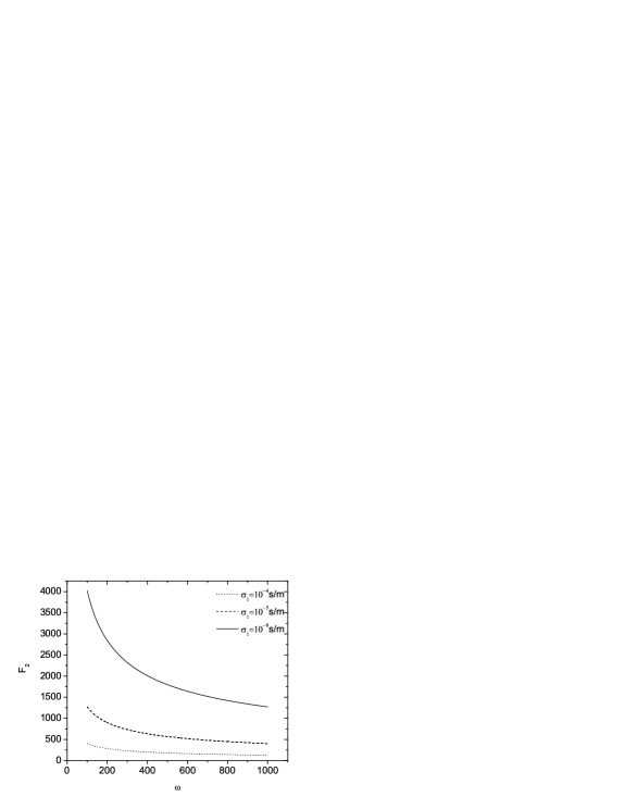
Figure 7: /Gao, Jian, Zhang, and Huang