Dynamics of tsunami waves

Abstract

The life of a tsunami is usually divided into three phases: the generation (tsunami source), the propagation and the inundation. Each phase is complex and often described separately. A brief description of each phase is given. Model problems are identified. Their formulation is given. While some of these problems can be solved analytically, most require numerical techniques. The inundation phase is less documented than the other phases. It is shown that methods based on Smoothed Particle Hydrodynamics (SPH) are particularly well-suited for the inundation phase. Directions for future research are outlined.

1 Introduction

Given the broadness of the topic of tsunamis, our purpose here is to recall some of the basics of tsunami modeling and to emphasize some general aspects, which are sometimes overlooked. The life of a tsunami is usually divided into three phases: the generation (tsunami source), the propagation and the inundation. The third and most difficult phase of the dynamics of tsunami waves deals with their breaking as they approach the shore. This phase depends greatly on the bottom bathymetry and on the coastline type. The breaking can be progressive. Then the inundation process is relatively slow and can last for several minutes. Structural damages are mainly caused by inundation. The breaking can also be explosive and lead to the formation of a plunging jet. The impact on the coast is then very rapid. In very shallow water, the amplitude of tsunami waves grows to such an extent that typically an undulation appears on the long wave, which develops into a progressive bore Chanson (2005). This turbulent front, similar to the wave that occurs when a dam breaks, can be quite high and travel onto the beach at great speed. Then the front and the turbulent current behind it move onto the shore, past buildings and vegetation until they are finally stopped by rising ground. The water level can rise rapidly, typically from 0 to 3 meters in 90 seconds.

The trajectory of these currents and their velocity are quite unpredictible, especially in the final stages because they are sensitive to small changes in the topography, and to the stochastic patterns of the collapse of buildings, and to the accumulation of debris such as trees, cars, logs, furniture. The dynamics of this final stage of tsunami waves is somewhat similar to the dynamics of flood waves caused by dam breaking, dyke breaking or overtopping of dykes (cf. the recent tragedy of hurricane Katrina in August 2005). Hence research on flooding events and measures to deal with them may be able to contribute to improved warning and damage reduction systems for tsunami waves in the areas of the world where these waves are likely to occur as shallow surge waves (cf. the recent tragedy of the Indian Ocean tsunami in December 2004).

Civil engineers who visited the damage area following the Boxing day tsunami came up with several basic conclusions. Buildings that had been constructed to satisfy modern safety standards offered a satisfactory resistance, in particular those with reinforced concrete beams properly integrated in the frame structure. These were able to withstand pressure associated with the leading front of the order of 1 atmosphere (recall that an equivalent pressure $p$ is obtained with a windspeed $U$ of about 450 m/s, since $p=\rho_{\rm air}U^{2}/2$). By contrast brick buildings collapsed and were washed away. Highly porous or open structures survived. Buildings further away from the beach survived the front in some cases, but they were then destroyed by the erosion of the ground around the buildings by the water currents Hunt and Burgers (2005).

Section 2 provides a description of the tsunami source when the source is an earthquake. In Section 3, we review the equations that are often used for tsunami propagation. Section 4 provides a short discussion on the energy of tsunamis. Section 5 is devoted to the run-up and inundation of tsunamis. Finally directions for future research are outlined.

2 Tsunami induced by near-shore earthquake

The inversion of seismic data allows one to reconstruct the permanent deformations of the sea bottom following earthquakes. In spite of the complexity of the seismic source and of the internal structure of the Earth, scientists have been relatively successful in using simple models for the source Okada (1985). A description of Okada’s model follows.

2.1 Introduction

The fracture zones, along which the foci of earthquakes are to be found, have been described in various papers. For example, it has been suggested that Volterra’s theory of dislocations might be the proper tool for a quantitative description of these fracture zones Steketee (1958). This suggestion was made for the following reason. If the mechanism involved in earthquakes and the fracture zones is indeed one of fracture, discontinuities in the displacement components across the fractured surface will exist. As dislocation theory may be described as that part of the theory of elasticity dealing with surfaces across which the displacement field is discontinuous, the suggestion seems reasonable.

As commonly done in mathematical physics, it is necessary for simplicity’s sake to make some assumptions. Here we neglect the curvature of the earth, its gravity, temperature, magnetism, non-homogeneity, and consider a semi-infinite medium, which is homogeneous and isotropic. We further assume that the laws of classical linear elasticity theory hold.

Several studies showed that the effect of earth curvature is negligible for shallow events at distances of less than $20^{\circ}$ McGinley (1969); Ben-Menahem et al. (1969); Ben-Mehanem et al. (1970); Smylie and Mansinha (1971). The sensitivity to earth topography, homogeneity, isotropy and half-space assumptions was studied and discussed recently Masterlark (2003). The author used a commercially available code, ABACUS, which is based on a finite element model (FEM). Six FEMs were constructed to test the sensitivity of deformation predictions to each assumption. The main conclusion is that the vertical layering of lateral inhomogeneity can sometimes cause considerable effects on the deformation fields.

The usual boundary conditions for dealing with earth’s problems require that the surface $S$ of the elastic medium (the earth) shall be free from forces. The resulting mixed boundary-value problem was solved a century ago Volterra (1907). Later, Steketee proposed an alternative method to solve this problem using Green’s functions Steketee (1958).

2.2 Volterra’s theory of dislocations

In order to introduce the concept of dislocation and for simplicity’s sake, this section is devoted to the case of an entire elastic space. The second reason is that in his original paper Volterra solved the problem in this case Volterra (1907).

Let $O$ be the origin of a Cartesian coordinate system in an infinite elastic medium, $x_{i}$ the Cartesian coordinates $(i=1,2,3)$, and $\mathbf{e}_{i}$ a unit vector in the positive $x_{i}$-direction. A force $\mathbf{F}=F\mathbf{e}_{k}$ at $O$ generates a displacement field $u_{i}^{k}(P,O)$ at point $P$, which is determined by the well-known Somigliana tensor

$$u_{i}^{k}(P,O)=\frac{F}{8\pi\mu}(\delta_{ik}r_{,\>nn}-\alpha r_{,\>ik}),\quad\mbox{with}\;\;\alpha=\frac{\lambda+\mu}{\lambda+2\mu}.$$ (1)

In this relation $\delta_{ik}$ is the Kronecker delta, $\lambda$ and $\mu$ are Lamé’s constants, and $r$ is the distance from $P$ to $O$. The coefficient $\alpha$ can be rewritten as $\alpha=1/2(1-\nu)$, where $\nu$ is Poisson’s ratio. Later we will also use Young’s modulus $E$, which is defined as

$$E=\frac{\mu\,(3\lambda+2\mu)}{\lambda+\mu}.$$

The notation $r_{,\>i}$ means $\partial r/\partial x_{i}$ and the summation convention applies.

The stresses due to the displacement field (1) are easily computed from Hooke’s law:

$$\sigma_{ij}=\lambda\delta_{ij}u_{k,k}+\mu(u_{i,j}+u_{j,i}).$$ (2)

We find

$$\sigma_{ij}^{k}(P,O)=-\frac{\alpha F}{4\pi}\left(3\frac{x_{i}x_{j}x_{k}}{r^{5}}+\frac{\mu}{\lambda+\mu}\frac{\delta_{ki}x_{j}+\delta_{kj}x_{i}-\delta_{ij}x_{k}}{r^{3}}\right).$$

The components of the force per unit area on a surface element are denoted as follows:

$$T_{i}^{k}=\sigma_{ij}^{k}\cdot\nu_{j},$$

where the $\nu_{j}$’s are the direction cosines of the normal to the surface element Sokolnikoff and Specht (1946). A Volterra dislocation is defined as a surface $\Sigma$ in the elastic medium across which there is a discontinuity $\Delta u_{i}$ in the displacement fields of the type

$$\Delta u_{i} = u_{i}^{+}-u_{i}^{-}=U_{i}+\Omega_{ij}x_{j},$$ (3)

$$\Omega_{ij} = -\Omega_{ji}.$$ (4)

Equation (3) in which $U_{i}$ and $\Omega_{ij}$ are constants is the well-known Weingarten relation which states that the discontinuity $\Delta u_{i}$ should be of the type of a rigid body displacement, thereby maintaining continuity of the components of stress and strain across $\Sigma$.

The displacement field in an infinite elastic medium due to a dislocation of type (1) is then determined by Volterra’s formula Volterra (1907)

$$u_{k}(y_{1},y_{2},y_{3}):=u_{k}(y_{l})=\frac{1}{F}\int\!\!\!\!\int\limits_{\!\!\!\!\!\!\!\Sigma}\Delta u_{i}T_{i}^{k}dS.$$ (5)

Once the surface $\Sigma$ is given, the dislocation is essentially determined by the six constants $U_{i}$ and $\Omega_{ij}$. Therefore we also write

$$u_{k}(y_{l})=\frac{U_{i}}{F}\int\!\!\!\!\int\limits_{\!\!\!\!\!\!\!\Sigma}\sigma_{ij}^{k}(P,Q)\nu_{j}dS+\frac{\Omega_{ij}}{F}\int\!\!\!\!\int\limits_{\!\!\!\!\!\!\!\Sigma}\{x_{j}\sigma_{il}^{k}(P,Q)-x_{i}\sigma_{jl}^{k}(P,Q)\}\nu_{l}dS,$$ (6)

where $\Omega_{ij}$ takes only the values $\Omega_{12}$, $\Omega_{23}$, $\Omega_{31}$. Following Volterra Volterra (1907) and Love Love (1944) we call each of the six integrals in (6) an elementary dislocation.

It is clear from (5) and (6) that the computation of the displacement field $u_{k}(Q)$ is performed as follows: A force $F\mathbf{e}_{k}$ is applied at $Q$, and the stresses $\sigma_{ij}^{k}(P,Q)$ that this force generates are computed at the points $P(x_{i})$ on $\Sigma$. In particular the components of the force on $\Sigma$ are computed. After multiplication with prescribed weights of magnitude $\Delta u_{i}$ these forces are integrated over $\Sigma$ to give the displacement component in $Q$ due to the dislocation on $\Sigma$.

2.3 Dislocations in elastic half-space

When the case of an elastic half-space is considered, equation (5) remains valid, but we have to replace $\sigma_{ij}^{k}$ by another tensor $\omega_{ij}^{k}$. This can be explained by the fact that the elementary solutions for a half-space are different from Somigliana solution (1).

The $\omega_{ij}^{k}$ can be obtained from the displacements corresponding to nuclei of strain in a half-space through relation (2). Steketee showed a method of obtaining the six $\omega_{ij}^{k}$ fields by using a Green’s function and derived $\omega_{12}^{k}$, which is relevant to a vertical strike-slip fault. Maruyama derived the remaining five functions Maruyama (1964).

It is interesting to mention here that historically these solutions were first derived in a straightforward manner by Mindlin Mindlin (1936); Mindlin and Cheng (1950), who gave explicit expressions of the displacement and stress fields for half-space nuclei of strain consisting of single forces with and without moment. It is only necessary to write the single force results since the other forms can be obtained by taking appropriate derivatives. Their method consists in finding the displacement field in Westergaard’s form of the Galerkin vector Westergaard (1935). This vector is then determined by taking a linear combination of some biharmonic elementary solutions. The coefficients are chosen to satisfy boundary and equilibrium conditions. These solutions were also derived by Press in a slightly different manner Press (1965).

Figure 1: Coordinate system adopted in this study and geometry of the source model

Here, we take the Cartesian coordinate system shown in Figure 1. The elastic medium occupies the region $z\leq 0$ and the $x-$axis is taken to be parallel to the strike direction of the fault. In this coordinate system, $u_{i}^{j}(x_{1},x_{2},x_{3};\xi_{1},\xi_{2},\xi_{3})$ is the $i$th component of the displacement at $(x_{1},x_{2},x_{3})$ due to the $j$th direction point force of magnitude $F$ at $(\xi_{1},\xi_{2},\xi_{3})$. It can be expressed as follows Mindlin (1936); Press (1965); Okada (1985, 1992):

$$u_{i}^{j}(x_{1},x_{2},x_{3})=u_{iA}^{j}(x_{1},x_{2},-x_{3})-u_{iA}^{j}(x_{1},x_{2},x_{3})+u_{iB}^{j}(x_{1},x_{2},x_{3})+x_{3}u_{iC}^{j}(x_{1},x_{2},x_{3}),$$ (7)

where

$$u_{iA}^{j} = \frac{F}{8\pi\mu}\left((2-\alpha)\frac{\delta_{ij}}{R}+\alpha\frac{R_{i}R_{j}}{R^{3}}\right),$$

$$u_{iB}^{j} = \frac{F}{4\pi\mu}\Biggl{(}\frac{\delta_{ij}}{R}+\frac{R_{i}R_{j}}{R^{3}}+\frac{1-\alpha}{\alpha}\Bigl{[}\frac{\delta_{ij}}{R+R_{3}}+$$

$$+\frac{R_{i}\delta_{j3}-R_{j}\delta_{i3}(1-\delta_{j3})}{R(R+R_{3})}-\frac{R_{i}R_{j}}{R(R+R_{3})^{2}}(1-\delta_{i3})(1-\delta_{j3})\Bigr{]}\Biggr{)},$$

$$u_{iC}^{j} = \frac{F}{4\pi\mu}(1-2\delta_{i3})\left((2-\alpha)\frac{R_{i}\delta_{j3}-R_{j}\delta_{i3}}{R^{3}}+\alpha\xi_{3}\left[\frac{\delta_{ij}}{R^{3}}-3\frac{R_{i}R_{j}}{R^{5}}\right]\right).$$

In these expressions $R_{1}=x_{1}-\xi_{1}$, $R_{2}=x_{2}-\xi_{2}$, $R_{3}=x_{3}-\xi_{3}$, $R^{2}=R_{1}^{2}+R_{2}^{2}+R_{3}^{2}$.

The first term in equation (7), $u_{iA}^{j}(x_{1},x_{2},x_{3})$, is the well-known Somigliana tensor, which represents the displacement field due to a single force placed at $(\xi_{1},\xi_{2},\xi_{3})$ in an infinite medium Love (1944). The second term also looks like a Somigliana tensor. This term corresponds to a contribution from an image source of the given point force placed at $(\xi_{1},\xi_{2},-\xi_{3})$ in the infinite medium. The third term, $u_{iB}^{j}(x_{1},x_{2},x_{3})$, and $u_{iC}^{j}(x_{1},x_{2},x_{3})$ in the fourth term are naturally depth dependent. When $x_{3}$ is set equal to zero in equation (7), the first and the second terms cancel each other, and the fourth term vanishes. The remaining term, $u_{iB}^{j}(x_{1},x_{2},0)$ reduces to the formula for the surface displacement field due to a point force in a half-space Okada (1985):

$$\left\{\begin{array}[]{ll}u_{1}^{1}=\frac{F}{4\pi\mu}\left(\frac{1}{R}+\frac{(x_{1}-\xi_{1})^{2}}{R^{3}}+\frac{\mu}{\lambda+\mu}\left[\frac{1}{R-\xi_{3}}-\frac{(x_{1}-\xi_{1})^{2}}{R(R-\xi_{3})^{2}}\right]\right),&\\ u_{2}^{1}=\frac{F}{4\pi\mu}(x_{1}-\xi_{1})(x_{2}-\xi_{2})\left(\frac{1}{R^{3}}-\frac{\mu}{\lambda+\mu}\frac{1}{R(R-\xi_{3})^{2}}\right),&\\ u_{3}^{1}=\frac{F}{4\pi\mu}(x_{1}-\xi_{1})\left(-\frac{\xi_{3}}{R^{3}}-\frac{\mu}{\lambda+\mu}\frac{1}{R(R-\xi_{3})}\right),&\end{array}\right.$$

$$\left\{\begin{array}[]{ll}u_{1}^{2}=\frac{F}{4\pi\mu}(x_{1}-\xi_{1})(x_{2}-\xi_{2})\left(\frac{1}{R^{3}}-\frac{\mu}{\lambda+\mu}\frac{1}{R(R-\xi_{3})^{2}}\right),&\\ u_{2}^{2}=\frac{F}{4\pi\mu}\left(\frac{1}{R}+\frac{(x_{2}-\xi_{2})^{2}}{R^{3}}+\frac{\mu}{\lambda+\mu}\left[\frac{1}{R-\xi_{3}}-\frac{(x_{2}-\xi_{2})^{2}}{R(R-\xi_{3})^{2}}\right]\right),&\\ u_{3}^{2}=\frac{F}{4\pi\mu}(x_{2}-\xi_{2})\left(-\frac{\xi_{3}}{R^{3}}-\frac{\mu}{\lambda+\mu}\frac{1}{R(R-\xi_{3})}\right),&\end{array}\right.$$

$$\left\{\begin{array}[]{ll}u_{1}^{3}=\frac{F}{4\pi\mu}(x_{1}-\xi_{1})\left(-\frac{\xi_{3}}{R^{3}}+\frac{\mu}{\lambda+\mu}\frac{1}{R(R-\xi_{3})}\right),&\\ u_{2}^{3}=\frac{F}{4\pi\mu}(x_{2}-\xi_{2})\left(-\frac{\xi_{3}}{R^{3}}+\frac{\mu}{\lambda+\mu}\frac{1}{R(R-\xi_{3})}\right),&\\ u_{3}^{3}=\frac{F}{4\pi\mu}\left(\frac{1}{R}+\frac{\xi_{3}^{2}}{R^{3}}+\frac{\mu}{\lambda+\mu}\frac{1}{R}\right).&\end{array}\right.$$

In these formulas $R^{2}=(x_{1}-\xi_{1})^{2}+(x_{2}-\xi_{2})^{2}+\xi_{3}^{2}$.

In order to obtain the displacements due to the dislocation we need to calculate the corresponding $\xi_{k}$-derivatives of the point force solution (7) and to put it in Steketee-Volterra formula (5)

$$u_{i}=\frac{1}{F}\int\!\!\!\!\int\limits_{\!\!\!\!\!\!\!\Sigma}\Delta u_{j}\left[\lambda\delta_{jk}\frac{\partial u_{i}^{n}}{\partial\xi_{n}}+\mu\left(\frac{\partial u_{i}^{j}}{\partial\xi_{k}}+\frac{\partial u_{i}^{k}}{\partial\xi_{j}}\right)\right]\nu_{k}dS.$$

It is expressed as follows:

$$\frac{\partial u_{i}^{j}}{\partial\xi_{k}}(x_{1},x_{2},x_{3}) = \frac{\partial u_{iA}^{j}}{\partial\xi_{k}}(x_{1},x_{2},-x_{3})-\frac{\partial u_{iA}^{j}}{\partial\xi_{k}}(x_{1},x_{2},x_{3})+$$

$$+\frac{\partial u_{iB}^{j}}{\partial\xi_{k}}(x_{1},x_{2},x_{3})+x_{3}\frac{\partial u_{iC}^{j}}{\partial\xi_{k}}(x_{1},x_{2},x_{3}),$$

with

$$\frac{\partial u_{iA}^{j}}{\partial\xi_{k}} = \frac{F}{8\pi\mu}\left((2-\alpha)\frac{R_{k}}{R^{3}}\delta_{ij}-\alpha\frac{R_{i}\delta_{jk}+R_{j}\delta_{ik}}{R^{3}}+3\alpha\frac{R_{i}R_{j}R_{k}}{R^{5}}\right),$$

$$\frac{\partial u_{iB}^{j}}{\partial\xi_{k}} = \frac{F}{4\pi\mu}\left(-\frac{R_{i}\delta_{jk}+R_{j}\delta_{ik}-R_{k}\delta_{ij}}{R^{3}}+3\frac{R_{i}R_{j}R_{k}}{R^{5}}\right.+$$

$$+\frac{1-\alpha}{\alpha}\Bigl{[}\frac{\delta_{3k}R+R_{k}}{R(R+R_{3})^{2}}\delta_{ij}-\frac{\delta_{ik}\delta_{j3}-\delta_{jk}\delta_{i3}(1-\delta_{j3})}{R(R+R_{3})}+$$

$$+\bigl{(}R_{i}\delta_{j3}-R_{j}\delta_{i3}(1-\delta_{j3})\bigr{)}\frac{\delta_{3k}R^{2}+R_{k}(2R+R_{3})}{R^{3}(R+R_{3})^{2}}+$$

$$\left.+(1-\delta_{i3})(1-\delta_{j3})\bigl{(}\frac{R_{i}\delta_{jk}+R_{j}\delta_{ik}}{R(R+R_{3})^{2}}-R_{i}R_{j}\frac{2\delta_{3k}R^{2}+R_{k}(3R+R_{3})}{R^{3}(R+R_{3})^{3}}\bigr{)}\Bigr{]}\right),$$

$$\frac{\partial u_{iC}^{j}}{\partial\xi_{k}} = \frac{F}{4\pi\mu}(1-2\delta_{i3})\biggl{(}(2-\alpha)\Bigl{[}\frac{\delta_{jk}\delta_{i3}-\delta_{ik}\delta_{j3}}{R^{3}}+\frac{3R_{k}(R_{i}\delta_{j3}-R_{j}\delta_{i3})}{R^{5}}\Bigr{]}+$$

$$+\alpha\delta_{3k}\Bigl{[}\frac{\delta_{ij}}{R^{3}}-\frac{3R_{i}R_{j}}{R^{5}}\Bigr{]}+3\alpha\xi_{3}\Bigl{[}\frac{R_{i}\delta_{jk}+R_{j}\delta_{ik}+R_{k}\delta_{ij}}{R^{5}}-\frac{5R_{i}R_{j}R_{k}}{R^{7}}\Bigr{]}\biggr{)}.$$

2.4 Finite rectangular source

Now, let us consider a more practical problem. We define the elementary dislocations $U_{1}$, $U_{2}$, and $U_{3}$, corresponding to the strike-slip, dip-slip, and tensile components of an arbitrary dislocation. In Figure 1 each vector represents the direction of the elementary faults. The vector $\mathbf{D}$ is the so-called Burger’s vector, which shows how both sides of the fault are spread out: $\mathbf{D}=\mathbf{u}^{+}-\mathbf{u}^{-}$.

A general dislocation can be determined by three angles: the dip angle $\delta$ of the fault, the slip angle $\theta$, and the angle $\phi$ between the fault plane and Burger’s vector $\mathbf{D}$. This situation is schematically described in Figure 2.

Figure 2: Geometry of the source model and orientation of Burger’s vector $\mathbf{D}$

For a finite rectangular fault with length $L$ and width $W$ occurring at depth $d$ (Figure 2), the deformation field can be evaluated analytically by changing the variables and performing integration over the rectangle. This was done by several authors Chinnery (1963); Sato and Matsu’ura (1974); Iwasaki and Sato (1979); Okada (1985, 1992). Here we give the results of their computations. The final results represented in compact form are listed below using Chinnery’s notation $\|$ to represent the substitution

$$f(\xi,\eta)\|=f(x,p)-f(x,p-W)-f(x-L,p)+f(x-L,p-W).$$

Let us introduce the following notation:

$$p=y\cos\delta+d\sin\delta,\quad q=y\sin\delta-d\cos\delta,$$

$$\tilde{y}=\eta\cos\delta+q\sin\delta,\quad\tilde{d}=\eta\sin\delta-q\cos\delta,$$

$$R^{2}=\xi^{2}+\eta^{2}+q^{2}=\xi^{2}+\tilde{y}^{2}+\tilde{d}^{2},\quad X^{2}=\xi^{2}+q^{2}.$$

The quantities $U_{1}$, $U_{2}$ and $U_{3}$ are linked to Burger’s vector through the identities

$$U_{1}=|\mathbf{D}|\cos\phi\cos\theta,\quad U_{2}=|\mathbf{D}|\cos\phi\sin\theta,\quad U_{3}=|\mathbf{D}|\sin\phi.$$

For a strike-slip dislocation, one has

$$u_{1} = -\frac{U_{1}}{2\pi}\left.\left(\frac{\xi q}{R(R+\eta)}+\arctan\frac{\xi\eta}{qR}+I_{1}\sin\delta\right)\right\|,$$

$$u_{2} = -\frac{U_{1}}{2\pi}\left.\left(\frac{\tilde{y}q}{R(R+\eta)}+\frac{q\cos\delta}{R+\eta}+I_{2}\sin\delta\right)\right\|,$$

$$u_{3} = -\frac{U_{1}}{2\pi}\left.\left(\frac{\tilde{d}q}{R(R+\eta)}+\frac{q\sin\delta}{R+\eta}+I_{4}\sin\delta\right)\right\|.$$

For a dip-slip dislocation, one has

$$u_{1} = -\frac{U_{2}}{2\pi}\left.\left(\frac{q}{R}-I_{3}\sin\delta\cos\delta\right)\right\|,$$

$$u_{2} = -\frac{U_{2}}{2\pi}\left.\left(\frac{\tilde{y}q}{R(R+\xi)}+\cos\delta\arctan\frac{\xi\eta}{qR}-I_{1}\sin\delta\cos\delta\right)\right\|,$$

$$u_{3} = -\frac{U_{2}}{2\pi}\left.\left(\frac{\tilde{d}q}{R(R+\xi)}+\sin\delta\arctan\frac{\xi\eta}{qR}-I_{5}\sin\delta\cos\delta\right)\right\|.$$

For a tensile fault dislocation, one has

$$u_{1} = \frac{U_{3}}{2\pi}\left.\left(\frac{q^{2}}{R(R+\eta)}-I_{3}\sin^{2}\delta\right)\right\|,$$

$$u_{2} = \frac{U_{3}}{2\pi}\left.\left(\frac{-\tilde{d}q}{R(R+\xi)}-\sin\delta\left[\frac{\xi q}{R(R+\eta)}-\arctan\frac{\xi\eta}{qR}\right]-I_{1}\sin^{2}\delta\right)\right\|,$$

$$u_{3} = \frac{U_{3}}{2\pi}\left.\left(\frac{\tilde{y}q}{R(R+\xi)}+\cos\delta\left[\frac{\xi q}{R(R+\eta)}-\arctan\frac{\xi\eta}{qR}\right]-I_{5}\sin^{2}\delta\right)\right\|.$$

The terms $I_{1},\dots,I_{5}$ are given by

$$I_{1} = -\frac{\mu}{\lambda+\mu}\frac{\xi}{(R+\tilde{d})\cos\delta}-\tan\delta I_{5},$$

$$I_{2} = -\frac{\mu}{\lambda+\mu}\log(R+\eta)-I_{3},$$

$$I_{3} = \frac{\mu}{\lambda+\mu}\left[\frac{1}{\cos\delta}\frac{\tilde{y}}{R+\tilde{d}}-\log(R+\eta)\right]+\tan\delta I_{4},$$

$$I_{4} = \frac{\mu}{\mu+\lambda}\frac{1}{\cos\delta}\left(\log(R+\tilde{d})-\sin\delta\log(R+\eta)\right),$$

$$I_{5} = \frac{\mu}{\lambda+\mu}\frac{2}{\cos\delta}\arctan\frac{\eta(X+q\cos\delta)+X(R+X)\sin\delta}{\xi(R+X)\cos\delta},$$

and if $\cos\delta=0$,

$$I_{1} = -\frac{\mu}{2(\lambda+\mu)}\frac{\xi q}{(R+\tilde{d})^{2}},$$

$$I_{3} = \frac{\mu}{2(\lambda+\mu)}\left[\frac{\eta}{R+\tilde{d}}+\frac{\tilde{y}q}{(R+\tilde{d})^{2}}-\log(R+\eta)\right],$$

$$I_{4} = -\frac{\mu}{\lambda+\mu}\frac{q}{R+\tilde{d}},$$

$$I_{5} = -\frac{\mu}{\lambda+\mu}\frac{\xi\sin\delta}{R+\tilde{d}}.$$

Figures 3, 4, and 5 show the free-surface deformation after three elementary dislocations. The values of the parameters are given in Table 1.

parameter	value
Dip angle $\delta$	$13^{\circ}$
Fault depth $d$, km	25
Fault length $L$, km	220
Fault width $W$, km	90
$U_{i}$, m	30
Young modulus $E$, GPa	9.5
Poisson’s ratio $\nu$	0.23

Table 1: Parameter set used in Figures 3, 4, and 5.

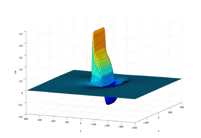
Figure 3: Dimensionless free-surface deformation $z/a$ after dip-slip fault. Here $a$ is $|\mathbf{D}|$ (30 m in the present application).

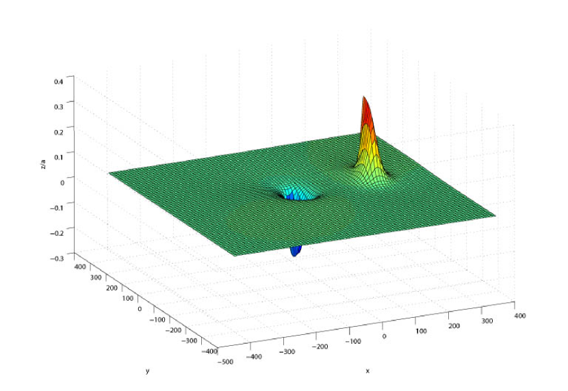
Figure 4: Dimensionless free-surface deformation $z/a$ after strike-slip fault. Here $a$ is $|\mathbf{D}|$ (30 m in the present application).

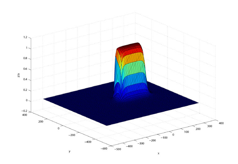
Figure 5: Dimensionless free-surface deformation $z/a$ after tensile fault. Here $\mathbf{D}=(0,0,U_{3})$ and $a=U_{3}$.

The traditional approach for hydrodynamic modelers is indeed to use elastic models similar to the model just described with the seismic parameters as input to evaluate details of the seafloor deformation. Then this deformation is translated to the initial condition of the evolution problem described in the next section. A few authors have solved the linearized water wave equations in the presence of a moving bottom Hammack (1973); Todorovska and Trifunac (2001).

3 Propagation of tsunamis

The problem of tsunami propagation is a special case of the general water-wave problem. The study of water waves relies on several common assumptions. Some are obvious while some others are questionable under certain circumstances. The water is assumed to be incompressible. Dissipation is not often included. However there are three main sources of dissipation for water waves: bottom friction, surface dissipation and body dissipation. For tsunamis, bottom friction is the most important one, especially in the later stages, and is sometimes included in the computations in an ad-hoc way. In most theoretical analyses, it is not included.

A brief description of the common mathematical model used to study water waves follows. The horizontal coordinates are denoted by $x$ and $y$, and the vertical coordinate by $z$. The horizontal gradient is denoted by

$$\nabla:=\left(\frac{\partial}{\partial x},\frac{\partial}{\partial y}\right).$$

The horizontal velocity is denoted by

$$\mathbf{u}(x,y,z,t)=(u,v)$$

and the vertical velocity by $w(x,y,z,t)$. The three-dimensional flow of an inviscid and incompressible fluid is governed by the conservation of mass

$$\nabla\cdot\mathbf{u}+\frac{\partial w}{\partial z}=0$$ (8)

and by the conservation of momentum

$$\rho\frac{{\rm D}\mathbf{u}}{{\rm D}t}=-\nabla p,\quad\rho\frac{{\rm D}w}{{\rm D}t}=-\rho g-\frac{\partial p}{\partial z}.$$ (9)

In (9), $\rho$ is the density of water (assumed to be constant throughout the fluid domain), $g$ is the acceleration due to gravity and $p(x,y,z,t)$ the pressure field.

The assumption that the flow is irrotational is commonly made to analyze surface waves. Then there exists a scalar function $\phi(x,y,z,t)$ (the velocity potential) such that

$$\mathbf{u}=\nabla\phi,\quad w=\frac{\partial\phi}{\partial z}.$$

The continuity equation (8) becomes

$$\nabla^{2}\phi+\frac{\partial^{2}\phi}{\partial z^{2}}=0\,.$$ (10)

The equation of momentum conservation (9) can be integrated into Bernoulli’s equation

$$\frac{\partial\phi}{\partial t}+\frac{1}{2}|\nabla\phi|^{2}+\frac{1}{2}\left(\frac{\partial\phi}{\partial z}\right)^{2}+gz+\frac{p-p_{0}}{\rho}=0\,,$$ (11)

which is valid everywhere in the fluid. The constant $p_{0}$ is a pressure of reference, for example the atmospheric pressure. The effects of surface tension are not important for tsunami propagation.

3.1 Classical formulation

The surface wave problem consists in solving Laplace’s equation (10) in a domain $\Omega(t)$ bounded above by a moving free surface (the interface between air and water) and below by a fixed solid boundary (the bottom). The free surface is represented by $F(x,y,z,t):=\eta(x,y,t)-z=0$. The shape of the bottom is given by $z=-h(x,y)$. The main driving force is gravity.

The free surface must be found as part of the solution. Two boundary conditions are required. The first one is the kinematic condition. It can be stated as ${\rm D}F/{\rm D}t=0$ (the material derivative of $F$ vanishes), which leads to

$$\eta_{t}+\nabla\phi\cdot\nabla\eta-\phi_{z}=0\quad\mbox{at}\;\;z=\eta(x,y,t)\,.$$ (12)

The second boundary condition is the dynamic condition which states that the normal stresses must be in balance at the free surface. The normal stress at the free surface is given by the difference in pressure. Bernoulli’s equation (11) evaluated on the free surface $z=\eta$ gives

$$\phi_{t}+\hbox{$\frac{1}{2}$}|\nabla\phi|^{2}+\hbox{$\frac{1}{2}$}\phi_{z}^{2}+g\eta=0\quad\mbox{at}\;\;z=\eta(x,y,t)\,.$$ (13)

Finally, the boundary condition at the bottom is

$$\nabla\phi\cdot\nabla h+\phi_{z}=0\quad\mbox{at}\;\;z=-h(x,y)\,.$$ (14)

To summarize, the goal is to solve the set of equations (10), (12), (13) and (14) for $\eta(x,y,t)$ and $\phi(x,y,z,t)$. When the initial value problem is integrated, the fields $\eta(x,y,0)$ and $\phi(x,y,z,0)$ must be specified at $t=0$. The conservation of momentum equation (9) is not required in the solution procedure; it is used a posteriori to find the pressure $p$ once $\eta$ and $\phi$ have been found.

In the following subsections, we will consider various approximations of the full water-wave equations. One is the system of Boussinesq equations, that retains nonlinearity and dispersion up to a certain order. Another one is the system of nonlinear shallow-water equations that retains nonlinearity but no dispersion. The simplest one is the system of linear shallow-water equations. The concept of shallow water is based on the smallness of the ratio between water depth and wave length. In the case of tsunamis propagating on the surface of deep oceans, one can consider that shallow-water theory is appropriate because the water depth (typically several kilometers) is much smaller than the wave length (typically several hundred kilometers).

3.2 Dimensionless formulation

The derivation of shallow-water type equations is a classical topic. Two dimensionless numbers, which are supposed to be small, are introduced:

$$\alpha=\frac{a}{d}\ll 1,\quad\beta=\frac{d^{2}}{\ell^{2}}\ll 1,$$ (15)

where $d$ is a typical water depth, $a$ a typical wave amplitude and $\ell$ a typical wavelength. The assumptions on the smallness of these two numbers are satisfied for the Indian Ocean tsunami. Indeed the satellite altimetry observations of the tsunami waves obtained by two satellites that passed over the Indian Ocean a couple of hours after the rupture occurred give an amplitude $a$ of roughly 60 cm in the open ocean. The typical wavelength estimated from the width of the segments that experienced slip is between 160 and 240 km Lay et al. (2005). The water depth ranges from 4 km towards the west of the rupture to 1 km towards the east. These values give the following ranges for the two dimensionless numbers:

$$1.5\times 10^{-4}<\alpha<6\times 10^{-4},\quad 1.7\times 10^{-5}<\beta<6.25\times 10^{-4}.$$ (16)

The equations are more transparent when written in dimensionless variables. The new independent variables are

$$x=\ell\tilde{x},\quad y=\ell\tilde{y},\quad z=d\tilde{z},\quad t=\ell\tilde{t}/c_{0},$$ (17)

where $c_{0}=\sqrt{gd}$, the famous speed of propagation of tsunamis in the open ocean ranging from 356 km/h for a 1 km water depth to 712 km/h for a 4 km water depth. The new dependent variables are

$$\eta=a\tilde{\eta},\quad h=d\tilde{h},\quad\phi=ga\ell\tilde{\phi}/c_{0}.$$ (18)

In dimensionless form, and after dropping the tildes, the equations become

$$\beta\nabla^{2}\phi+\phi_{zz} = 0,$$ (19)

$$\beta\nabla\phi\cdot\nabla h+\phi_{z} = 0\quad\mbox{at}\;\;z=-h(x,y),$$ (20)

$$\beta\eta_{t}+\alpha\beta\nabla\phi\cdot\nabla\eta = \phi_{z}\quad\mbox{at}\;\;z=\alpha\eta(x,y,t),$$ (21)

$$\beta\phi_{t}+\hbox{$\frac{1}{2}$}\alpha\beta|\nabla\phi|^{2}+\hbox{$\frac{1}{2}$}\alpha\phi_{z}^{2}+\beta\eta = 0\quad\mbox{at}\;\;z=\alpha\eta(x,y,t).$$ (22)

So far, no approximation has been made. In particular, we have not used the fact that the numbers $\alpha$ and $\beta$ are small.

3.3 Shallow-water equations

When $\beta$ is small, the water is considered to be shallow. The linearized theory of water waves is recovered by letting $\alpha$ go to zero. For the shallow water-wave theory, one assumes that $\beta$ is small and expand $\phi$ in terms of $\beta$:

$$\phi=\phi_{0}+\beta\phi_{1}+\beta^{2}\phi_{2}+\cdots.$$

This expansion is substituted into the governing equation and the boundary conditions. The lowest-order term in Laplace’s equation is

$$\phi_{0zz}=0.$$ (23)

The boundary conditions imply that $\phi_{0}=\phi_{0}(x,y,t)$. Thus the vertical velocity component is zero and the horizontal velocity components are independent of the vertical coordinate $z$ at lowest order. Let $\phi_{0x}=u(x,y,t)$ and $\phi_{0y}=v(x,y,t)$. Assume now for simplicity that the water depth is constant ($h=1$). Solving Laplace’s equation and taking into account the bottom kinematic condition yields the following expressions for $\phi_{1}$ and $\phi_{2}$:

$$\phi_{1}(x,y,z,t) = -\hbox{$\frac{1}{2}$}(1+z)^{2}(u_{x}+v_{y}),$$ (24)

$$\phi_{2}(x,y,z,t) = \hbox{$\frac{1}{24}$}(1+z)^{4}[(\nabla^{2}u)_{x}+(\nabla^{2}v)_{y}].$$ (25)

The next step consists in retaining terms of requested order in the free-surface boundary conditions. Powers of $\alpha$ will appear when expanding in Taylor series the free-surface conditions around $z=0$. For example, if one keeps terms of order $\alpha\beta$ and $\beta^{2}$ in the dynamic boundary condition (22) and in the kinematic boundary condition (21), one obtains

$$\beta\phi_{0t}-\hbox{$\frac{1}{2}$}\beta^{2}(u_{tx}+v_{ty})+\beta\eta+\hbox{$\frac{1}{2}$}\alpha\beta(u^{2}+v^{2}) = 0,$$ (26)

$$\beta[\eta_{t}+\alpha(u\eta_{x}+v\eta_{y})+(1+\alpha\eta)(u_{x}+v_{y})] = \hbox{$\frac{1}{6}$}\beta^{2}[(\nabla^{2}u)_{x}+(\nabla^{2}v)_{y}].$$ (27)

Differentiating (26) first with respect to $x$ and then to respect to $y$ gives a set of two equations:

$$u_{t}+\alpha(uu_{x}+vv_{x})+\eta_{x}-\hbox{$\frac{1}{2}$}\beta(u_{txx}+v_{txy}) = 0,$$ (28)

$$v_{t}+\alpha(uu_{y}+vv_{y})+\eta_{y}-\hbox{$\frac{1}{2}$}\beta(u_{txy}+v_{tyy}) = 0.$$ (29)

The kinematic condition (27) can be rewritten as

$$\eta_{t}+[u(1+\alpha\eta)]_{x}+[v(1+\alpha\eta)]_{y}=\hbox{$\frac{1}{6}$}\beta[(\nabla^{2}u)_{x}+(\nabla^{2}v)_{y}].$$ (30)

Equations (28)–(30) contain in fact various shallow-water models. The so-called fundamental shallow-water equations are obtained by neglecting the terms of order $\beta$:

$$u_{t}+\alpha(uu_{x}+vu_{y})+\eta_{x} = 0,$$ (31)

$$v_{t}+\alpha(uv_{x}+vv_{y})+\eta_{y} = 0,$$ (32)

$$\eta_{t}+[u(1+\alpha\eta)]_{x}+[v(1+\alpha\eta)]_{y} = 0.$$ (33)

Recall that we assumed $h$ to be constant for the derivation. Going back to an arbitrary water depth and to dimensional variables, the system of nonlinear shallow water equations reads

$$u_{t}+uu_{x}+vu_{y}+g\eta_{x} = 0,$$ (34)

$$v_{t}+uv_{x}+vv_{y}+g\eta_{y} = 0,$$ (35)

$$\eta_{t}+[u(h+\eta)]_{x}+[v(h+\eta)]_{y} = 0.$$ (36)

This system of equations has been used for example by Titov and Synolakis for the numerical computation of tidal wave run-up Titov and Synolakis (1998). Note that this model does not include any bottom friction terms. To solve the problem of tsunami generation caused by bottom displacement, the motion of the seafloor obtained from seismological models Okada (1985) and described in Section 3 can be prescribed during a time $t_{0}$. Usually $t_{0}$ is assumed to be small, so that the bottom displacement is considered as an instantaneous vertical displacement. This assumption may not be appropriate for slow events.

The satellite altimetry observations of the Indian Ocean tsunami clearly show dispersive effects. The question of dispersive effects in tsunamis is open. Most propagation codes ignore dispersion. A few propagation codes that include dispersion have been developed Dalrymple et al. (2006). A well-known code is FUNWAVE, developed at the University of Delaware over the past ten years Kirby et al. (1998). Dispersive shallow water-wave models are presented next.

3.4 Boussinesq equations

An additional dimensionless number, sometimes called the Stokes number, is introduced:

$$S=\frac{\alpha}{\beta}\approx 1.$$ (37)

For the Indian Ocean tsunami, one finds

$$0.24<S<46.$$ (38)

Therefore the additional assumption that $S\approx 1$ may be realistic.

In this subsection, we provide the guidelines to derive Boussinesq-type systems of equations Bona et al. (2002). Of course, the variation of bathymetry is essential for the propagation of tsunamis, but for the derivation the water depth will be assumed to be constant. Some notation is introduced. The potential evaluated along the free surface is denoted by $\Phi(x,y,t):=\phi(x,y,\eta,t)$. The derivatives of the velocity potential evaluated on the free surface are denoted by $\Phi_{(*)}(x,y,t):=\phi_{*}(x,y,\eta,t),$ where the star stands for $x$, $y$, $z$ or $t$. Consequently, $\Phi_{*}$ (defined for $*\neq z$) and $\Phi_{(*)}$ have different meanings. They are however related since

$$\Phi_{*}=\Phi_{(*)}+\Phi_{(z)}\eta_{*}\,.$$

The vertical velocity at the free surface is denoted by $W(x,y,t):=\phi_{z}(x,y,\eta,t)$.

The boundary conditions on the free surface (12) and (13) become

$$\eta_{t}+\nabla\Phi\cdot\nabla\eta-W(1+\nabla\eta\cdot\nabla\eta) = 0,$$ (39)

$$\Phi_{t}+g\eta+\hbox{$\frac{1}{2}$}|\nabla\Phi|^{2}-\hbox{$\frac{1}{2}$}W^{2}(1+\nabla\eta\cdot\nabla\eta) = 0.$$ (40)

These two nonlinear equations provide time-stepping for $\eta$ and $\Phi$. In addition, Laplace’s equation as well as the kinematic condition on the bottom must be satisfied. In order to relate the free-surface variables with the bottom variables, one must solve Laplace’s equation in the whole water column. In Boussinesq-type models, the velocity potential is represented as a formal expansion,

$$\phi(x,y,z,t)=\sum_{n=0}^{\infty}\phi^{(n)}(x,y,t)\,z^{n}.$$ (41)

Here the expansion is about $z=0$, which is the location of the free surface at rest. Demanding that $\phi$ formally satisfy Laplace’s equation leads to a recurrence relation between $\phi^{(n)}$ and $\phi^{(n+2)}$. Let $\phi_{o}$ denote the velocity potential at $z=0$, $\mathbf{u}_{o}$ the horizontal velocity at $z=0$, and $w_{o}$ the vertical velocity at $z=0$. Note that $\phi_{o}$ and $w_{o}$ are nothing else than $\phi^{(0)}$ and $\phi^{(1)}$. The potential $\phi$ can be expressed in terms of $\phi_{o}$ and $w_{o}$ only. Finally, one obtains the velocity field in the whole water column $(-h\leq z\leq\eta)$ Madsen et al. (2003):

$$\mathbf{u}(x,y,z,t) = \cos(z\nabla)\mathbf{u}_{o}+\sin(z\nabla)w_{o},$$ (42)

$$w(x,y,z,t) = \cos(z\nabla)w_{o}-\sin(z\nabla)\mathbf{u}_{o}.$$ (43)

Here the cosine and sine operators are infinite Taylor series operators defined by

$$\cos(z\nabla)=\sum_{n=0}^{\infty}(-1)^{n}\frac{z^{2n}}{(2n)!}\nabla^{2n},\quad\sin(z\nabla)=\sum_{n=0}^{\infty}(-1)^{n}\frac{z^{2n+1}}{(2n+1)!}\nabla^{2n+1}.$$

Then one can substitute the representation (42)-(43) into the kinematic bottom condition and use successive approximations to obtain an explicit recursive expression for $w_{o}$ in terms of $\mathbf{u}_{o}$ to infinite order in $h\nabla$.

A wide variety of Boussinesq systems can been derived Madsen et al. (2003). One can generalize the expansions to an arbitrary $z-$level, instead of the $z=0$ level. The Taylor series for the cosine and sine operators can be truncated, Padé approximants can be used in operators at $z=-h$ and/or at $z=0$.

The classical Boussinesq equations are more transparent when written in the dimensionless variables used in the previous subsection. We further assume that $h$ is constant, drop the tildes, and write the equations for one spatial dimension ($x$). Performing the expansion about $z=0$ leads to the vanishing of the odd terms in the velocity potential. Substituting the expression for $\phi$ into the free-surface boundary conditions evaluated at $z=1+\alpha\eta(x,t)$ leads to two equations in $\eta$ and $\phi_{o}$ with terms of various order in $\alpha$ and $\beta$. The small parameters $\alpha$ and $\beta$ are of the same order, while $\eta$ and $\phi_{o}$ as well as their partial derivatives are of order one.

3.5 Classical Boussinesq equations

The classical Boussinesq equations are obtained by keeping all terms that are at most linear in $\alpha$ or $\beta$. In the derivation of the fundamental nonlinear shallow-water equations (31)–(33), the terms in $\beta$ were neglected. It is therefore implicitly assumed that the Stokes number is large. Since the cube of the water depth appears in the denominator of the Stokes number ($S=\alpha/\beta=a\ell^{2}/d^{3}$), it means that the Stokes number is 64 times larger in a 1 km depth than in a 4 km depth! Based on these arguments, dispersion is more important to the west of the rupture. Considering the Stokes number to be of order one leads to the following system in dimensional form:

$$u_{t}+uu_{x}+g\eta_{x}-\hbox{$\frac{1}{2}$}h^{2}u_{txx} = 0,$$ (44)

$$\eta_{t}+[u(h+\eta)]_{x}-\hbox{$\frac{1}{6}$}h^{3}u_{xxx} = 0.$$ (45)

The classical Boussinesq equations are in fact slightly different. They are obtained by replacing $u$ with the depth averaged velocity

$$\frac{1}{h}\int_{-h}^{\eta}u\,dz.$$

They read

$$u_{t}+uu_{x}+g\eta_{x}-\hbox{$\frac{1}{3}$}h^{2}u_{txx} = 0,$$ (46)

$$\eta_{t}+[u(h+\eta)]_{x} = 0.$$ (47)

A number of variants of the classical Boussinesq system were studied by Bona et al., who in particular showed that depending on the modeling of dispersion the linearization about the rest state may or may not be well-posed Bona et al. (2002).

3.6 Korteweg–de Vries equation

The previous system allows the propagation of waves in both the positive and negative $x-$directions. Seeking solutions travelling in only one direction, for example the positive $x-$direction, leads to a single equation for $\eta$, the Korteweg–de Vries equation:

$$\eta_{t}+c_{0}\left(1+\frac{3\eta}{2d}\right)\eta_{x}+\frac{1}{6}c_{0}d^{2}\eta_{xxx}=0,$$ (48)

where $d$ is the water depth. It admits solitary wave solutions travelling at speed $V$ in the form

$$\eta(x,t)=a\,\mbox{sech}^{2}\left(\sqrt{\frac{3a}{4d^{3}}}(x-Vt)\right),\quad\mbox{with}\;\;V=c_{0}\left(1+\frac{a}{2d}\right).$$

The solitary wave solutions of the Korteweg–de Vries equation are of elevation ($a>0$) and travel faster than $c_{0}$. Their speed increases with amplitude. Note that a natural length scale appears:

$$\ell=\sqrt{\frac{4d^{3}}{3a}}.$$

For the Indian Ocean tsunami, it gives roughly $\ell=377$ km. It is of the order of magnitude of the wavelength estimated from the width of the segments that experienced slip.

4 Energy of a tsunami

The energy of the earthquake is measured via the strain energy released by the faulting. The part of the energy transmitted to the tsunami wave is less than one percent Lay et al. (2005). They estimate the tsunami energy to be $4.2\times 10^{15}$ J. They do not give details on how they obtained this estimate. However, a simple calculation based on considering the tsunami as a soliton

$$\eta(x)=a\,\mbox{sech}^{2}\left(\frac{x}{\ell}\right),\quad u(x)=\alpha c_{0}\,\mbox{sech}^{2}\left(\frac{x}{\ell}\right),$$

gives for the energy

$$E=\frac{1}{\sqrt{3}}\alpha^{3/2}\rho d^{2}(c_{0}^{2}+gd)\int_{-\infty}^{\infty}\mbox{sech}^{4}x\,dx+O(\alpha^{2}).$$

The value for the integral is $4/3$. The numerical estimate for $E$ is close to that of Lay et al. (2005). Incidently, at this level of approximation, there is equipartition between kinetic and potential energy. It is also important to point out that a tsunami being a shallow water wave, the whole water column is moving as the wave propagates. For the parameter values used so far, the maximum horizontal current is 3 cm/s. However, as the water depth decreases, the current increases and becomes important when the depth becomes less than 500 m. Additional properties of solitary waves can be found for example in Longuet-Higgins (1974).

5 Tsunami run-up

The last phase of a tsunami is its run-up and inundation. Although in some cases it may be important to consider the coupling between fluid and structures, we restrict ourselves to the description of the fluid flow. The problem of waves climbing a beach is a classical one Carrier and Greenspan (1958). The transformations used by Carrier and Greenspan are still used nowadays. The basis of their analysis is the one-dimensional counterpart of the system (34)–(36). In addition, they assume the depth to be of uniform slope: $h=-x\tan\theta$. Introduce the following dimensionless quantities, where $\ell$ is a characteristic length:

$$x=\ell\tilde{x},\;\;\eta=\ell\tilde{\eta},\;\;u=\sqrt{g\ell}\,\tilde{u},\;\;t=\sqrt{\ell/g}\,\tilde{t},\;\;c^{2}=(h+\eta)/\ell.$$

After dropping the tildes, the dimensionless system of equations (34)-(36) becomes

$$u_{t}+uu_{x}+\eta_{x} = 0,$$

$$\eta_{t}+[u(-x\tan\theta+\eta)]_{x} = 0.$$

In terms of the variable $c$, these equations become

$$u_{t}+uu_{x}+2cc_{x}+\tan\theta = 0,$$

$$2c_{t}+cu_{x}+2uc_{x} = 0.$$

The equations written in characteristic form are

$$\left[\frac{\partial}{\partial t}+(u+c)\frac{\partial}{\partial x}\right](u+2c+t\tan\theta) = 0,$$

$$\left[\frac{\partial}{\partial t}+(u-c)\frac{\partial}{\partial x}\right](u-2c+t\tan\theta) = 0.$$

The characteristic curves $C^{+}$ and $C^{-}$ as well as the Riemann invariants are

$$C^{+} : \frac{dx}{dt}=u+c,\quad u+2c+t\tan\theta=r,$$

$$C^{-} : \frac{dx}{dt}=u-c,\quad u-2c+t\tan\theta=s.$$

Next one can rewrite the hyperbolic equations in terms of the new variables $\lambda$ and $\sigma$ defined as follows:

$$\frac{\lambda}{2} = \frac{1}{2}(r+s)=u+t\tan\theta,$$

$$\frac{\sigma}{4} = \frac{1}{4}(r-s)=c.$$

One obtains

$$x_{s}-\left[\frac{1}{4}(3r+s)-t\tan\theta\right]t_{s} = 0,$$

$$x_{r}-\left[\frac{1}{4}(r+3s)-t\tan\theta\right]t_{r} = 0.$$

The elimination of $x$ results in the linear second-order equation for $t$

$$\sigma(t_{\lambda\lambda}-t_{\sigma\sigma})-3t_{\sigma}=0.$$ (49)

Since $u+t\tan\theta=\lambda/2$, $u$ must also satisfy (49). Introducing the potential $\phi(\sigma,\lambda)$ such that

$$u=\frac{\phi_{\sigma}}{\sigma},$$

one obtains the equation

$$(\sigma\phi_{\sigma})_{\sigma}-\sigma\phi_{\lambda\lambda}=0$$

after integrating once. Two major simplifications have been obtained. The nonlinear set of equations have been reduced to a linear equation for $u$ or $\phi$ and the free boundary is now the fixed line $\sigma=0$ in the $(\sigma,\lambda)-$plane. The free boundary is the instantaneous shoreline $c=0$, which moves as a wave climbs a beach.

The above formulation has been used by several authors to study the run-up of various types of waves on sloping beaches Tadepalli and Synolakis (1994); Carrier et al. (2003); Tinti and Tonini (2005). For example, it has been shown that leading depression $N$-waves run-up higher than leading elevation $N$-waves, suggesting that perhaps the solitary wave model may not be adequate for predicting an upper limit for the run-up of near-shore generated tsunamis.

There is a rule of thumb that says that the run-up does not usually exceed twice the fault slip. Since run-ups of 30 meters were observed in Sumatra during the Boxing Day tsunami, the slip might have been of 15 meters or even more.

Analytical models are useful, especially to perform parametric studies. However, the breaking of tsunami waves as well as the subsequent floodings must be studied numerically. The most natural methods that can be used are the free surface capturing methods based on a finite volume discretisation, such as the Volume Of Fluid (VOF) or the Level Set methods, and the family of Smoothed Particle Hydrodynamics methods (SPH), applied to free-surface flow problems Monaghan (1994); Gomez-Gesteira and Dalrymple (2004); Gomez-Gesteira et al. (2005). Such methods allow a study of flood wave dynamics, of wave breaking on the land behind beaches, and of the flow over rising ground with and without the presence of obstacles. This task is an essential part of tsunami modelling, since it allows the determination of the level of risk due to major flooding, the prediction of the resulting water levels in the flooded areas, the determination of security zones. It also provides some help in the conception and validation of protection systems in the most exposed areas.

6 Direction for future research

A useful direction for future research in the dynamics of tsunami waves is the three-dimensional (3D) simulation of tsunami breaking along a coast. For this purpose, different validation steps are necessary. First more simulations of a two-dimensional (2D) tsunami interacting with a sloping beach ought to be performed. Then these simulations should be extended to the case of a 2D tsunami interacting with a sloping beach in the presence of obstacles. An important output of these computations will be the hydrodynamic loading on obstacles. The nonlinear inelastic behaviour of the obstacles may be accounted for using damage or plasticity models. The development of Boussinesq type models coupled with structure interactions is also a promising task. Finally there is a need for 3D numerical simulations of a tsunami interacting with a beach of complex bathymetry, with or without obstacles. These simulations will hopefully demonstrate the usefulness of numerical simulations for the definition of protecting devices or security zones. An important challenge in that respect is to make the numerical methods capable of handling interaction problems involving different scales: the fine scale needed for representing the damage of a flexible obstacle and a coarse scale needed to quantify the tsunami propagation.

References

- Ben-Mehanem et al. (1970) A. Ben-Mehanem, S. J. Singh, and F. Solomon. Deformation of an homogeneous earth model finite by dislocations. Rev. Geophys. Space Phys., 8:591–632, 1970.
- Ben-Menahem et al. (1969) A. Ben-Menahem, S. J. Singh, and F. Solomon. Static deformation of a spherical earth model by internal dislocations. Bull. Seism. Soc. Am., 59:813–853, 1969.
- Bona et al. (2002) J. L. Bona, M. Chen, and J.-C. Saut. Boussinesq equations and other systems for small-amplitude long waves in nonlinear dispersive media. i: Derivation and linear theory. Journal of Nonlinear Science, 12:283–318, 2002.
- Carrier and Greenspan (1958) G. F. Carrier and H. P. Greenspan. Water waves of finite amplitude on a sloping beach. Journal of Fluid Mechanics, 2:97–109, 1958.
- Carrier et al. (2003) G. F. Carrier, T. T. Wu, and H. Yeh. Tsunami run-up and draw-down on a plane beach. Journal of Fluid Mechanics, 475:79–99, 2003.
- Chanson (2005) H. Chanson. Le tsunami du 26 décembre 2004: un phénomène hydraulique d’ampleur internationale. premiers constats. La Houille Blanche, 2:25–32, 2005.
- Chinnery (1963) M. A. Chinnery. The stress changes that accompany strike-slip faulting. Bull. Seism. Soc. Am., 53:921–932, 1963.
- Dalrymple et al. (2006) R. A. Dalrymple, S. T. Grilli, and J. T. Kirby. Tsunamis and challenges for accurate modeling. Oceanography, 19:142–151, 2006.
- Gomez-Gesteira et al. (2005) M. Gomez-Gesteira, D. Cerqueiro, C. Crespo, and R. A. Dalrymple. Green water overtopping analyzed with a sph model. Ocean Engineering, 32:223–238, 2005.
- Gomez-Gesteira and Dalrymple (2004) M. Gomez-Gesteira and R. A. Dalrymple. Using sph for wave impact on a tall structure. Journal of Waterways, Port, Coastal, and Ocean Engineering, 130:63–69, 2004.
- Hammack (1973) J. Hammack. A note on tsunamis: their generation and propagation in an ocean of uniform depth. Journal of Fluid Mechanics, 60:769–799, 1973.
- Hunt and Burgers (2005) J. Hunt and J. M. Burgers. Tsunami waves and coastal flooding. Mathematics TODAY, pages 144–146, October 2005.
- Iwasaki and Sato (1979) T. Iwasaki and R. Sato. Strain field in a semi-infinite medium due to an inclined rectangular fault. J. Phys. Earth, 27:285–314, 1979.
- Kirby et al. (1998) J. T. Kirby, G. Wei, Q. Chen, A. B. Kennedy, and R. A. Dalrymple. Funwave 1.0, fully nonlinear boussinesq wave model documentation and user’s manual. Research Report No. CACR-98-06, 1998.
- Lay et al. (2005) T. Lay, H. Kanamori, C. J. Ammon, M. Nettles, S. N. Ward, R. C. Aster, S. L. Beck, S. L. Bilek, M. R. Brudzinski, R. Butler, H. R. DeShon, G. Ekstrom, K. Satake, and S. Sipkin. The great sumatra-andaman earthquake of 26 december 2004. Science, 308:1127–1133, 2005.
- Longuet-Higgins (1974) M. S. Longuet-Higgins. On the mass, momentum, energy and circulation of a solitary wave. Proc. R. Soc. Lond. A, 337:1–13, 1974.
- Love (1944) A. E. H. Love. A treatise on the mathematical theory of elasticity. Dover Publications, New York, 1944.
- Madsen et al. (2003) P. A. Madsen, H. B. Bingham, and H. A. Schaffer. Boussinesq-type formulations for fully nonlinear and extremely dispersive water waves: derivation and analysis. Proc. R. Soc. Lond. A, 459:1075–1104, 2003.
- Maruyama (1964) T. Maruyama. Statical elastic dislocations in an infinite and semi-infinite medium. Bull. Earthquake Res. Inst., Tokyo Univ., 42:289–368, 1964.
- Masterlark (2003) T. Masterlark. Finite element model predictions of static deformation from dislocation sources in a subduction zone: Sensivities to homogeneous, isotropic, poisson-solid, and half-space assumptions. J. Geophys. Res., 108(B11):2540, 2003.
- McGinley (1969) J. R. McGinley. A comparison of observed permanent tilts and strains due to earthquakes with those calculated from displacement dislocations in elastic earth models. PhD thesis, California Institute of Technology, Pasadena, California, 1969.
- Mindlin (1936) R. D. Mindlin. Force at a point in the interior of a semi-infinite medium. Physics, 7:195–202, 1936.
- Mindlin and Cheng (1950) R. D. Mindlin and D. H. Cheng. Nuclei of strain in the semi-infinite solid. J. Appl. Phys., 21:926–930, 1950.
- Monaghan (1994) J. J. Monaghan. Simulating free surface flows with sph. Physica D, 110:399–406, 1994.
- Okada (1985) Y. Okada. Surface deformation due to shear and tensile faults in a half-space. Bull. Seism. Soc. Am., 75:1135–1154, 1985.
- Okada (1992) Y. Okada. Internal deformation due to shear and tensile faults in a half-space. Bull. Seism. Soc. Am., 82:1018–1040, 1992.
- Press (1965) F. Press. Displacements, strains and tilts at tele-seismic distances. J. Geophys. Res., 70:2395–2412, 1965.
- Sato and Matsu’ura (1974) R. Sato and M. Matsu’ura. Strains and tilts on the surface of a semi-infinite medium. J. Phys. Earth, 22:213–221, 1974.
- Smylie and Mansinha (1971) D. E. Smylie and L. Mansinha. The elasticity theory of dislocations in real earth models and changes in the rotation of the earth. Geophys. J.R. Astr. Soc., 23:329–354, 1971.
- Sokolnikoff and Specht (1946) I. S. Sokolnikoff and R. D. Specht. Mathematical theory of elasticity. McGraw-Hill, New York, 1946.
- Steketee (1958) J. A. Steketee. On volterra’s dislocation in a semi-infinite elastic medium. Can. J. Phys., 36:192–205, 1958.
- Tadepalli and Synolakis (1994) S. Tadepalli and C. E. Synolakis. The run-up of -waves on sloping beaches. Proc. R. Soc. Lond. A, 445:99–112, 1994.
- Tinti and Tonini (2005) S. Tinti and R. Tonini. Analytical evolution of tsunamis induced by near-shore earthquakes on a constant-slope ocean. Journal of Fluid Mechanics, 535:33–64, 2005.
- Titov and Synolakis (1998) V. V. Titov and C. E. Synolakis. Numerical modeling of tidal wave runup. J. Waterway, Port, Coastal, and Ocean Engineering, 124:157–171, 1998.
- Todorovska and Trifunac (2001) M. I. Todorovska and M. D. Trifunac. Generation of tsunamis by a slowly spreading uplift of the seafloor. Soil Dynamics and Earthquake Engineering, 21:151–167, 2001.
- Volterra (1907) V. Volterra. Sur l’équilibre des corps élastiques multiplement connexes. Annales Scientifiques de l’Ecole Normale Supérieure, 24(3):401–517, 1907.
- Westergaard (1935) H. M. Westergaard. Bull. Amer. Math. Soc., 41:695, 1935.