What can be learned about molecular reorientation from single molecule polarization microscopy?

Abstract

We have developed a general approach for the calculation of the single molecule polarization correlation function $C(t)$, which delivers a correlation of the emission dichroisms at time $0$ and $t$. The approach is model independent and valid for general asymmetric top molecules. The key dynamic quantities of our analysis are the even-rank orientational correlation functions, the weighted sum of which yields $C(t)$. We have demonstrated that the use of non-orthogonal schemes for the detection of the single molecule polarization responses makes it possible to manipulate the weighting coefficients in the expansion of $C(t)$. Thus valuable information about the orientational correlation functions of the rank higher than second can be extracted from $C(t)$.

I Introduction

The formulation of the polarization-sensitive spectroscopy in terms of the orientational correlation functions (OCFs) has opened up a possibility of the unified description of various signals and clarified information content of different spectroscopic techniques. gor68 As has been demonstrated, all large variety of different polarization signals can be described by the OCFs of the first and second rank. gor68 ; McCl77 ; BurTe ; zew01 More specifically, one can ”measure” either OCFs in the time domain, or their time derivatives, or their Fourier spectra, or their integral relaxation times. It is this unification which has made it possible to compare the results of different measurements and to learn about the mechanisms of molecular reorientation, both in the gas phase and in the condensed phase. The contemporary nonlinear (third order) ultrafast polarization spectroscopy is interpreted in terms of the three-time correlation functions (CFs) of the dipole moments or polarizability tensors involved. muk1 However, in practices, their influence on a signal is normally accounted for by a static averaging, or the three-time polarization CFs reduce to the standard OCFs of the second rank, due to either the strong optical dephasing or the shortness of the laser pulse on the rotational dynamic timescale.

All the written above pertains to spectroscopy of ensembles, in which the measured response is averaged over many single-particle contributions. The situation with the single molecule (SM) spectroscopy in general, orr99 ; orr04 ; sti04 ; osa06 ; buc06 and the SM polarization spectroscopy in particular, wei99 ; orr04 is very different. The SM signal delivers a response of an individual system, whose time dependence reports about fluctuations caused by the system ”nanoenvironment”.

Ideally, one would prefer to measure the three-dimensional orientation of the emission dipole moment(s) in real time. Indeed, there exist several schemes which allow us to do thatorr04 ; moe98 ; nov00 ; nov04 ; end03 ; kot03 ; hof06 . These techniques require, typically, many photons to get a good signal-to-noise ratio. This obstacle restricts the length and the time resolution of the recorded signal. Fourkas has suggested that the time evolution of the emission dipole can be determined ”on the fly”, by detecting SM emission along three different polarization directions.fou01 Hohlbein and Hübner have recently implemented this method.hub05

So far, many SM experiments have been designed to detect the in-plane projection of the SM emission along two different (mutually perpendicular) polarization directions. Thereby long enough transients can be measured, which permit of the reliable calculation of SM CFs. The SM dichroism CF is the key dynamic quantity which is delivered by the polarization SM fluorescence microscopy.hof06 ; bou02 ; hoc03 ; rei06 ; bas04 ; bou05 This CF is much more complicated than its counterparts which describe polarization responses in ensemble measurements.

The SM dichroism CF is the core object of the present study, which has been inspired by the recent papers.bas04 ; bou05 Our aim is threefold. First, we generalize the approach, which has been developed in bas04 ; bou05 for spherical top molecules within the small-angle rotational diffusion model, to asymmetric top molecules and beyond any particular model of molecular reorientation. The key dynamic quantities here are the even-rank OCFs, which can either be evaluated within any model of the molecular reorientation available in the literature, McCl77 ; BurTe ; kos06 or simulated on a computer. AlTi Second, we discuss a possibility of gaining additional knowledge about molecular reorientation by utilizing non-orthogonal schemes for the detection of SM polarization responses. Third, we demonstrate that a valuable information about the OCFs of the rank higher than second can be extracted from the SM CFs. Until recently, such an information was available only through the computer simulations and model calculations.

II Single molecule dichroism

The key quantity in the SM polarization microscopy is the dichroism

$$X\equiv\frac{I_{1}-I_{2}}{I_{1}+I_{2}}.$$ (1)

Here $I_{i}$ are the intensities of the light emission which are detected at two different (usually, mutually perpendicular) polarizations $\mathbf{e}_{i}$, $i=1,\,2$. Within the oscillator model, the excitation and emission processes are independent, so that the emission intensity is proportional to the product of two probabilities, gor68 ; feo

$$I_{i}(t)\sim\sigma_{a}(0)\sigma_{i}(t),$$ (2)

and the SM dichroism (1) is independent of the absorption cross-section $\sigma_{a}$. The absorption probability is given by the square of the scalar product of the polarization of the absorbed light $\mathbf{e}_{a}$ and the absorption dipole moment $\mu_{a}$: foot2

$$\sigma_{a}\sim(\mathbf{e}_{a}\mathbf{\mu}_{a})^{2}.$$ (3)

The emission cross-section is given by a similar expression, agr

$$\sigma_{i}\sim(\mathbf{e}_{i}\mathbf{\varepsilon})^{2},$$ (4)

in which the polarization of the emitted light, $\mathbf{\varepsilon}$, is explicitly given by the equation

$$\mathbf{\varepsilon}=\mathbf{k}\times\mathbf{\mu}\times\mathbf{k}=\mathbf{\mu}-\mathbf{\mathbf{k}}(\mathbf{\mu\mathbf{k}}),$$ (5)

$\mathbf{k}$ being the unit vector along the propagation of the light beam, and $\mathbf{\mu}$ being the emission dipole moment. foot3

When the fluorescence is collected from an ensemble of molecules, molecular contributions add up incoherently. Thus, in order to get the total emission intensity, one has to average Eq.(5) over all possible orientations of the wave vector $\mathbf{k}$. This yields $\left\langle\mathbf{\varepsilon}\right\rangle_{\mathbf{k}}\sim\mathbf{\mu},$ so that the averaged emission cross-section becomes similar to its absorption counterpart:

$$\sigma_{i}\sim(\mathbf{e}_{i}\mathbf{\mu})^{2}.$$ (6)

Eq.(2), in conjunction with Eqs.(3) and (6), embody the standard starting point for the calculation of the intensity of the polarized emission in ensemble measurements, $\left\langle I_{i}(t)\right\rangle\sim\left\langle\sigma_{a}(0)\sigma_{i}(t)\right\rangle$, see Refs. gor68 ; feo

If we collect emission from a single molecule, the above incoherent averaging procedure is not legitimate any longer. Since the wave vector $\mathbf{k}$ is specific to a photon which has been emitted by the molecule but the direction of $\mathbf{k}$ is unknown, we have to average the emission probability (4) over all those $\mathbf{k}$ which can be collected by the objective. Let $\mathbf{s}$ be the unit vector along the axis of the objective ($\mathbf{s}\bot\mathbf{e}_{i})$ and $\vartheta_{\mathbf{k}},\,\phi_{\mathbf{k}}$ be the spherical angles of the unit vector $\mathbf{k}$, so that $\mathbf{ks}=\cos(\vartheta_{\mathbf{k}})$. We also introduce the light-collection cone angle

$$\chi=\arcsin(NA/n),$$ (7)

$NA$ being the numerical aperture of the objective and $n$ being the refraction index of the medium in which the sample is embedded (Fig. 1 clarifies the meaning of the introduced quantities). If we further assume that the emitting molecule is located at the focal point of the ideal and polarization-preserving objective which collects the emission, then the $\mathbf{k}$-averaging of the emission probability (4) yields

$$\overline{\sigma}_{i}\equiv\int_{0}^{2\pi}d\phi\int_{-\chi}^{\chi}\sin\vartheta d\vartheta\sigma_{i}\sim p+q(\mathbf{s\mu})^{2}+2(\mathbf{e}_{i}\mathbf{\mu})^{2}.$$ (8)

The numerical parameters $p$ and $q$ are uniquely determined by the collection angle $\chi$: wei99 ; bas04 ; bou05 ; axe79 ; fou01

$$p=(A+B)/C-1,\,\,q=1-B/C,$$

where the quantities $A,\,B,\,C$ are defined in the standard way:

$$A=8-12\cos(\chi)+4\cos^{3}(\chi),$$ (9)

$$B=6\cos(\chi)-6\cos^{3}(\chi),$$ (10)

$$C=7-3\cos(\chi)-3\cos^{2}(\chi)-\cos^{3}(\chi).$$ (11)

Eq.(8) generalizes slightly its counterparts from,wei99 ; bas04 ; bou05 ; axe79 ; fou01 allowing for an arbitrary direction of the polarizer $\mathbf{e}_{i}\bot\mathbf{s}$ in the laboratory frame.

Fig.2 shows the behavior of the coefficients of $p(\chi)$ and $q(\chi)$. Both of them increase monotonically with $\chi$: $p(0)$$=q(0)$$=0$, while $p(\pi/2)=1/7$ and $q(\pi/2)=1$. For every $\chi$, $q(\chi)>p(\chi)$. Eq.(8) reduces to Eq.(6) in the limit of small collection angle ($\chi\rightarrow 0$). In this case, the beams with $\mathbf{k}\|\mathbf{s}$ are collected only, the $\mathbf{k}$-dependent portion of Eq.(5) does not contribute into Eq.(4), so that Eq.(8) reduces to (6) since both $p\rightarrow 0$ and $q\rightarrow 0$.

After the insertion of Eq.(8) into Eq.(1), one gets the general expression for the SM dichroism:

$$X=\frac{(\mathbf{e}_{1}\mathbf{\mu})^{2}-(\mathbf{e}_{2}\mathbf{\mu})^{2}}{p+q(\mathbf{s\mu})^{2}+(\mathbf{e}_{1}\mathbf{\mu})^{2}+(\mathbf{e}_{2}\mathbf{\mu})^{2}}.$$ (12)

If $NA=0$, then $p=q=0$ and the dichroism attains the familiar form

$$X=\frac{(\mathbf{e}_{1}\mathbf{\mu})^{2}-(\mathbf{e}_{2}\mathbf{\mu})^{2}}{(\mathbf{e}_{1}\mathbf{\mu})^{2}+(\mathbf{e}_{2}\mathbf{\mu})^{2}}.$$ (13)

If we employ the orthogonal signal detection scheme ($\mathbf{e}_{1}\bot\mathbf{e}_{2})$, then Eq.(12) simplifies to

$$X=\frac{(\mathbf{e}_{1}\mathbf{\mu})^{2}-(\mathbf{e}_{2}\mathbf{\mu})^{2}}{1+p-(1-q)(\mathbf{s\mu})^{2}}.$$ (14)

If, additionally, $NA$ is high ($\chi\rightarrow\pi/2$, $p(\pi/2)=1/7$ and $q(\pi/2)=1$), then the denominator in Eq.(14) becomes constant and

$$X=\frac{7}{8}\{(\mathbf{e}_{1}\mathbf{\mu})^{2}-(\mathbf{e}_{2}\mathbf{\mu})^{2}\}.$$ (15)

III Orientational correlation functions

Let $\mathbf{\Omega}$ denote collectively the set of three Euler angles $\alpha,\beta,\gamma$ which specify orientation of the molecular frame with respect to the laboratory one. Let us further introduce the conditional probability density function,

$$\rho(\mathbf{\Omega}_{0}|\mathbf{\Omega},t),$$ (16)

which is the probability density that the molecule has orientation $\mathbf{\Omega}$ at time $t$, provided it had orientation $\mathbf{\Omega}_{0}$ at $t=0$. By definition, the quantity (16) obeys the initial condition $\rho(\mathbf{\Omega}_{0}|\mathbf{\Omega},0)=\delta(\mathbf{\Omega}-\mathbf{\Omega}_{0})$. We also assume that the molecule can be subjected to an external (anisotropic) potential $U(\mathbf{\Omega})$, so that the corresponding equilibrium Boltzmann distribution reads

$$\rho_{U}(\mathbf{\Omega})=Z_{U}\exp\{-U(\mathbf{\Omega})/(k_{B}T)\},$$ (17)

$k_{B}$ being the Boltzmann constant, $T$ being the temperature, and $Z_{U}$ being the partition function. Evidently, $\rho(\mathbf{\Omega}_{0}|\mathbf{\Omega},t\rightarrow\infty)=\rho_{U}(\mathbf{\Omega})$.

We are in a position now to define the OCF cuk74 ; zan91 ; zan93

$$G_{ll^{\prime};mm^{\prime}}^{jj^{\prime}}(t)\equiv\left\langle D_{lm}^{j}(\mathbf{\Omega}(0))D_{l^{\prime}m^{\prime}}^{j^{\prime}*}(\mathbf{\Omega}(t))\right\rangle,$$ (18)

$D_{lm}^{j}(\mathbf{\Omega})$ being the Wigner D-functions. var89 If the conditional probability density function (16) is known, then the OCF (18) can be evaluated as follows:

$$G_{ll^{\prime};mm^{\prime}}^{jj^{\prime}}(t)\equiv\int d\mathbf{\Omega}d\mathbf{\Omega}_{0}D_{lm}^{j}(\mathbf{\Omega})D_{l^{\prime}m^{\prime}}^{j^{\prime}*}(\mathbf{\Omega}_{0})\rho_{U}(\mathbf{\Omega}_{0})\rho(\mathbf{\Omega}_{0}|\mathbf{\Omega},t).$$ (19)

The OCFs (18) have been explicitly computed, for example, within the rotational diffusion model. zan91 ; zan93

If the OCFs (18) are known, one can evaluate any polarization response of interest. Indeed, the CF of any (for simplicity, real) orientation-dependent quantity $B(\mathbf{\Omega})$ at the time moments $0$ and $t$ can immediately be expressed through OCFs (18):

$$\left\langle B(\mathbf{\Omega}(0))B(\mathbf{\Omega}(t))\right\rangle=\sum_{j,j^{\prime}=0}^{\infty}\,\sum_{l,m=-j}^{j}\,\sum_{l^{\prime},m^{\prime}=-j^{\prime}}^{j^{\prime}}B_{lm}^{j}G_{ll^{\prime};mm^{\prime}}^{jj^{\prime}}(t)B_{l^{\prime}m^{\prime}}^{j^{\prime}*}.$$ (20)

Here

$$B_{lm}^{j}\equiv\frac{2j+1}{8\pi^{2}}\int d\mathbf{\Omega}D_{lm}^{j}(\mathbf{\Omega})B(\mathbf{\Omega})$$ (21)

are the expansion coefficients of the quantity $B(\mathbf{\Omega})$ over the D-functions.

There exists an important particular case, in which CF (20) simplifies greatly. Namely, let us assume that there are no external fields ($U(\mathbf{\Omega})=0$), so that rotational phase space is isotropic. Then one can show (see, e.g., Ref. cuk74 for more details), that the fundamental OCF (18) becomes

$$G_{ll^{\prime};mm^{\prime}}^{jj^{\prime}}(t)=\frac{1}{2j+1}\delta_{jj^{\prime}}\delta_{ll^{\prime}}G_{m^{\prime}m}^{j}(t),$$ (22)

$\delta_{jj^{\prime}}$ being the Kronecker symbol. Therefore, the CF (20) is now evaluated as

$$\left\langle B(\mathbf{\Omega}(0))B(\mathbf{\Omega}(t))\right\rangle=\sum_{j=0}^{\infty}\,\sum_{m,m^{\prime}=-j}^{j}A_{mm^{\prime}}^{j}G_{m^{\prime}m}^{j}(t),$$ (23)

$$A_{mm^{\prime}}^{j}=\frac{1}{2j+1}\sum_{k=-j}^{j}B_{km}^{j}B_{km^{\prime}}^{j*}$$ (24)

(compare with val73 ; cuk72 ; pec76 ). The quantities

$$G_{mm^{\prime}}^{j}(t)\equiv\sum_{k=-j}^{j}\left\langle D_{mk}^{j}(\mathbf{\Omega}(t))D_{m^{\prime}k}^{j*}(\mathbf{\Omega}(0))\right\rangle\equiv\left\langle D_{mm^{\prime}}^{j}(\mathbf{\Omega_{\Delta}}(t))\right\rangle.$$ (25)

are the standard OCFs of the rank $j$ ($\mathbf{\Omega_{\Delta}}(t)$ being the angle of relative reorientation). They can either be simulated on a computer AlTi or evaluated within the models of molecular reorientation available in the literature. McCl77 ; BurTe ; kos06

Eq.(23) can further be simplified in the following important particular case. Let us assume that the quantity of interest, $B(\mathbf{\Omega})$, is specified by the orientation of a unit vector (for example, a dipole moment) $\mathbf{d}$, which is ”rigidly attached” to the molecule, i.e., $B(\mathbf{\Omega})\rightarrow B(\mathbf{d})$. The orientation of the unit vector $\mathbf{d}$ is uniquely determined by the the spherical angles $\alpha,\beta$ and is specified, therefore, by the reduced D-function $D_{l0}^{j}(\alpha,\beta,0)$ which, apart from the numerical factor, coincides with the corresponding spherical harmonics, var89

$$Y_{jl}(\alpha,\beta)=\sqrt{\frac{2j+1}{4\pi}}D_{l0}^{j}(\alpha,\beta,0)$$ (26)

On writing Eq.(26), we have tacitly assumed that the unit vector $\mathbf{d}$ is pointed along the $z$-axis of the molecular reference frame. In this case, the terms with $m=m^{\prime}=0$ survive only in Eq.(23), so that

$$\left\langle B(\mathbf{d}(0))B(\mathbf{d}(t))\right\rangle=\sum_{j=0}^{\infty}\,A_{00}^{j}G_{00}^{j}(t).$$ (27)

Thus, from the formal point of view, the CF (27) is determined by the linear combination of the OCFs $G_{00}^{j}(t)$ with different ranks $j$. Of course, the relative significance of the contributions from different OCFs is determined by the weighting coefficients $A_{00}^{j}$, which depend on a particular form of the quantity under study, $B(\mathbf{d})$.

IV Single molecule signal through orientational correlation functions

The CF, which is normally extracted from the SM polarization signal, is defined via the expression bou02 ; hoc03 ; bas04 ; bou05

$$C(t)=\left\langle X(\mathbf{\Omega}(0))X(\mathbf{\Omega}(t))\right\rangle,$$ (28)

in which $X(\mathbf{\Omega})$ is the SM dichroism (12) and its time-dependence is induced by molecular rotation. foot1 To apply a general formalism outlined in the previous section for the evaluation of Eq.(28), one has to express all the scalar products in Eq.(12) in terms of the Wigner D-functions. This is easily achieved by the formula

$$(\mathbf{s\mu})^{2}=\frac{1}{3}\left(1+2\sum_{l,m=-2}^{2}D_{0l}^{2}(0,-\beta_{s},-\alpha_{s})D_{lm}^{2}(\mathbf{\Omega})D_{m0}^{2}(\alpha_{\mu},\beta_{\mu},0)\right)$$ (29)

and similar expressions for the scalar products $(\mathbf{e}_{i}\mathbf{\mu})^{2}$. Emphasize that the spherical angles $\alpha_{s},\beta_{s}$ and $\alpha_{\mu},\beta_{\mu}$ in Eq.(29) are time-independent and specify orientations of the vectors $\mathbf{s}$ and $\mathbf{\mu}$, correspondingly, in the laboratory and molecular reference frames. The proper description of molecular reorientation is accounted for by the (time-dependent) Euler angles $\mathbf{\Omega}$.

To simplify the subsequent calculations, we can proceed as has been described in the previous section and choose the molecular reference frame in such a way that the emission dipole moment $\mathbf{\mu}$ is directed along the $z$-axis of this frame. This is tantamount to putting $\alpha_{\mu}=\beta_{\mu}=0$ in Eq.(29). Then $D_{m0}^{j}(0,0,0)=\delta_{m0}$ (the latter being the Kronecker delta), and Eq.(29) becomes independent of the angle $\gamma$ of rotation about the molecular $z$-axis:

$$(\mathbf{s\mu})^{2}=\frac{1}{3}\left(1+2\sum_{l=-2}^{2}D_{0l}^{2}(0,-\beta_{s},-\alpha_{s})D_{l0}^{2}(\alpha,\beta,0)\right).$$ (30)

Upon the insertion of this formula (and similar expressions for $(\mathbf{e}_{i}\mathbf{\mu})^{2}$) into Eq. (21) one realizes that dichroism $X$ (Eq.(12)) becomes a function of two Euler angles $\alpha$ and $\beta$, $X(\alpha,\beta)$. Thus, Eqs. (21)-(25) are applicable to this case. By using the interconnection (26) between the spherical harmonics and D-functions, one finally gets

$$C(t)=\sum_{j=0}^{\infty}A_{00}^{j}G_{00}^{j}(t),\,\,\,A_{00}^{j}=\sum_{k=-j}^{j}|X_{k0}^{j}|^{2},$$ (31)

$$X_{k0}^{j}\equiv\sqrt{\frac{1}{4\pi}}\int_{0}^{\pi}\sin\beta d\beta\int_{0}^{2\pi}d\alpha\,Y_{jk}(\alpha,\beta,0)X(\alpha,\beta).$$ (32)

These are exactly the formulas which have been derived in Refs.bas04 ; bou05 Emphasize that the domain of validity of Eqs. (31), (32) is not confined to linear rotors and spherical tops. They are valid for a general asymmetric top molecule and will be employed in the remainder of the present paper.

A word of caution is however in order. First, one should keep in mind that Eqs. (31), (32) are applicable for molecular rotation in an isotropic space. If there exist external potentials, one should use a more general formula (20). Second, Eqs. (31), (32) are valid if and only if the molecular $z$-axis coincides with the direction of the emission dipole moment $\mathbf{\mu}$. This direction, however, may not coincide with the molecular symmetry axis. This means that such a choice of the molecular frame may not accommodate the molecular symmetry properly. In order to do that and to evaluate $G_{00}^{j}(t)$ efficiently, we can switch from the initial frame to another ”convenient” molecular frame via the corresponding Wigner matrix $D_{mk}^{j}(-\mathbf{\Delta})$, evaluate the OCF $\widetilde{G}_{kn}^{j}(t)$ in the reference frame which fully accounts for molecular symmetry and return back to the original molecular frame:

$$G_{00}^{j}(t)=\sum_{k,n=-j}^{j}D_{0k}^{j}(-\mathbf{\Delta})\widetilde{G}_{kn}^{j}(t)D_{n0}^{j}(\mathbf{\Delta}).$$ (33)

Emphasize that the angles $\mathbf{\Delta}$ which specify the relative orientation of the molecular frames introduced above are fixed and known for any particular molecule. To illustrate the use of Eq.(33), let as consider a perpendicular transition of a symmetric top molecule. Then $\widetilde{G}_{kn}^{j}\equiv\delta_{kn}^{j}\widetilde{G}_{nn}^{j}$ and

$$G_{00}^{j}(t)=\sum_{n=-j}^{j}D_{0n}^{j}(0,-\pi/2,0)\widetilde{G}_{nn}^{j}(t)D_{n0}^{j}(0,\pi/2,0).$$ (34)

For the small angle rotational diffusion, for example,

$$\widetilde{G}_{nn}^{j}=\exp\{-j(j+1)D_{\|}t-n^{2}(D_{\bot}-D_{\|})t\},$$ (35)

$D_{\|}$ and $D_{\bot}$ being the corresponding diffusion coefficients. ste63 Asymmetric top OCFs $G_{00}^{j}(t)$ within the small angle rotational diffusion equation can be computed, e.g., by the method described in. pec76

For the sake of the further comparison, we also present the standard formulas for the intensity of the polarized emission in ensemble measurements. gor68 ; feo Incorporating the cross-sections (3) and (6) into Eq.(2) and applying Eqs. (23)-(25), one obtains the standard result that the averaged emission intensity is uniquely determined by the second-rank OCF of the dipole moments involved,

$$\left\langle I_{i}\right\rangle\sim 1+\frac{4}{5}P_{2}(\mathbf{e}_{a}\mathbf{e}_{i})\left\langle P_{2}(\mathbf{\mu}_{a}\mathbf{\mu}(t)\right\rangle.$$ (36)

Here $P_{j}(x)$ are the $j$-rank Legendre polynomial and

$$\left\langle P_{j}(\mathbf{\mu}_{a}\mathbf{\mu}(t)\right\rangle\equiv\sum_{m,m^{\prime}=-j}^{j}D_{0m}^{j}(0,-\alpha_{\mu_{a}},-\beta_{\mu_{a}})G_{mm^{\prime}}^{j}(t)D_{m0}^{j}(\alpha_{\mu},\beta_{\mu},0),$$ (37)

$\alpha_{\mu_{a}},\beta_{\mu_{a}}$ and $\alpha_{\mu},\beta_{\mu}$ being the spherical angles which specify the orientation of the absorption ($\mathbf{\mu}_{a}$) and emission ($\mathbf{\mu}$) dipole moments in the molecular reference frame.

V Rank dependence of the single molecule signal

Once the emission dipole moment $\mathbf{\mu}$ is pointed along the $z$-axis of the molecular reference frame, then Eqs. (31) and (32) determine the SM CF. The coefficients $A_{00}^{j}$ depend upon the OCF rank $j$, the $NA$ angle $\chi$, and the relative orientation $\varphi$ of the polarizers $\mathbf{e}_{1}$ and $\mathbf{e}_{2}$ ($\varphi\equiv\arccos(\mathbf{e}_{1}\mathbf{e}_{2})$). Hereafter, we denote these coefficients as $A^{j}(\chi,\varphi)$. The standard choice of the orthogonal detection scheme corresponds to $A^{j}(\chi,\pi/2)$. The term $A^{0}(\chi,\varphi)\equiv 0$, since the isotropic component does not contribute to dichroism (12). Furthermore, the symmetry of the D-functions dictates that only the coefficients with even $j$ contribute into Eq.(31). It can thus be recast into the form

$$C(t)=\sum_{\sigma=1}^{\infty}A^{2\sigma}(\chi,\varphi)G^{2\sigma}(t).$$ (38)

(we have dropped the $00$-subscripts for the clarity of notation, and the CF is assumed to be normalized to unity, that is $C(0)=1$). Formally speaking, the SM CF is expressed by the linear combination of all even-rank OCFs.foot4 Their relative contributions are determined by the weighting coefficients $A^{2\sigma}(\chi,\varphi)$, which decrease rapidly with the OCF rank $j$, so that a few of them contribute significantly into Eq.(38).

Let us consider a special case of the orthogonal registration scheme ($\varphi=\pi/2$) first. If the $NA$ is negligibly small ($\chi=0$), one gets the set of coefficients $A^{2\sigma}(0,\pi/2)$, which have been calculated and analysed in. bas04 ; bou05 In this case, $A^{2}(0,\pi/2)=0.835$, $A^{4}(0,\pi/2)=0.100$, etc., so that the contribution due to the second-rank OCF yields more than $83$%. In the opposite case of a high $NA$ ($\chi=\pi/2$), as is clear from Eq.(15), the second-rank OCF contributes exclusively into CF (38), and $C(t)\sim\left\langle P_{2}(\mathbf{\mu\mu}(t)\right\rangle$. Thus, apart from the numerical factor, the SM CF coincides with the ensemble averaged anisotropy. Since the parameters $p$ and $q$ in Eq.(8) increase monotonously with $\chi$ (see Fig. 2), the significance of all coefficients $A^{2\sigma}(\chi,\pi/2)$ with $\sigma>1$ decreases with $\chi$. As has been shown in,bou05 for example, the CF $C(t)$ corresponding to $NA=0.6$, $n=1.4$ coincides, practically, with $G^{2}(t)$.

The analysis which has been carried out in Ref.bou05 and the above considerations mean that, under some typical experimental conditions ($\varphi=\pi/2$ and $\chi$ being close to $\pi/2$), the SM CF $C(t)$ is indistinguishable from the second-rank OCF $G^{2}(t)$. If one considers a complicated dependence of $C(t)$ on OCFs of various ranks as a nuisance, which obscures interpretation of the measured signal, then the use of the orthogonal detection scheme in conjunction with high-$NA$ optics allows one to “measure” the standard second-rank OCF. On the other hand, Eq.(38) hints at a unique opportunity to learn about higher-rank OCFs experimentally, even with the use of high-$NA$ optics. We suggest that the non-orthogonal registration scheme, when $\mathbf{e}_{1}$ and $\mathbf{e}_{2}$ are not perpendicular to each other, makes this possible.

To clarify the situation, let us consider the signal intensity (36) which is measured within the ensemble-averaged spectroscopy. The intensity consists of the sum of the isotropic component, which contains no information about molecular rotation, and the anisotropic component, $\left\langle P_{2}(\mathbf{\mu}_{a}\mathbf{\mu}(t)\right\rangle$. The effect of the detection scheme is exclusively defined by the numerical factor $P_{2}(\mathbf{e}_{a}\mathbf{e}_{i})$, which determines the relative weights of the two components. Therefore, in order to extract OCF $\left\langle P_{2}(\mathbf{\mu}_{a}\mathbf{\mu}(t)\right\rangle$ out of the signal, it is sufficient to perform measurements of the emission intensities at any two different polarizations $\mathbf{e}_{1}$ and $\mathbf{e}_{2}$. A common practice is to use the magic angle conditions ($P_{2}(\mathbf{e}_{a}\mathbf{e}_{i})=0$, $\mathbf{e}_{a}\mathbf{e}_{i}=1/\sqrt{3}$), as well as parallel ($P_{2}(\mathbf{e}_{a}\mathbf{e}_{i})=1$, $\mathbf{e}_{a}\mathbf{e}_{i}=1$) and perpendicular ($P_{2}(\mathbf{e}_{a}\mathbf{e}_{i})=-1/2$, $\mathbf{e}_{a}\mathbf{e}_{i}=0$) detection schemes.

The situation with the SM polarization spectroscopy is very different. The SM CF (38) has weighted contributions from virtually all even-ranked OCFs, and the weights themselves, $A^{2\sigma}(\chi,\varphi)$, are clearly detection scheme dependent. The coefficients $A^{2\sigma}(\chi,\varphi)$ for several few first $\sigma$ are plotted in Fig. 3 for $\chi=0$ (small $NA$) and for $\chi=\pi/2$ (high $NA$). The parameters $p$ and $q$ in Eq.(12) increase monotonously with $\chi$ (see Fig. 2). One thus expects that the coefficients $A^{2\sigma}(\chi,\varphi)$ transform gradually from those depicted in Fig. 3 in the upper panel to those depicted in the lower panel, following the increase of $\chi$.

Evidently, $A^{2}(\chi,\varphi)$-components dominate the signal for any polarization scheme, so that the contribution due to the second rank OCFs is the most significant. Both $A^{2}(0,\varphi)$ and $A^{2}(\pi/2,\varphi)$ reach their maxima at $\varphi=\pi/2$: $A^{2}(0,\varphi=\pi/2)=0.835$ and $A^{2}(\pi/2,\varphi=\pi/2)=1$. This means that the standard orthogonal scheme reflects predominantly the decay of the second rank OCF, since $84\%$ of the low-$NA$ signal and $100$% of the high-$NA$ signal is determined by $G^{2}(t)$. If the angle $\varphi$ between the polarizations $\mathbf{e}_{1}$ and $\mathbf{e}_{2}$ decreases, then the contribution due to $A^{2}(0,\varphi)$ also dominates, but the higher rank OCFs start to contribute more and more significantly. For a low-$NA$ signal, for example, the forth-rank contribution achieves its maximum of $23$% at $\varphi=\pi/8$ while the second order contribution remains as high as $46$%. The shapes of the curves $A^{2\sigma}(0,\varphi)$ and $A^{2\sigma}(\pi/2,\varphi)$ are evidently different. Every coefficient $A^{2\sigma}(0,\varphi)$ with $\sigma>1$, as a function of $\varphi$, exhibits an (asymmetric) bell-like shape with a single maximum. $A^{2}(\pi/2,\varphi)$, as well as $A^{2}(0,\varphi)$, increase monotonously with $\varphi$, while all $A^{2\sigma}(\pi/2,\varphi)$ with $\sigma>1$ decrease rapidly. An overall tendency can be described as follows: the closer are $\mathbf{e}_{1}$ and $\mathbf{e}_{2}$ to each other, the more $A^{2\sigma}(\chi,\varphi)$ coefficients contribute to the signal. This is clarified by Figs. 4, in which we present the completeness parameters

$$B^{2\xi}(\chi,\varphi)=\sum_{\sigma=1}^{\xi}A^{2\sigma}(\chi,\varphi)$$ (39)

for few first $\xi$. As to the low-$NA$ detection, the first few $\sigma$ are necessary to faithfully reproduce the signal for $\varphi$ close to $\pi/2$, while much more terms are necessary for small $\varphi$. The same is also true for the high-$NA$ detection, but the convergence is much more rapid. In general, the high-$NA$ detection is more second-rank OCF dominated than the low-$NA$ one. We emphasize however that the high-$NA$ CF $C(t)$ coincides with $G^{2}(t)$ in the case of the orthogonal detection scheme only ($\varphi=\pi/2$). Otherwise, it also depends on OCFs of different even ranks.

We conclude the present section with the following comment. On writing the starting Eq.(1) for the SM dichroism, we have tacitly assumed that the emission intensities $I_{1}$ and $I_{2}$ scale identically. To take into account a possible imbalance $\eta$ of the channels, we can redefine the SM dichroism as $(I_{1}-\eta I_{2})/(I_{1}+\eta I_{2})$. hoc04 We can then repeat the above analysis, taking into account that the coefficients $A^{2\sigma}(\chi,\varphi)$ acquire an additional $\eta$-dependence. In that case, for example, the isotropic contribution is nonzero, $A^{0}(\chi,\varphi)\sim 1-\eta\neq 0$. If, furthermore, there are several emission dipole moments,hoc03 the above approach can also be generalized straightforwardly.

VI Extraction of the high-rank orientational correlation functions from the single molecule signal

As has been demonstrated in Sec.5, the non-orthogonal detection schemes contain, potentially, more information on the high-rank OCFs than the standard orthogonal schemes. The question thus arises if it is possible to extract $G^{2\sigma}(t)$ with $\sigma>1$ from the SM CF $C(t)$. To clarify the situation, we compute the signal within the simplest model of molecular reorientation, the spherical top small angle diffusion. Within this model, ste63 the OCFs are described by the exponential formula

$$G_{00}^{j}(t)=\widetilde{G}_{00}^{j}(t)=\exp\{-j(j+1)D_{\|}t\}.$$ (40)

We have chosen this model since it is most frequently applied for the interpretation of SM CFs.

Let us consider the small-$NA$ detection first (Fig. 5). $C(t)$ calculated within the orthogonal detection scheme ($\varphi=\pi/2$) and within the scheme with $\varphi=\pi/8$ (this angle provides the maximum for the $G^{4}(t)$-contribution, see Fig. 3, upper panel) are seen to be markedly different, both mutually and from $G^{2}(t)$. On the other hand, the SM CF with $\varphi=\pi/2$ is rather close to $G^{2}(t)$, and the slopes of both SM CFs, as well as the slope of $G^{2}(t)$, are almost the same. This is totally understandable, since (i) $84$% of the $\varphi=\pi/2$ CF and $46\%$ of its $\varphi=\pi/8$ counterpart are determined by $G^{2}(t)$ and (ii) the higher-rank OCFs decay much more rapidly than those with $j=2$.

Theoretically speaking, the procedure of the extraction of the high-rank OCFs from $C(t)$ is straightforward. One can perform several (say, $N$) measurements at $N$ different detection angles $\varphi$, truncate the number of summations in Eq.(38) by $N$, and solve the corresponding system of linear equations for $G^{2\sigma}(t)$, $\sigma=1\div N$. Such a procedure, however, can hardly be feasible in practice. There exists a cruder, but much more robust procedure which is exemplified by Fig. 5. We can calculate the quantity

$$\overline{C}(t)=C(t,\varphi=\pi/8)-\frac{A^{2}(0,\pi/8)}{A^{2}(0,\pi/2)}C(t,\varphi=\pi/2).$$ (41)

Evidently, $\overline{C}(t)$ represents a weighted sum of the OCFs of the rank $j=4$ and higher. Since the higher-rank contributions into $\overline{C}(t)$ decrease rapidly with $\sigma$ (Fig. 3) one expects that $\overline{C}(t)$ is determined, predominantly, by $G^{4}(t)$. This qualitative expectation is corroborated by Fig. 5. Evidently, $\overline{C}(t)$ and $G^{4}(t)$ do not coincide but, as has been explained above, their slopes are virtually the same.

The procedure described above can also be applied to the high-$NA$ detection, see Fig. 6. Furthermore, the situation is much more fortunate in this case, since the orthogonal CF is now solely determined by the second rank OCF $G^{2}(t)$ ($A^{2}(\pi/2,\pi/2)=1$, see also Fig. 3). It is interesting that CFs $C(t,\varphi=\pi/4)$ and $C(t,\varphi=\pi/2)$, which are presented in the Fig. 6, are rather close to each other, since both of them are predominantly determined by $G^{2}(t)$. However, the CF

$$\overline{C}(t)=C(t,\varphi=\pi/4)-A^{2}(\pi/2,\pi/4)C(t,\varphi=\pi/2)$$ (42)

is almost indistinguishable from $G^{4}(t)$.

The above results demonstrate that the proposed (or similar) procedure of the extraction of high-order OCFs from the SM CF $C(t)$ is useful and robust, both for high- and low $NA$ objectives. Once the higher order OCFs are available, one can get valuable information on the dynamics of the SM reorientation. For example, let us suppose that orientational relaxation proceeds exponentially. Then, if the second-rank OCF is available only, one can extract an effective time of the OCF decay, but cannot learn anything about rotational dynamics. If both $G^{2}(t)$ and $G^{4}(t)$ are known, one then can calculate the ratio of their relaxation times. This quantity, being very model-specific, allows one to discriminate between different reorientation mechanisms. For the small-angle diffusion model, the ratio equals to $10/3$ (see Eq.(40)). For the jump diffusion model, it is close to $1$.val73 ; cuk72 ; cuk74 More sophisticated approaches to the orientational relaxation McCl77 ; BurTe ; kos06 ; wan80 ; sza84 ; key72 ; ste84a ; kiv88 also predict that the comparison of the behavior of OCFs of different ranks makes it possible to identify the underling mechanisms of orientational relaxation.

Before concluding the present section, we wish to discuss possible causes of the deviation of $C(t)$ from the exponential form (see also Refs. bas04 ; bou05 ). There can be two fundamentally different groups of reasons. First, $C(t)$ is described by the weighted sum of the even-rank OCFs, Eq.(38). Despite the second-rank OCF contributes predominately into $C(t)$, the contributions due to the higher-rank OCFs cannot be neglected, in general. It is only for a high-$NA$ objective and close-to-orthogonal detection scheme that these higher order contributions are vanishingly small and $C(t)\sim G^{2}(t)$. Second, the OCFs (including the second-rank OCF) can be non-exponential due to a variety of reasons. (i). Molecular rotation is not necessarily diffusive. While the jump diffusion model predicts exponentially decaying OCFs val73 ; cuk72 ; cuk74 (although their rank-dependence differs from that given by Eq.(35)), the restricted diffusion model, wan80 ; sza84 the diffusion-equation-with-memory models and other memory function approaches key72 ; ste84a ; kiv88 predict the OCFs of a spherical molecule to be described by the sum of several (in general, complex) exponentials. More sophisticated approaches deliver, of course, more complex OCFs. On the other hand, the so-called inertial effects, which induce highly non-exponential behavior of OCFs, McCl77 ; BurTe ; kos06 are irrelevant for the SM spectroscopy since they manifest themselves on a time scale which is much faster than the time resolution of typical SM experiments. (ii). A deviation of the molecular shape from spherical complicates molecular reorientation even in the small angle diffusion limit. The second-rank OCF $G_{00}^{2}(t)$ of an asymmetric top, for example, is described by the sum of two exponentials. ste63 ; fav60 (iii). Of relevance is the direction of the emission dipole moment $\mathbf{\mu}$ in the molecular reference frame (see Eqs. (33) and (34)). For example, if $\mathbf{\mu}$ is parallel to the axis of the linear or symmetric rotor, the corresponding second-rank OCF is mono-exponential. If $\mathbf{\mu}$ is perpendicular to the molecular axis, then the corresponding OCF is two-exponential (see Eq.(35)). (iv). Finally, internal rotations can also cause deviations from exponentiality. sza84

VII Conclusion

We have developed an approach for the calculation of the SM CF $C(t)$, Eq.(28), in the general case of asymmetric top molecules. The key dynamic quantities of our analysis are the even-rank OCFs $G^{j}(t)$ (25), the weighted sum of which constitutes $C(t)$. The OCFs can either be evaluated within any model of molecular reorientation available in the literature McCl77 ; BurTe ; kos06 or simulated on a computer. AlTi We have demonstrated that the use of non-orthogonal schemes for the detection of SM polarization responses allows one to manipulate the weighting coefficients in the expansion of $C(t)$ on OCFs. Thus a valuable information about the OCFs of the rank higher than second can be extracted from the SM CF $C(t)$. Until recently, such an information was available only through computer simulations and/or model calculations. Neither the corresponding information is accessible within the ensemble-averaged spectroscopy, in which one “measures” exclusively the second-rank OCF (36).

FIGURE CAPTIONS:

FIGURE 1: Schematic representation of the SM polarization experiment.

FIGURE 2: The $NA$-angle dependence of the coefficients $p$ (dashed line) and $q$ (full line).

FIGURE 3: The expansion coefficients $A^{2\sigma}(0,\varphi)$ (low-$NA$ objective, upper panel) and $A^{2\sigma}(\pi/2,\varphi)$ (high-$NA$ objective, lower panel) as functions of the angle $\varphi$ between the polarizers. From top to bottom, the curves correspond to $\sigma=1\div 8$ (upper panel) and $\sigma=1\div 6$ (lower panel).

FIGURE 4: The completeness parameters $B^{2\sigma}(0,\varphi)$ (low-$NA$ objective, upper panel) and $B^{2\sigma}(\pi/2,\varphi)$ (high-$NA$ objective, lower panel) as functions of the angle $\varphi$ between the polarizers. From top to bottom, the curves correspond to $\sigma=1\div 8$ (upper panel) and $\sigma=1\div 4$ (lower panel).

FIGURE 5: Extraction of the higher-order OCFs from the single molecule CF $C(t)$ (38) in the case of a low-$NA$ objective ($\chi=0$). The upper solid curve depicts the the second-rank OCF $G^{2}(t)$ and the lower solid curve depicts the forth-rank OCF $G^{4}(t)$. The upper dashed curve shows the single molecule CF $C(t)$ calculated for $\varphi=\pi/8$ and the lower dashed curve shows the single molecule CF $C(t)$ calculated for $\varphi=\pi/2$. The dotted curve depicts the forth-rank OCF, which is approximately extracted from the two single molecule CFs (see text for details). All the CFs are calculated within the small angle rotational diffusion model for a spherical top, $D_{\|}=0.1$; $t$ and $D_{\|}^{-1}$ are given in arbitrary dimensionless units.

FIGURE 6: Extraction of the higher-order OCFs from the single molecule CF $C(t)$ (38) in the case of a high-$NA$ objective ($\chi=\pi/2$). The upper curves depict the second-rank OCF $G^{2}(t)$ (solid line) and the single molecule CF $C(t)$ calculated for $\varphi=\pi/4$ (dashed line). The lower curves show the exact forth-rank OCF $G^{4}(t)$ (solid line) and its counterpart extracted from CF $C(t)$ (dashed line, see text for details). All the CFs are calculated within the small angle rotational diffusion model for a spherical top, $D_{\|}=0.1$; $t$ and $D_{\|}^{-1}$ are given in arbitrary dimensionless units.

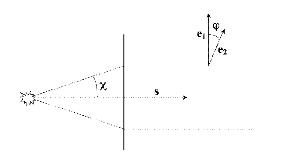
Figure 1:

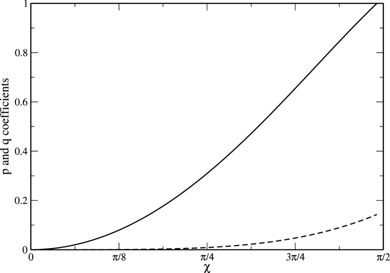
Figure 2:

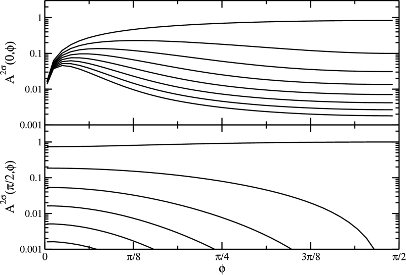
Figure 3:

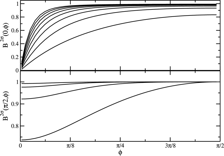
Figure 4:

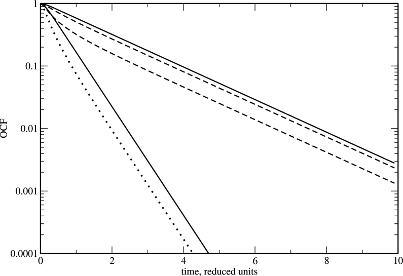
Figure 5:

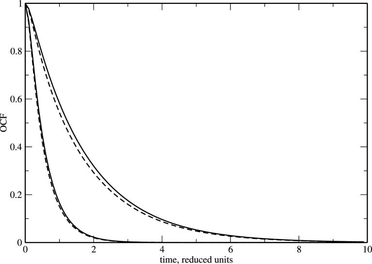
Figure 6:

References

- (1) R. G. Gordon, Adv. Magn. Reson. 3, 1 (1968).
- (2) R. E. D. McClung, Adv. Mol. Rel. Int. Proc. 10, 83 (1977).
- (3) A. I. Burshtein and S. I. Temkin. Spectroscopy of Molecular Rotations in Gases and Liquids (Cambridge University Press, Cambridge, 1994).
- (4) J. S. Baskin and A. H. Zewail, J. Phys. Chem. A 105, 3680 (2001).
- (5) S. Mukamel, Principles of Nonlinear Optical Spectroscopy (Oxford University Press, New York, 1995).
- (6) W. E. Moerner and M. Orrit, Science 283, 1670 (1999).
- (7) F. Kulzer and M. Orrit, Annu. Rev. Phys. Chem. 55, 585 (2004).
- (8) E. Barkai, Y. J. Jung and R. Stilbey, Annu. Rev. Phys. Chem. 55, 457 (2004).
- (9) I. S. Osadko, Uspekhi Fizicheskih Nauk 176, 23 (2006).
- (10) A. L. Buchachenko, Russian Chemical Reviews 75, 1 (2006).
- (11) T. Ha, T. A. Laurence, D. S. Chemla ans S. Weiss, J. Phys. Chem. B 103, 6839 (1999).
- (12) R. M. Dickson, D. J. Norris, and W. E. Moerner, Phys. Rev. Lett. 81, 5322 (1998).
- (13) B. Sick, B. Hecht, and L. Novotny, Phys. Rev. Lett. 85, 4482 (2000).
- (14) M. A. Lieb, J. M. Zavislan, and L. Novotny, J. Opt. Soc. Am. B 21, 1210 (2004).
- (15) M. Böhmer and J. Enderlein, J. Opt. Soc. Am. B 20, 554 (2003).
- (16) M. Vacha and M. Kotani, J. Chem. Phys. 118, 5279 (2003).
- (17) H. Uji-i, S. M. Melnikov, A. Deres, G. Bergamini, F. De Schryver, A. Herrmann, K. Müllen, J. Enderlein, and J. Hofkens, Polymer 47, 2511 (2006).
- (18) J. T. Fourkas, Optics Letters 26, 211 (2001).
- (19) J. Hohlbein and C. G. Hübner, Appl. Phys. Lett. 86, 121104 (2005).
- (20) L. A. Deschenes and D. A. Vanden Bout, J. Chem. Phys. 116, 5850 (2002).
- (21) E. Mei, J. Tang, J. M. Vanderkooi and R. M. Hochstrasser, JACS 125, 2730 (2003).
- (22) P. M. Wallace, D. R. B. Sluss, L. R. Dalton, B. H. Robinson, P. J. Reid, J. Phys. Chem. B 110, 75 (2006).
- (23) G. Hinze, G. Diezemann and Th. Basche, Phys. Rev. Lett. 93, 203001 (2004).
- (24) C.-Y. J. Wei, Y. H. Kim, R. K. Darst, P. J. Rossky, and D. A. Vanden Bout, Phys. Rev. Lett. 95, 173001 (2005).
- (25) M. F. Gelin and D.S. Kosov, J. Chem. Phys. 124, 144514 (2006).
- (26) M. P. Allen and D. J. Tildesley, Computer Simulation of Liquids (Clarendon Press, Oxford, 1991).
- (27) P. P. Feofilov, The Physical Basis of Polarized Emission. Consultants Bureau Enterprises, New York, 1961.
- (28) See Refs. wei99 ; boi04 for the effect of the optical system on the excitation cross-section.
- (29) A. Debarre, R. Jaffiol, C. Julien, D. Nutarelli, A. Richard, P. Tchenio, F. Chaput and J.-P. Boilot, Eur. Phys. J. D 28, 67 (2004).
- (30) G. S. Agrawal, Quantum Statistical Theories of Spontaneous Emission and Their Relation to Other Approaches (Springer Tracts in Modern Physics, Vol. 70, Springer-Verlag, Berlin, 1984).
- (31) If, prior to the collecting objective, the emitted photons pass through an interface, then Eq.(5) can be generalized as described, e.g., in Ref. end03
- (32) D. Axelrod, Biophys. J. 26, 557 (1979).
- (33) R. I. Cukier, J. Chem. Phys. 60, 734 (1974).
- (34) R. Tarroni and C. Zannoni, J. Chem. Phys. 95, 4550 (1991).
- (35) E. Berggren, R. Tarroni and C. Zannoni, J. Chem. Phys. 99, 6180 (1993).
- (36) D. A. Varshalovich, A. N. Moskalev and V. K. Hersonski. Quantum Theory of Angular Momentum (World Scientific, Singapore, 1989).
- (37) K. A. Valijev and E. N. Ivanov, Uspekhi Fizicheskih Nauk 109, 31 (1973).
- (38) R. I. Cukier and K. Lakatos-Lindenberg, J. Chem. Phys. 57, 3427 (1972).
- (39) S. R. Aragon R. Pecora, J. Chem. Phys. 64, 1791 (1976).
- (40) Other SM-relevant polarization CFs (see, e.g., Ref. ha04 ) can be calculated very similarly.
- (41) B. Stevens and T. Ha, J. Chem. Phys. 120, 3030 (2004).
- (42) W. A. Steele, J. Chem. Phys. 38, 2404 & 2411 (1963).
- (43) Within the fluorescence correlation spectroscopy, the analogue of Eq.(38) contains contributions from the OCFs the zeroth, second, and fourth rank. pec76
- (44) E. Mei, A. Sharonov, F. Gao, J. E. Ferris and R. M. Hochstrasser, J. Phys. Chem. A 108, 7339 (2004).
- (45) C. C. Wang and R. Pecora, J. Chem. Phys. 72, 5333 (1980).
- (46) A. Szabo, J. Chem. Phys. 81, 150 (1984).
- (47) D. Kivelson and T. Keyes, J. Chem. Phys. 57, 4599 (1972).
- (48) D. Kivelson and R. Miles, J. Chem. Phys. 88, 1925 (1988).
- (49) W. A. Steele, in Molecular liquids, NATO ASI Series C Vol. 135, edited by A. J. Barnes, W. J. Orville-Thomas and J. Yarwood (Reidel, Dordrecht, 1984), p. 111.
- (50) L. D. Favro, Phys. Rev. 119, 53 (1960).