Electron trapping by electric field reversal in glow discharges

Abstract

The phenomena of electric field reversal in glow discharges is discussed. Several models are described and the link between field reversal and the discharge structure is analyzed.

I Introduction

The phenomena of field reversal of the axial electric field in the negative glow of a dc discharge has been discussed since a long time in literature Raizer1 ; Engel1 . In a founding paper Druvestyn and Penning Druyvesteyn hypothesized its existence. Lawler et al.  Lawler1 assumed its existence when evaluating the current balance at the surface of a cold cathode discharge and estimated the position of the field reversal by linearly extrapolating the optical data of atomic transitions. The determination of the position where the field reversal occurs is of great importance since the fraction of ions returning to the cathode depends on its existence and location, and it is necessary for correctly determine the conditions for a self-sustained discharge.

Kolobov and Tsendin  Kolobov:92 have shown that the first field reversal is located near the end of the negative glow (NG), near the position (although located slightly to the cathode side) where ions density attains its greatest magnitude Gottscho:89 . If the discharge length has enough extension and the pressure decrease to lower values it appears a second field reversal on the boundary between the Faraday dark space and the positive column (PC)  Kolobov:92 ; Gottscho:89 .

Moreover, Kolobov and Tsendin explained how ions produced to the left of the first reversal location move to the cathode by ambipolar diffusion - helping to maintain the glow by secondary electron emission - and ions generated to the right of this location drift to the anode.

More recent work  Maric:02 ; Maric:03 presenting a comparison of experimental data and the predictions of a hybrid fluid-Monte Carlo model also supports the view that the point where the field is extrapolated to zero is practically coincident with the maximum of the emission (even when $j/p^{2}$ scaling is no longer valid). Those characteristics were experimentally observed by laser optogalvanic spectroscopy Gottscho:89 . For a detailed review see also Godyak .

Boeuf and Pitchford Boeuf with a simple fluid model gave an analytical expression of the field reversal location showing its dependency solely on the cathode sheath length, the gap length, and the ionization relaxation length. They obtained as well the fraction of ions arriving at the cathode and the magnitude of the plasma maximum density.

Technological application of gas discharges, particularly to plasma display panels, needs a better knowledge of the processes involved.

II Structure of a Glow Discharge

The phenomenology of DC glow discharges are well described, for example, by Roth Roth:95 , where the existence of the field reversal in the negative glow (NG) is already clearly shown. To be complete, we will recall now the most significant features with interest to our problem. In the regime of a normal glow discharge the voltage and the current density are both practically independent of the total current flowing in the discharge tube.

In a crude picture, energy is continuously transferred from a high voltage DC power source to the electrons originating from the cathode that accelerate absorbing energy from the field $eE$, ionizing, exciting and undergoing elastic collisions with heavy particles and other electrons. Electrons disappear basically by recombination and diffusion to the walls. Secondary electrons from the cathode provides an additional source of electrons and they have a prominent role in the discharge maintenance. The electric field decreases in the sheath, vary slowly in the plasma and increases again in the anode sheath, although not attaining such high value as in the cathode. All plasmas are separated from the walls (both conducting or non-conducting) by a sheath. The higher energies are attained by electrons which bombard far more frequently the walls than ions. The slower ions remaining behind build-up a positive plasma potential relative to the wall with a magnitude of the order of the electron kinetic temperature. In consequence ions are easily drawn off through the sheath by an external circuit as a current $I$ while electrons are repelled by the walls (and electrodes), only escaping the most energetic ones. As we proceed from the cathode to the anode we recognize several regions, first observed by Michael Faraday in the 1830’s, with interest to the present study (see also Refs. Roth:95 ; Laporte:39 ):

• Aston dark space - The electric field is very high and primary and secondary electrons outnumber ions. However, electrons have not still attained enough energy to excite neutrals and they have low density making this region to appear dark;

• cathode glow - electrons have already enough energy to excite neutrals and ions density increases;

• cathode (Crookes, Hittorf) dark space - Electrons are either too fast or too slow to excite the gas. The probability for fast electrons to excite are not negligible, however, and that’s why this regions is slightly brighter than the Aston dark space. In this region electrons have enough energy to ionize the gas and the ions production rate attains high magnitude, the dominant charge being positive. It is in this region that the primary electrons loose a great fraction of its energy in ionizing collisions and the generated secondary electrons appear with lower energy. Slow electrons are produced in this region. A moderate electric field dominates;

• cathode region (CR) - This is a transition region between the cathode dark space and the negative glow where most of the voltage drop (cathode fall) of $\phi_{c}$ at $x=d_{c}$. The axial length of the cathode region $d_{c}$ adjust its value in order to maintain a minimum value of the product $d_{c}p$, the Paschen minimum;

• negative glow (NG) - The electric field is here very low, but its luminosity results from the electrons that have been accelerated in the CR and ionize and excite neutrals in the NG (that’s why the luminosity is more intense on the CR side). As electrons lose their energy, recombinations processes are more probable, mainly in poliatomic electronegative gases to which electrons attach more easily. Electrons carry almost all the entire electric current in this region. Ionization in the glow can contribute significantly to the total ion current in the glow due to backscattered ions from the NG entering the cathode fall Dalvie:92 .

• Faraday dark space (FDS) - This region is located immediately to the right of the NG. Electrons energy is low and their density decreases due to recombination and radial diffusion. However, in gas discharge tubes with a radius much smaller than the discharge length, the electric field start to grow again and electrons gain energy giving birth to the positive column.

III Experimental observation of field reversal

The phenomenon of field reversal was experimentally observed by laser optogalvanic spectroscopy (LOG) firstly by Gottscho et al. Gottscho:89 . The LOG technique used was reported by Walkup et al. Walkup:83 and is based on a change of ion mobility on excitation by a dye laser. This means that an excited ion state with a larger (smaller) mobility will induce a transient current increase (decrease) on excitation. The sign of the LOG signal depends only on the sign of electric field reversal. Gottscho et al. Gottscho:89 at the same time recorded the $N_{2}^{+}(X^{2}\Sigma_{g}^{+})$ ions excited from its lowest and first excited vibrational levels (exciting the $B^{2}\Sigma_{u}^{+}-X^{2}\Sigma_{:}g^{+}$ (0,0) and (0,1) bands, respectively) using laser-induced fluorescence (LIF) along the plane parallel electrodes of their reactor. They noted that at low pressure the LOG signal changes sign near the position of the $N_{2}^{+}$ maximum while being located slightly to the cathode side. At higher pressure the field reversal occurs toward the anode side of the $N_{2}^{+}$ density maximum.

The LOG and LIF spatial profiles resulting from the excitation of the $B^{2}\Sigma_{u}^{+}-X^{2}\Sigma_{:}g^{+}$ (0,0) and (0,1) bands decrease first strongly to negative values due to the falloff in ion density, as it is registered by LIF. This is the pre-sheath Roth:95 , a quasi-neutral region between the plasma and the sheath characterized by small electric fields gradients (usually smaller than 1 V$/$cm). At a given position ions practically remain undetected by LIF, the LOG signal diminishes rapidly and this is a signature of the beginning of the cathode fall region.

IV Physical mechanism of the electric field reversals in glow discharges

Electric field reversals operate as a self-regulator mechanism of glow discharges. If electrons were in hydrodynamic equilibrium with the local electric field and were created in the cathode sheath followed by a fast diffusion to the walls and acceleration to the anode, then ions loss would occur through migration to the cathode and it will be no need for field reversal. This situation would be similar if the ionization main channels were ion and fast neutral impact ionization instead of electron impact ionization. However, electrons are not in equilibrium with the local electric field. This situation results from the complex structure embodied in the sheath, pre-sheath and plasma regions (see Ref. Roth:95 for details). The electric field decreases largely from the cathode surface within an adjacent region where the charged-particle density is low (e.g.,  Hartog:88 ). In this region electrons gain energy being strongly accelerated toward the bulk plasma attaining typically kinetic energies in the range $10\div 10^{3}$ eV. Thus, they are responsible of the excitation and ionization processes in the quasi-neutral region we call plasma. Clearly their energy is determined by the electron-energy spectrum and not by the local value of the electric field Shi .

Under typical gas discharge conditions it is possible to consider two groups of electrons: the group of slow and fast electrons. The majority of them belongs to the slow group of electrons; they are created in the quasi-neutral (bulk) plasma region through ionization and their kinetic energy does not exceed significantly the energy of the first excitation level $\epsilon_{1}$ Tsendin95 . The low electric field prevalent in the quasi-neutral region with a vast majority of slow electrons (with energies in the range $10^{-2}\div 10$ eV) is favorable to increase electrons loss while at the same time reducing ions loss. But as the total current density

$$\mathbf{j}=\mathbf{j}_{e}+\mathbf{j}_{i}=-en_{e}v_{e}+en_{i}v_{i}$$ (1)

must be constant along the discharge a mechanism of field reversal appears in order to enhance ions loss and reduce slow electrons loss. At the position where field reversal takes place the plasma potential presents a minimum value Gottscho:89 . This situation creates a kind of two contiguous reservoirs: to the left of the field reversal, ions generated by fast electrons flow to the cathode, where hitting the electrode surface induce secondary electrons emission at the cathode (and thus helping maintaining the glow); to the right of the field reversal, ions are accelerated toward the anode. As electrons diffuse more rapidly to the walls than ions, the walls along the positive column and near the anode sheath charge negatively, while along the cathode fall they charge positively (see, for example, Ref.  Laporte:39 ). This charge build-up deform the equipotentials surfaces that, instead to remain parallel to the electrodes, show the concave side facing the anode.

V Kolobov and Tsendin nonlocal kinetic model

Due to the complex self-consistent problem that is at stake, Kolobov and Tsendin endeavored to develop an analytical approach with a formidable complexity. Since the papers of Emeleus and co-workers  Emeleus:34 ; Emeleus:39 electrons have been divided in primary, secondary (or intermediate) and ultimate (or trapped) and so did Kolobov and Tsendin. The highly energetic electron created in the cathode sheath of a DC discharge have kinetic energies well above the first excitation potential $\varepsilon^{*}$. Ionization and excitation processes are created by them and they carry the electron current in the sheath and nearby plasma region. The plasma region is mainly populated by trapped electrons that do not contribute to the current. In the NG and FDS the current is mainly carried by (untrapped) intermediate electrons with energies below $\varepsilon^{*}$. The discharge gap is divided in two regions: the sheath and the (quasi-neutral) plasma region.

The fast electrons are described by a continuous-energy-loss model neglecting scattering

$$\frac{dw}{d\xi}=-N\mathcal{L}(w)-eE(x),$$ (2)

where $w$ is the electron kinetic energy, $N$ is the neutral particle density, $\mathcal{L}(w)$ is the energy-loss function, $\xi$ is the fast-electron path along its trajectory and $x$ is the spatial coordinate.

Neglecting scattering, then $\xi=x$ and the kinetic equation for fast electrons $F(v,x)$ is written under the form

$$v\frac{\partial F}{\partial x}-\frac{eE(x)}{m}\frac{\partial F}{\partial v}-\frac{\partial}{\partial v}\frac{N\mathcal{L}(w)}{m}F=J(x,v).$$ (3)

Here, $J(x,v)$ is a source term and it was assumed $\mathcal{L}(w)=\mathcal{L}_{0}=const$. Its integration is performed at constant energy

$$\varepsilon=w+N\mathcal{L}_{0}x-e\phi(x)=w-e\tilde{\phi}(x),$$ (4)

where $\phi(x)$ is the electrostatic potential obtained for linear-electric field profile in the sheath. The fast electrons start riding on an effective potential, $e\tilde{\phi}(x)$, that attains a minimum in a point where the total force is zero, $eE(\tilde{d})=N\mathcal{L}_{0}$ (see Fig.2). For example, for He, $\mathcal{L}_{0}=1.5\times 10^{-15}$ eV cm². Solving Eq. 3 it is obtained the fast-electron current

$$j_{f}(x)=e\int_{0}^{\infty}vdvF(v,x)=$$

$$j_{f}(x)=\left\{\begin{array}[]{cc}e\Gamma_{e}\exp(\alpha x),&0<x<\tilde{d}\\ j_{f}(x_{0}(\varepsilon=e\mathcal{\phi}(x))),&\tilde{d}<x<x_{1}(e\tilde{\phi}_{c}),\end{array}\right.$$ (5)

where $\alpha=N\mathcal{L}_{0}/\varepsilon_{0}$, with $\varepsilon_{0}$ denoting the constant energy loss per ion-electron pair and $\Gamma_{e}$ is the electron flux from the cathode. Notice that for $x<\tilde{d}$ the total electron current $j_{e}$ is equal to the fast-electron current $j_{f}$ and that, in particular, we have

$$\frac{dj_{e}}{dx}=\alpha j_{f}=I(x).$$ (6)

Here, $I(x)$ is the ionization density. Eqs. 5 and  6 constitute a generalization of the Townsend approach with a constant ionization coefficient $\alpha=const.$

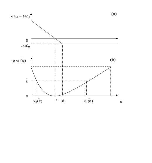
Figure 1: a) Total force acting on an electron under constant energy-loss; b) effective potential energy of electrons, $e\tilde{\phi}(x)$)

At $x>x_{1}(e\tilde{\phi}_{c})$ there is no ionization source since the fast electrons do not reach this region; this region limits the boundary between the FDS and NG (see Sec. 2 for its characterization) and the length of the NG is given qualitatively by $R=e\phi_{c}/\alpha\varepsilon_{0}$.

For slow electrons with $w<\varepsilon^{*}$ the continuous-energy-loss is no longer valid and it is essential to take into account the essential discrete character of the energy loss, where elastic and electron-electron collisions are the only energy-relaxation mechanisms. If $L$ is bigger than the electron mean free path $\lambda$, then the electron energy distribution function (EDF) is isotropic and the two-term expansion in spherical harmonics holds. Hence, taking into account the following contributions: i) degradation of fast electrons injected into the plasma from the cathode sheath; ii) slow electrons generation by fast electrons; iii) slow electrons superelastic collisions with molecular low vibrational levels or others, with kinetic energy slightly exceeding $\varepsilon^{*}$, the kinetic equation for the isotropic part of the EDF gives for the trapped electrons a Maxwell-Boltzmann distribution of the type:

$$f_{0}^{(t)}=\left(\frac{m}{2\pi T_{e}}\right)^{2/3}n_{m}[\exp(-\varepsilon/T_{e})-\exp(-e\phi_{a}/T_{e})],$$ (7)

where $\phi_{a}$ denotes the anode potential and $n_{m}$ is the maximum trapped electron density at the point of field reversal $E(x)=0$. The electron temperature is obtained by solving the integral energy balance for trapped electrons, but in a first approach we have $e\phi_{a}\sim T_{e}$. For example, by laser diagnostics experiments Hartog:88 the slow electron temperature and density are $T_{e}=0.2$ eV and $n_{m}=1.2\times 10^{12}$ cm³in He at $p=3.5$ Torr, with an electrode gap $L=0.62$ cm and $j=0.846$ mA$/$ cm². The trapped electrons give the main contribution to the plasma density

$$n_{s}(x)=\frac{4\pi}{m}\int_{-e\phi(x)}^{\varepsilon^{*}}v(\varepsilon,x)f_{0}(\varepsilon,x)d\varepsilon,$$ (8)

while giving zero contribution to the slow-electrons current density:

$$j_{s}(x)=\frac{4\pi e}{3m}\int_{-e\phi(x)}^{\varepsilon^{*}}v(\varepsilon,x)D(\varepsilon,x)\frac{\partial f_{0}}{\partial x}d\varepsilon.$$ (9)

The $j_{s}$ is the the total electron current in the FDS represented by the transport of the intermediate untrapped electrons. In the low-pressure limit the trapped electrons are expected to be isothermal and to be governed by the ambipolar diffusion equation:

$$\frac{d}{dx}\left(D_{a}\frac{dn}{dx}\right)+I(x)-\frac{n}{\tau}=0.$$ (10)

Here, $\tau=\Lambda^{2}/D_{a}$. Eq. 10 can be solved using the Green’s function approach with appropriate boundary conditions. It gives the minimum $x_{m}$:

$$\int_{d}^{L}xI(x)dx=(L+d)\int_{x_{m}}^{L}I(x)dx.$$ (11)

The position of $x_{m}$ determines the ratio of ions returning to the cathode. If the FDS length $(L-R)$ exceeds $(R-d)$ then $x_{m}\to R$ and the majority of ions generated in the plasma return to the cathode; if, on the contrary, $R-d>L-R$ this means that fast electrons penetrate deep in the plasma, the majority of them attaining the anode. In their calculation the position of maximum ions density coincides with the field reversal location. Unfortunately, Kolobov and Tsendin do not give explicit expression for $x_{m}$, introducing an error in Eq. 11 (see remark in Ref. Kudryavtsev:05 ).

To resume the previous work by Kolobov and Tsendin Kolobov:92 , the study of nonlocal phenomena in electron kinetics of collisional gas discharge plasma have shown that in the presence of field reversals the bulk electrons in the cathode plasma are clearly separated in two groups of slow electrons: trapped and free electrons. Trapped electrons give no contribution to the current but represent the majority of the electron population. The first field reversal it was shown qualitatively to be located near the end of the negative glow (NG) where the plasma density attains the greatest magnitude. If the discharge length is long enough, it appears a second field reversal on the boundary between the Faraday dark space and the positive column. Also, it was shown that ions produced to the left of this first reversal location move to the cathode by ambipolar diffusion and ions generated to the right of this location drift to the anode. For a review see also Godyak .

VI Boeuf and Pitchford fluid model

Boeuf et al Boeuf with a simple fluid model gave an analytical expression of the field reversal location which showed to depend solely on the cathode sheath length, the gap length, and the ionization relaxation length. They obtained as well a simple analytical expression giving the fraction of ions returning to the cathode and the magnitude of the plasma maximum density.

Their model assumes a spatial profile of the ionization rate $S_{T}(x)=N_{e}(x)\nu_{i}(x)$ in a plasma being formed in a parallel plate geometry. Monte Carlo calculations show that the ionization rate is linear in the sheath and decreases exponentially in the NG Peres:92 and so they assumed

$$S_{T}(x)=\left\{\begin{array}[]{ll}0&\mbox{,for $x<d_{c}$}\\ s\exp(-\frac{x-d_{c}}{\lambda_{\varepsilon}})&\mbox{,for $x\geq d_{c}$}.\end{array}\right.$$ (12)

Here, $\lambda_{\varepsilon}$ is the energy relaxation length of the high electrons energy entering the NG accelerated in the sheath while $s$ is a function of the voltage $\phi_{c}$, gas mixture and is proportional to the flux of secondary electrons leaving the cathode $\Gamma_{e0}$ (here, $e$ (electrons) and $i$ (ions) denotes the specie). They assume that slow electrons can be described by a continuity equation and a momentum transport equation in the drift-diffusion approximation (and thus considering drift energy negligible with respect to thermal energy):

$$\frac{d\Gamma_{e0}}{dx}=S_{T}(x),$$ (13)

with

$$\Gamma_{e0}=\mp n_{e,i}\mu_{e,i}E-D_{e,i}\frac{dn_{e,i}}{dx},$$ (14)

where $\mu_{e,i}$ and $D_{e,i}$ denote the electron and ion mobility and diffusion coefficients respectively. Quasi-neutrality ($n=n_{e}\sim n_{i}$) is assumed in the NG region. The total current density is given by the expression

$$J_{T}=e(-\phi_{e}+\phi_{i}).$$ (15)

From this equation, together with Eq. 14, it is obtained the electric field

$$E(x)=\frac{J_{T}}{en_{e}(\mu_{e}+\mu_{i})}-\frac{D_{e}-D_{p}}{\mu_{e}+\mu_{i}}\frac{1}{n}\frac{dn}{dx},$$ (16)

where the electron and ion fluxes are now given by

$$\phi_{e}(x)=-\frac{J_{T}\mu_{e}}{e(\mu_{e}+\mu_{i})}-D_{a}\frac{dn}{dx},$$ (17)

and

$$\phi_{i}(x)=-\frac{J_{T}\mu_{i}}{e(\mu_{e}+\mu_{i})}-D_{a}\frac{dn}{dx}.$$ (18)

Here, $D_{a}$ is the ambipolar diffusion coefficient given by

$$D_{a}=\frac{\mu_{e}D_{i}+\mu_{i}D_{e}}{\mu_{e}+\mu_{i}}.$$ (19)

Integrating Eq. 13 and taking into account the ionization source terms in Eq. 12 it is obtained

$$\Gamma_{e}(x)=\left\{\begin{array}[]{ll}\Gamma_{e0}&\mbox{,for $x<d_{c}$}\\ \Gamma_{e0}+s\lambda_{\varepsilon}[1-a(x)]&\mbox{,for $x\geq d_{c}$},\end{array}\right.$$ (20)

using the simplifying notation $a(x)=\exp[-(x-d_{c})/\lambda_{\varepsilon}]$. At some position $x_{m}$ it can possibly occur a field reversal, located at a boundary that split the ion flux at the right side toward the anode and keeping electrons confined in the plasma region while at the left side directing the ion flux toward the cathode. Hence, a condition can be stated of a total current at some yet unspecified position $x_{0}$ (in this Sec. we use this notation for the field reversal location) being equal to the electron current:

$$J_{T}=-e\Gamma_{e}(x_{0})=-e\{\Gamma_{e0}+s\lambda_{\varepsilon}[1-a(x_{0})]\}.$$ (21)

From Eq. 17 and Eq. 20, using Eq. 21, it is obtained the following first order differential equation for $x\geq d_{c}$:

$$1+\frac{s\lambda}{\phi_{e0}}[1-a(x)]=\frac{\mu_{e}}{(\mu_{e}+\mu_{i})}\left(1+\frac{s\lambda}{\phi_{e0}}[1-a(x_{0})]-\frac{D_{a}}{\phi_{e0}}\frac{dn}{dx}\right).$$ (22)

Integrating Eq. 22 between $d_{c}$ and $L$ with appropriate boundary conditions, $n(d_{c})=n(d)=0$, under the approximation $\mu_{i}\ll\mu_{e}$, it is obtained

$$a(x_{0})=\frac{\lambda}{d-d_{c}}[1-a(d)].$$ (23)

Introducing the dimensionless parameter $\Lambda=\lambda/(d-d_{c})$, representing the ratio of the relaxation length to the distance between the anode and the CR boundary, Eq. 23 can be written under the form

$$\frac{x_{0}-d_{c}}{L-d_{c}}=-\Lambda\ln[\Lambda(1-\exp(-1/\Lambda)].$$ (24)

The above equation shows that, by one side, the position of the field reversal $x_{0}$ depends on the cathode sheath length $d_{c}$, the gap length $L$ and on the electron energy relaxation length $\lambda_{\varepsilon}$. By other side, $d_{c}$ and $\lambda_{\varepsilon}$ depend on the cathode sheath voltage and gas mixture. As can be seen in Fig. 2, when $\lambda_{\varepsilon}\ll L$ (low values of $\Lambda$) the position of the field reversal is near the plasma-sheath boundary; when $\lambda_{\varepsilon}\gg L$ (large values of $\Lambda$) the position of the field reversal is displaced to the mid-distance between the gap length and the plasma-sheath boundary. This last case occurs for an obstructed discharge, i.e, when the gap length is less than the Paschen minimum $d_{c}$ at the Paschen minimum.

Figure 2: Position of the field reversal, $\frac{x_{0}-d_{c}}{L-d_{c}}$, as a function of the adimensional parameter $\Lambda$.

The fractions of ions to the cathode can be determined using the relationship

$$\eta=\frac{\int_{0}^{x_{0}}S_{T}(x)dx}{\int_{0}^{L}S_{T}(x)dx}=\frac{\phi_{e}(x_{0})-\phi_{e0}}{\phi_{e}(L)-\phi_{e0}}.$$ (25)

We can give an explicit form to this ratio using Eq. 20 and Eq. 24:

$$\eta=\frac{1}{1-\exp(-\/\Lambda)}-\Lambda.$$ (26)

This fraction depends only on $\Lambda$ and, as Fig. 3 illustrate, its values are between $0.5$ and $1$.

Figure 3: Fraction of ions returning to the cathode as a function of the adimensional parameter $\Lambda$.

Fig. 3 shows that when the electron energy relaxation length $\lambda_{\varepsilon}$ is smaller than the gap length, $\eta\to 1$, the major fraction of ions return to the cathode. This is true if radial diffusion to the walls or recombination is not accounted for. In the condition of an obstructed discharge $\lambda_{\varepsilon}\gg L$, then $\eta\to 0.5$. Taking into account radial diffusion and recombination will lower the fraction of ions returning to the cathode.

Integrating Eq. 22 between $x=d_{c}$ and a given $x$, considering appropriate boundary conditions, $n(d_{c})=n(L)=0$, assuming $\mu_{i}\ll\mu_{e}$ and using Eq. 23 it is obtained readily

$$n(x)=\frac{s\lambda_{\varepsilon}^{2}}{D_{a}}(1-\exp(-1/\Lambda))\left(\frac{1-\exp(-\chi/\Lambda)}{1-\exp(-1/\Lambda)}-\chi\right),$$ (27)

with $\chi=\frac{x-d_{c}}{L-d_{c}}$. The plasma density attains a maximum at the position where occurs the field reversal $x_{0}$. This is inconsistent with Eq. 16, however, since here it was neglected the ions mobility in regard of the electrons mobility. In fact, the maximum of the plasma density is located near the position of the field reversal, but its maximum should be located to the cathode side of the field reversal. Maric et al. Maric:02 ; Maric:03 showed a perfect agreement of the analytical formula given in Eq. 24 with an hybrid Monte Carlo-fluid model. Kudryavtsev and Toinova Kudryavtsev:05 determined the position of the field reversal from the position of maximum ion density in the plasma. Their approach is quite simple giving simple analytical formulas in a short (without positive column) DC glow discharge making use of the ionization rate coefficients for fast electrons in the field.

VII A Dielectric-like model of field reversal

In this section we introduce a quite simple dielectric-like model of a plasma-sheath system Pinheiro:04 . This approach have been addressed by other authors Taillet69 ; Harmon76 to explain how the electrical field inversion occurs at the interface between the plasma sheath and the beginning of the negative glow. The aim of this Letter is to obtain more information about the fundamental properties related to field inversion phenomena in the frame of a dielectric model. It is obtained a simple analytical dependence of the axial location where field reversal occurs in terms of macroscopic parameters. In addition, it is obtained the magnitude of the minimum electric field inside the through, the trapped well length, and the trapping time of the slow electrons into the well. We emphasize in particular the description of the dielectric behavior and do not contemplate plasma chemistry and plasma-surface interactions.

The analytical results hereby obtained could be useful for hybrid fluid-particle models (e.g., Fiala et al. Boeuf94 ), since simple criteria can be applied to accurately remove electrons from the simulations.

On the ground of the stress-energy tensor considerations it is shown the inherent instability of the field inversion sheath. The slow electrons distribution function is obtained assuming the Fermi Fermi mechanism responsible for their acceleration from the trapping well.

Lets consider a plasma formed between two parallel-plate electrodes due to an applied dc electric field. We assume a planar geometry, but extension to cylindrical geometry is straightforward. The applied voltage is $V_{a}$ and we assume the cathode fall length is $l$ and the negative glow + eventually the positive column extends over the length $l_{0}$, such that the total length is $L=l+l_{0}$. We have

$$-V_{a}=lE_{s}+l_{0}E_{p},$$ (28)

where $E_{s}$ and $E_{p}$ are, resp., the electric fields in the sheath and NG (possibly including the positive column).

At the end of the cathode sheath it must be verified the following boundary condition by the displacement field $\mathbf{D}$

$$\mathbf{n}.(\mathbf{D}_{p}-\mathbf{D}_{s})=\sigma.$$ (29)

Here, $\sigma$ is the surface charge density accumulated at the boundary surface and $\mathbf{n}$ is the normal to the surface. In more explicit form,

$$\varepsilon_{p}E_{p}-\varepsilon_{s}E_{s}=\sigma.$$ (30)

Here, $\varepsilon_{s}$ and $\varepsilon_{p}$ are, resp., the electrical permittivity of the sheath and the positive column. We have to solve the following algebraic system of equations

$$\begin{array}[]{cc}l_{0}E_{p}+lE_{s}&=-V_{a},\\ \varepsilon_{p}E_{p}-\varepsilon_{s}E_{s}&=\sigma.\\ \end{array}$$ (31)

They give the electric field strength in each region

$$\begin{array}[]{cc}E_{s}=&-\frac{V_{a}}{L}\left(1-\alpha+\frac{l_{o}\sigma}{V_{a}\varepsilon_{s}}\right)\frac{1}{1-\frac{l\alpha}{L}},\\ E_{p}=&-\frac{V_{a}}{L}\left(1-\frac{l\sigma}{V_{a}\varepsilon_{s}}\right)\frac{1}{1-\frac{l\alpha}{L}}.\\ \end{array}$$ (32)

Here, we define $\alpha=1-\frac{\varepsilon_{p}}{\varepsilon_{s}}=\frac{\omega_{p}^{2}}{\nu_{en}^{2}}$. Recall that in DC case, $\varepsilon_{p}=1-\frac{\omega_{p}^{2}}{\nu_{en}^{2}}$, and $\varepsilon_{s}=\varepsilon_{0}$, with $\omega_{p}$ denoting the plasma frequency and $\nu_{en}$ the electron-neutral collision frequency. In fact, our assumption $\varepsilon_{s}=\varepsilon_{0}$ is plainly justified, since experiments have shown the occurrence of a significant gas heating and a corresponding gas density reduction in the cathode fall region, mainly due to symmetric charge exchanges processes which lead to an efficient conversion of electrical energy to heavy-particle kinetic energy and thus to heating Hartog:88 .

Two extreme cases can be considered: i) $\omega_{p}>\nu_{en}$, implying $\varepsilon_{p}<0$, meaning that $\tau_{coll}>\tau_{plasma}$, i.e, non-collisional regime prevails; ii) $\omega_{p}<\nu_{en}$, $\varepsilon_{p}>0$, and then $\tau_{coll}>\tau_{plasma}$, i.e, collisional regime dominates.

From the above Eqs. 32 we estimate the field inversion should occurs for the condition $1-\frac{l_{o}\alpha}{L}=0$, which give the position on the axis where field inversion occurs:

$$\frac{l_{o}}{L}=\frac{\nu_{en}^{2}}{\omega_{p}^{2}}.$$ (33)

From Eq. 33 we can resume a criteria for field reversal: it only occurs in the non-collisional regime; by the contrary, in the collisional regime and to the extent of validity of this simple model, no field reversal will occur, since the slow electrons scattering time inside the well is higher than the the well lifetime, and collisions (in particular, coulombian collisions) and trapping become competitive processes. A similar condition was obtained in Nishikawa69 when studying the effect of electron trapping in ion-wave instability. Likewise, a self-consistent analytic model Kolobov:92 have shown that at at sufficiently high pressure, field reversal is absent.

Due to the accumulation of slow electrons after a distance $\xi_{c}=L-l_{0}$, real charges accumulated on a surface separating the cathode fall region from the negative glow. Naturally, it appears polarization charges on each side of this surface and a double layer is created with a surface charge $-\sigma_{1}^{\prime}<0$ on the cathode side and $\sigma_{2}^{\prime}$ on the anode side. But, $\sigma^{\prime}=(\mathbf{P}\cdot\mathbf{n})$, $\mathbf{P}=\mathbf{\mathbf{\varepsilon}_{0}}\chi_{e}\mathbf{E}$ with $\varepsilon=\varepsilon_{0}(1+\chi_{e})$, $\chi_{e}$ denoting the dimensionless quantity called electric susceptibility. As the electric displacement is the same everywhere, we have $\mathbf{D}_{0}=\mathbf{D}_{1}=\mathbf{D}_{2}$. Thus, the residual (true) surface charge in between is given by

$$\sigma=-\sigma_{1}^{\prime}+\sigma_{2}^{\prime}.$$ (34)

After a straightforward but lengthy algebraic operation we obtain

$$\sigma=\varepsilon_{p}V_{a}\frac{B}{A},$$ (35)

where

$$A=L\left(-1+\frac{\varepsilon_{0}-\varepsilon_{s}}{\varepsilon_{p}}\right)+l\left(-\frac{\varepsilon_{p}}{\varepsilon_{s}}+\frac{\varepsilon_{s}}{\varepsilon_{p}}\right),$$ (36)

and

$$B=\frac{\varepsilon_{0}(\varepsilon_{s}-\varepsilon_{p})}{\varepsilon_{s}\varepsilon_{p}}.$$ (37)

We can verify that $\sigma$ must be equal to

$$\sigma=\alpha\frac{V_{a}\varepsilon_{0}}{2l_{0}}.$$ (38)

Considering that $\sigma=\varepsilon_{0}\chi_{e}E$, we determine the minimum value of the electric field at the reversal point:

$$E_{m}=\frac{\omega_{p}^{2}}{\nu_{en}^{2}}\frac{V_{a}}{2l_{0}\chi_{e}}.$$ (39)

Here, $\chi_{e}=\varepsilon_{rw}-1$, with $\varepsilon_{rw}$ designating the relative permittivity of the plasma trapped in the well. From the above equation we can obtain a more practical expression for the electrical field at its minimum strength

$$E_{m}=-\frac{n_{ep}}{n_{ew}}\frac{\nu_{enw}^{2}}{\nu_{en}^{2}}\frac{V_{a}}{el_{0}}\approx-\frac{n_{ep}}{n_{ew}}\frac{T_{ew}}{T_{ep}}\frac{V_{a}}{2l_{0}}.$$ (40)

The magnitude of the minimum electric field depends on the length of the negative glow $l_{0}$. This also means that without NG there is no place for field reversal, and also the bigger the length the minor the electric field. The length of the negative glow can be estimated by the free path length $l_{0}$ of the fastest electrons possessing an energy equal to the cathode potential fall value $eV_{a}$:

$$l_{0}=\int_{0}^{eV_{a}}\frac{dw}{(NF(w))}.$$ (41)

Here, $w$ is the electrons kinetic energy and $NF(w)$ is the stopping power. For example, for He, it is estimated $pl_{0}=0.02eV_{a}$  Kolobov:92 (in cm.Torr units, with $V_{a}$ in Volt). We denote by $n_{ew}$ the density of trapped electrons and by $T_{ew}$ their respective temperature. Altogether, $n_{ep}$ and $T_{ep}$ are, resp., the electron density and electron temperature in the negative glow region.

By other side, we can estimate the true surface charge density accumulated on the interface of the two regions by the expression

$$\sigma=\frac{Q}{A}=-\frac{n_{ep}eA\Delta\xi}{A}.$$ (42)

Here, $Q$ is the total charge over the cross sectional area where the current flows and $\Delta\xi$ is the width of the potential well.

VII.1 Instability and width of the potential well

From Eqs. 38 and  42 it is easily obtained the trapping well width

$$\Delta\xi=-\frac{eV_{a}}{2ml_{0}\nu_{enw}^{2}}.$$ (43)

It is expected that the potential trough should have a characteristic width of the order in between the electron Debye length ($\lambda_{De}=\sqrt{\frac{\varepsilon_{0}kT_{e}}{n_{e}e^{2}}}$) and the mean scattering length. Using Eq. 43, in a He plasma and assuming $V_{a}=1$ kV, $l_{0}=1$ m and $\nu_{en}=1.85\times 10^{9}$ s^-1 (with $T_{e}=0.03$ eV) at 1 Torr ($n=3.22\times 10^{16}$ cm^-3) we estimate $\Delta\xi\approx 2.6\times 10^{-3}$ cm, while the Debye length is $\lambda_{De}=2.4\times 10^{-3}$ cm. So, our Eq. 43 gives a good order of magnitude for the potential width, which is expected to be in fact of the same order of magnitude than the Debye length.

Table I present the set of parameters used to obtain our estimations. We give in Table II the estimate of the minimum electric field attained inside the well. The first field reversal at $\xi_{c}\approx l_{NG}$ corresponds to the maximum density $n_{ew}\gg n_{ep}$ Boeuf ; Tsendin2001 . So, the assumed values for the ratio of electron temperatures and densities of the trapped electrons and electrons on the NG are typical estimates.

Table 1: Data used for $E/p=100$ V$/$cm$/$Torr. Cross sections and electron temperatures are taken from Siglo Data base, CPAT and Kinema Software, http://www.Siglo-Kinema.com

Gas	$T_{e}$ (eV)	$\sigma$ ($10^{-16}$ cm2)
Ar	8	4.0
He	35	2.0
O2	6	4.5
N2	4	9.0
H2	8	6.0

It can be shown that there is no finite configuration of fields and plasma that can be in equilibrium without some external stress Longmire . Consequently, this trough is dim to be unstable and burst electrons periodically (or in a chaotic process), releasing the trapped electrons to the main plasma. This phenomena produces local perturbation in the ionization rate and the electric field giving rise to ionization waves (striations). In the next section, we will calculate the time of trapping with a simple Brownian model.

Table 2: Minimum electric field at reversal point and well width. Conditions: He gas, $p=1$ Torr, $l_{0}=20$ cm, $V_{a}=1$ kV, $\frac{T_{ew}}{T_{ep}}=0.1$, $\frac{n_{ew}}{n_{ep}}=10$.

$E_{m}$ (V.cm-1)	$\Delta\xi$ (cm)
$\lesssim-2.5$	$2.6\times 10^{-3}$

From Eq. 33 we calculate the cathode fall length for some gases. For this purpose we took He and H₂ data as reference for atomic and molecular gases, resp. The orders of magnitude are the same, with the exception of Ar. Due to Ramsauer effect direct comparison is difficult.

In Table III it is shown a comparison of the experimental cathode fall distances to the theoretical prediction, as given by Eq. 43. Taking into account the limitations of this model these estimates are well consistent with experimental data Brown59 .

Table 3: Comparison between theoretical and experimental cathode fall distance at p=1 Torr, $E/p$=100 V$/$cm$/$Torr. Experimental data are collected from Ref. Brown59 .

Gas	$\xi_{c}^{teo}$ (cm)	$\xi_{c}^{exp}$ (cm)
Ar	7.40	0.29 (Al)
He	1.32	1.32 (Al)
$H_{2}$	0.80	0.80 (Cu)
$N_{2}$	0.45	0.31 (Al)
$Ne$	0.80	0.64 (Al)
$O_{2}$	0.30	0.24 (Al)

VII.2 Lifetime of a slow electron in the potential well

The trapped electrons most probably diffuse inside the well with a characteristic time much shorter than the lifetime of the through. Trapping can be avoided by Coulomb collisions Nishikawa69 or by the ion-wave instability, both probably one outcome of the stress energy unbalance as previously mentioned. We consider a simple Brownian motion model for the slow electrons to obtain the scattering time $\tau$, and the lifetime T of the well. A Fermi-like model will allow us to obtain the slow electron energy distribution function.

Considering the slow electron jiggling within the well, the estimated scattering time is

$$\tau=\frac{(\Delta\xi)^{2}}{\mathcal{D}_{e}}.$$ (44)

Here, $\mathcal{D}_{e}$ is the electron diffusion coefficient at thermal velocities.

Table 4: Scattering time and trapping time in the well. The parameters are: $E/N=100$ Td, $T_{g}=300$ K, $V_{a}=1$ kV and $l_{0}=0.1$ m.

Gas	$\mathcal{D}_{e}$ (cm2.s-1)	$\nu_{enw}(s^{-1})$	$\Delta\xi(cm)$	$\tau$ (s)	T (s)
Ar	$2.52\times 10^{6}$	$8.10\times 10^{9}$	$1.34\times 10^{-3}$	$7.10\times 10^{-13}$	$3.97\times 10^{-5}$
He	$5.99\times 10^{6}$	$2.39\times 10^{9}$	$1.54\times 10^{-2}$	$3.95\times 10^{-11}$	$1.70\times 10^{-5}$
N2	$6.11\times 10^{5}$	$6.15\times 10^{9}$	$2.32\times 10^{-3}$	$8.81\times 10^{-12}$	$1.64\times 10^{-4}$
CO2	$1.70\times 10^{6}$	$3.60\times 10^{9}$	$6.78\times 10^{-3}$	$2.70\times 10^{-11}$	$5.90\times 10^{-5}$

The fluctuations arising in the plasma are due to the breaking of the well and we can estimate the amplitude of the fluctuating field by means of Eq. 40. We obtain

$$\delta E_{m}=\frac{n_{ep}}{n_{ew}}\frac{\nu_{enw}^{2}}{\nu_{en}^{2}}\frac{V_{a}}{el_{0}^{2}}\Delta\xi.$$ (45)

Then, we have

$$\mathcal{E}_{c}=\frac{\delta E_{m}}{E_{m}}=\frac{\Delta\xi}{l_{0}}.$$ (46)

In Table IV we summarize scattering and trapping times for a few gases.

VII.3 Power-law slow electrons distribution function

As slow electrons are trapped by the electric field inversion, some process must be at work to pull them out from the well. We suggest that fluctuations of the electric field in the plasma (with order of magnitude of $\mathcal{E}_{c}$)act over electrons giving energy to the slow ones, which collide with those irregularities as with heavy particles. From this mechanism it results a gain of energy as well a loss. This model was first advanced by E. Fermi Fermi when developing a theory of the origin of cosmic radiation. We shall focus here on the rate at which energy is acquired.

The average energy gain per collision by the trapped electrons (in order of magnitude) is given by

$$\Delta w=\overline{U}w(t),$$ (47)

with $\overline{U}\cong\mathcal{E}_{c}^{2}$ and where $w$ is their kinetic energy. After $N$ collisions the electrons energy will be

$$w(t)=\varepsilon_{t}\exp\left(\frac{\overline{U}t}{\tau}\right),$$ (48)

with $\varepsilon_{t}$ being their thermal energy, typical of slow electrons.

Figure 4: Slow electrons distribution function vs. energy, for the same conditions as presented in Table 4. Solid curve: Ar, broken curve: N₂.

The time between scattering collisions is $\tau$. Assuming a Poisson distribution $P(t)$ for electrons escaping from the trapping, then we state

$$P(t)=\exp(-t/\tau)dt/T.$$ (49)

The probability distribution of the energy gained is a function of one random variable (the energy), such as

$$f_{w}(w)dw=P\{w<\bar{w}<w+dw\}.$$ (50)

This density $f_{w}(w)$ can be determined in terms of the density P(t). Denoting by $t_{1}=T$ the real root of the equation $w=w(t_{1}=T)$, then it can be readily shown that slow electrons obey in fact to the following power-law distribution function

$$f_{w}(w)dw=\frac{\tau}{\bar{U}T}\varepsilon_{t}^{\frac{\tau}{\bar{U}T}}\frac{dw}{w^{1+\tau/\bar{U}T}}.$$ (51)

Like many man made and naturally occurring phenomena (e.g., earthquakes magnitude, distribution of income), it is expected the trapped electron distribution function to be a power-law (see Eq. 51), hence $1+\frac{\tau}{\mathcal{E}_{c}^{2}T}=n$, with $n=2\div 4$ as a reasonable guess. Hence, we estimate the trapping time to be

$$T\approx\frac{\tau}{\mathcal{E}_{c}^{2}n}.$$ (52)

Fig.1 shows the slow electrons distribution function pumped out from the well for two cases: Ar (solid curve), and N₂ (broken curve). It was chosen a power exponent $n=2$. Those distributions show that the higher confining time is associated with less slow electrons present in the well. When the width of the well increases (from solid to broken curve) the scattering time become longer, and as well the confining time, due to a decrease of the relative number of slow electrons per given energy. This mechanism of pumping out of slow (trapped) electrons from the well can possibly explains the generation of electrostatic plasma instabilities.

Note that the trapping time is, in fact, proportional to the length of the NG and inversely proportional to the electrons diffusion coefficient at thermal energies:

$$T\approx\frac{l_{0}^{2}}{\mathcal{D}_{e}}.$$ (53)

The survival frequency of trapped electrons is $\nu_{t}=1/T$. As the electrons diffusion coefficient are typically higher in atomic gases, it is natural to expect plasma instabilities and waves with higher frequencies in atomic gases. This result is in agreement with a kinetic analysis of instabilities in microwave discharges Tatarova1 . In addition, the length of the NG will influence the magnitude of the frequencies registered by the instabilities, since wavelengths have more or less space to build-up. Table 4 summarizes the previous results for some atomic and molecular gases. The transport parameters used therefor where calculated by solving the electron Boltzmann equation, under the two-term approximation, in a steady-state Townsend discharge Pinheiro .

VIII Conclusion

This paper reviews, and extends when necessary, the physics of the electric field reversals in a glow discharge. We listed and studied how the structure of a glow discharge is related to the electrons and ions kinetics, described related experimental results, and have shown how the field reversals help to maintain the discharge. To this end different methods to describe the different groups of electrons generated in a glow discharge have been presented: the nonlocal approach of Kolobov and Tsendin Kolobov:92 ; the simple analytic fluid model by Boeuf and Pitchford Boeuf ; the theoretical analysis developed by Kudryavtsev and Toinova Kudryavtsev:05 , and the dielectric-like model Pinheiro:04 .

References

- (1) Yu. P. Raizer, Physics of Gas Discharge (Nauka, Moscow, 1992)
- (2) A. von Engel, Ionized Gases (Clarendon Press, Oxford, 1965)
- (3) M. J. Druyvesteyn and F. M. Penning, Rev Mod. Phys. 12 (2) 87 (1940)
- (4) D. A. Doughty, E. A. Den Hartog, and J. E. Lawler, Phys. Rev. Lett. 58 (25) 2668 (1987)
- (5) V. I. Kolobov and L. D. Tsendin, Phys. Rev. A 46(12), 7837 (1992)
- (6) Richard A. Gottscho, Annette Mitchell, Geoffrey R. Scheller, Yin-Yee Chan, David B. Graves, Phys. Rev. A, 40(1), 6407 (1989)
- (7) D. Marić, K. Kutasi, G. Malović, Z. Donkó, and Z. Lj. Petrović, Eur. Phys. J. D 21, 73-81 (2002)
- (8) D. Marić, P. Hartmann, G. Malović, Z. Donkó and Z. Lj. Petrović, J. Phys. D: Appl. Phys. 36 2639 2648 (2003)
- (9) Vladimir I. Kolobov and Valery A. Godyak, IEEE Transactions on Plasma Science, 23(4), 503 (1995)
- (10) J. P. Boeuf and L. C. Pitchford, J. Phys. D: Appl. Phys. 28, 2083 (1995)
- (11) Roth, J R, Industrial Plasma Engineering, Vol.1: Principles (Bristol,IOP,1995), p. 322.
- (12) M. Laporte, Décharge Électrique dans les Gaz (Armand Collin, Paris, 1939)
- (13) Manoj Dalvie, Satoshi Hamaguchi, and Rida T. Farouki, Phys. Rev. A 46 (2) 1066 (1992)
- (14) R. Walkup, R. W. Dreyfus, and Ph. Avouris, Phys. Rev. Lett. 50 1846 (1983)
- (15) E. A. Den Hartog, D. A. Doughty, and J. E. Lawler, Phys. Rev. A, 38 (5), 2471 (1988); D. A. Doughty, E. A. Den Hartog, and J. E. Lawler, Phys. Rev. Lett. 58 (25), 2668-2671 (1987); T. J. Sommerer, W. N. G. Hitchon, J. E. Lawler, Phys. Rev. A 39(12) 6356-6366 (1989); M, Surendra, D. B. Graves, and G. M. Jellum, Phys. Rev. A 41(2) 1112-1125 (1990)
- (16) B. Shi, G. J. Fetzer, Z. Yu, J. D. Mayer, and G. J. Collins, IEEE Journal of Quantum Electronis 25 (5) 948 (1989)
- (17) L. D. Tsendin, Plasma Sources Sci. Technol. 4 200 (1995)
- (18) K. G. Emeleus, W. L. Brown, and Mc. N. Cowan, Philos. Mag. 17 146 (1934)
- (19) K. G. Emeleus and W. L. Brown, Philos. Mag. 7 17 (1939)
- (20) A. A. Kudryavtsev and N. E. Toiniva, Tech. Phys. Lett. 31 (5) 370 (2005)
- (21) I. Pérès, N. Oaudoudi, L. C. Pitchford and J. P. Boeuf, J. Appl. Phys. 72 4533 (1992)
- (22) M. J. Pinheiro, Phys. Rev. E. 70 056409 (2004)
- (23) J. Taillet, Am. J. Phys. 37, 423 (1969)
- (24) Gerald S. Harmon, Am. J. Phys. 44(9), 869 (1976)
- (25) A. Fiala, L. C. Pitchford, and J. P. Boeuf, Phys. Rev. E 49 (6), 5607 (1994)
- (26) E. Fermi, Phys. Rev. 75 (8), 1169 (1949)
- (27) K. Nishikawa and Ching-Sheng Wu, Phys. Rev. Lett. 23(18), 1020 (1969)
- (28) A. A. Kudryatsev and L.D. Tsendin, Technical Physics Letters, 27(4), 284 (2001)
- (29) Conrad L. Longmire, Elementary Plasma, Physics (John Wiley Sons, New York, 1963), Section 3.7
- (30) Sanborn C. Brown, Basic data of plasma physics (The MIT Press, Cambridge, 1959)
- (31) A. Shivarova, E. Tatarova, and V. Angelova, J. Phys. D: Appl. Phys. 21 1605 (1988)
- (32) M. J. Pinheiro and J. Loureiro, J. Phys. D: Appl. Phys. 35, 3077 (2002)