Pore scale mixing and macroscopic solute dispersion regimes in polymer flows inside 2D model networks.

Abstract

A change of solute dispersion regime with the flow velocity has been studied both at the macroscopic and pore scales in a transparent array of capillary channels using an optical technique allowing for simultaneous local and global concentration mappings. Two solutions of different polymer concentrations ($500$ and $1000$ ppm) have been used at different Péclet numbers. At the macroscopic scale, the displacement front displays a diffusive spreading: for $Pe\ \leq\ 10$, the dispersivity $l_{d}$ is constant with $Pe$ and increases with the polymer concentration; for $Pe\ >\ 10$, $l_{d}$ increases as $Pe^{1.35}$ and is similar for the two concentrations. At the local scale, a time lag between the saturations of channels parallel and perpendicular to the mean flow has been observed and studied as a function of the flow rate. These local measurements suggest that the change of dispersion regime is related to variations of the degree of mixing at the junctions. For $Pe\ \leq\ 10$, complete mixing leads to pure geometrical dispersion enhanced for shear thinning fluids; for $Pe>10$ weaker mixing results in higher correlation lengths along flow paths parallel to the mean flow and in a combination of geometrical and Taylor dispersion.

I Introduction

The problem of solute transport in porous media is relevant to many environmental, water supply and industrial processes bear72 ; dullien91 . In addition, tracer dispersion is a useful tool to analyse porous media heterogeneities charlaix88 . Solute dispersion is often measured by monitoring solute concentration variations at the outlet of the sample following a pulse or step-like injection at the inlet: Understanding fully the dispersion mechanisms requires however informations on the local concentration distribution and on local mixing at the pore scale. These goals can be reached by using NMR-Imaging, CAT-Scan or acoustical techniques wong99 : however, such techniques are either costly or have a limited resolution. In addition, they often put strong constraints on the characteristics of the fluid pairs. We have chosen instead in the present work to use a $2D$ transparent square network of ducts of random widths allowing for easy visualizations of mixing and transport processes at the local scale. Similar systems were previously used successfully to investigate two phase flows zarcone83 and miscible displacements of Newtonian fluids Birovljev94 .
The key feature of the present experiments is to combine macroscopic and local scale measurements to estimate the influence of pore scale processes on dispersion. For this purpose, dye is used as a solute and high resolution maps of the relative concentration distribution are obtained through calibrated light absorption measurements. This allows one to determine quantitatively the global dispersion coefficient $D$ and the dispersivity $l_{d}$ while measuring simultaneously the time lag between the invasion of channels parallel and transverse to the mean flow. Further informations are also obtained from the complex geometry of an isoconcentration line.
This approach have allowed us to observe a change of dispersion regime for a Péclet number of the order of $10$ while the local measurements suggest interpretations in terms of variations of the degree of mixing at the junctions. This confirms previous suggestions grubert01 ; park01 on the influence of mixing at the pore scale on macroscopic dispersion.
Another feature of our experiments is the use of shear thinning polymer solutions of the type encountered in many industrial processes in petroleum, chemical and civil engineering sorbie89 . In addition to these practical applications, previous measurements at the laboratory scale on glass bead packings have shown paterson96 ; freytes01 a significant enhancement of tracer dispersion compared to the Newtonian case. This enhancement depends on the polymer concentration and will represent a useful additional input for our interpretations.

II Dispersion mechanisms in 3D porous media and 2D networks

In homogeneous $3D$ porous media, the macroscopic concentration $\overline{C}$ of a tracer (i.e. averaged over a representative elementary volume) satisfies the convection-diffusion equation :

$$\frac{\partial{\overline{C}(x,t)}}{\partial t}=U\frac{\partial{\overline{C}(x,t)}}{\partial x}+D\frac{\partial^{2}{\overline{C}(x,t)}}{{\partial x}^{2}}$$ (1)

where $D$ is the longitudinal dispersion coefficient, $U$ the mean velocity of the fluid (parallel to $x$) and $\overline{C}$ is assumed to be constant in a section of the sample normal to U. In the following, equation (1) is shown to be also valid for the transparent model used in the present work.
The value of $D$ is determined by two main physical mechanisms : molecular diffusion and advection by the complex velocity field inside the medium (the local flow velocity varies both inside individual flow channels and from one channel to another). The relative order of magnitude of these two effects is characterized by the Péclet number: $Pe={Ua}/{2\ D_{m}}$ ($D_{m}$ is the molecular diffusion coefficient and $a$ a characteristic length of the medium, here the average channel width).
Various dispersion regimes are observed in usual porous media bear72 . At very low Péclet numbers ($Pe<1$), molecular diffusion is dominant and smoothes out local concentration variations.
At higher $Pe$ values, the distribution of the channel widths induces short range variations of the magnitude and the direction of the local velocity. One can then consider that tracer particles experience a random walk inside the pore volume with a velocity varying both in magnitude and direction relative to the mean flow velocity ${\bf U}$. The typical length $l$ of the channels represents the length of the steps and their characteristic duration $\tau$ is $\tau\approx l/U$. A classical feature of random walks is that the corresponding diffusion coefficient (here equal to $D$) satisfies $D\propto l^{2}/\tau=Ul$. The proportionality constant depends both on the disorder of the medium and on the rheology of the fluid. In this so-called geometrical dispersion, the coefficient $D$ should then be proportional to $U$.
The $2D$ networks of interest in the present work have several specific features and $D$ should be very much influenced by the redistribution of the incoming tracer between the channels leaving a junction. This redistribution strongly depends on the local structure of the flow field and on the Péclet number mourzenko02 ; berkowitz94 . At low $Pe$ values, the transit time through a junction is large enough for tracer to cross streamlines by molecular diffusion and one may assume a perfect mixing. In the other limit $Pe>>1$, molecular diffusion is negligible: the path of the tracer particles coincides with the flow lines and is determined by the flow field in the junctions and by the location of the particles in the flow section.
In the case of $2D$ networks with small variations of the channel apertures, the flow field is close to that in a periodic square channel with a mean flow parallel to one of the axis: the major part of the flow is localized in longitudinal channels parallel to the axis where the velocity is high while that in transverse channels is small. Tracer particles remain then inside sequences of channels parallel to the mean flow for a long distance without moving sideways. Taylor-like dispersion taylor53 ; aris56 similar to that encountered in capillary tubes, between parallel plates or inside periodic structures may then develop: it corresponds to a balance between (a) spreading due to velocity gradients between the centers of the flow channels and their walls and (b) molecular diffusion across the flow lines. The increased dispersion in 2D periodic networks when flow is parallel to one of the axis grubert01 may for instance result from a combination of geometrical and Taylor dispersion.
Another issue of the present work is the influence of the shear-thinning properties of the fluids. They may influence the dispersion process in different ways: on the one hand, when the viscosity $\mu$ decreases with the shear rate $\dot{\gamma}$, the velocity profile in individual channels becomes flat in the center of the channel. In simple geometries like capillary tubes, the corresponding Taylor dispersion coefficient $D$ is then lower than for a Newtonian fluid although one has still $D\propto Pe^{2}$ vartuli95 . On the other hand, numerical investigations suggest that the flow of shear thinning fluids is localized in a smaller number of flow paths than for Newtonian fluids shah95 ; fadili02 . As a result, geometrical dispersion reflecting the distribution of the local velocities should increase as is indeed observed experimentally paterson96 ; freytes01 . A key point is here the influence of the fluid rheology on tracer mixing at the intersections between channels: to our knowledge, no previous experimental or numerical work has dealt with this issue which is an important point.

III Experimental set-up and procedure

III.1 Experimental models and injection set-up

The model porous medium is a two dimensional square network of channels of random aperture: these models have been realized by casting a transparent resin on a photographically etched mold as described in ref. zarcone83 . The model contains a square network of $140\times 140$ channels with an individual length equal to $l\ =\ 0.67$ mm and a depth of $0.5$ mm; the width follows a discrete, log-normal distribution with $7$ values between $0.1$ and $0.6$ mm (the average width is $\bar{a}=0.33$ and its standard deviation $\sigma(a)\ =\ 0.11$ mm). The mesh size of the network is equal to $1$ mm. The overall size of the model is $150\times 140$ mm and the two facing lateral sides are sealed. On the two others, the channels are directly connected to the outside. The total pore volume is close to $6.09\times 10^{3}$ mm³. Following the definition of Bruderer et al bruderer01 , the degree of heterogeneity of the network can be caracterized by the normalized standard deviation $\sigma(a)/\bar{a}$. In the present work : $\sigma(a)/\bar{a}\simeq 0.33$.

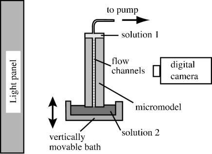
Figure 1: Experimental setup for miscible displacement measurements in 2D micromodels.

III.2 Fluid preparation and characterization

The fluids used in the experiments are shear thinning water-polymer solutions. The shear thinning fluids are solutions of $500$ to $1000$ ppm of high molecular weight scleroglucan in high purity water (Millipore - Milli-Q grade). Scleroglucan (Sanofi Bioindustries, France) is a polysaccharide with a semi rigid molecule (persistence length $\simeq 180\times 10^{-9}$ m); it has been selected because it is electrically neutral and its characteristics are therefore independent of the ion (and dye) concentration. All solutions are protected from bacterial contamination by adding $0.2$ g/l of $NaN_{3}$. In all experiments, the injected and displaced fluids are identical except for a small amount of Water Blue dye which is added to one of the solutions at a concentration of $200$ ppm by weight to allow for optical concentration measurements.
The molecular diffusion coefficient of the dye is determined independently in pure water by means of Taylor dispersion measurements performed separately in a capillary tube (the measured value of $D_{m}$ was close to $6.5\times 10^{-4}$ mm².s^-1.)
The rheological properties of the scleroglucan solutions have been characterized using a Contraves LS30 Couette rheometer with shear rates $\dot{\gamma}$ ranging from $0.016$ s^-1 up to $87$ s^-1. The rheological properties of the solutions have been verified to be constant with time within experimental error (over a time lapse of $3$ days) and identical for dyed and transparent solutions with the same polymer concentrations. The variation of the effective viscosity $\eta$ with $\dot{\gamma}$ was then adjusted by a Carreau function :

$$\eta=\frac{1}{(1+(\frac{\dot{\gamma}}{\dot{\gamma_{0}}})^{2})^{\frac{1-n}{2}}}(\eta_{0}-\eta_{\infty})+\eta_{\infty}.$$ (2)

The values of these different rheological parameters for the polymer solutions used in the present work are listed in Table 1; determining $\eta_{\infty}$ would have required values of $\dot{\gamma}$ outside the measurement range so that we assume that $\eta_{\infty}\,=\,10^{-3}$ Pa.s (the value for the solvent i.e. water). In Eq.(2), $\dot{\gamma_{0}}$ corresponds to a crossover between two regimes. On the one hand, $\dot{\gamma}<\dot{\gamma_{0}}$, the viscosity $\eta$ tends towards $\eta_{0}$, and the fluid displays a Newtonian behavior (”Newtonian plateau” regime). On the other hand, for $\dot{\gamma}\gg\dot{\gamma_{0}}$, the effective viscosity decreases with the shear rate following the power law $\eta\propto{\dot{\gamma}}^{(n-1)}$ ($n=1$ for a Newtonian fluid.) It should finally be noted that the high effective viscosity of these solutions at low shear rates avoids the appearance of buoyancy induced instabilities at low shear rates and helps stabilize the fluid displacement.

Polymer Conc.	$n$	$\dot{\gamma_{0}}$	${\eta}_{0}$
ppm		$s^{-1}$	$mPa.s$
$500$	$0.38\pm 0.04$	$0.077\pm 0.018$	$410\pm 33$
$1000$	$0.26\pm 0.02$	$0.026\pm 0.004$	$4500\pm 340$

Table 1: Rheological parameters of scleroglucan solutions used in the flow experiments.

III.3 Fluid injection and flow visualization

The model is placed vertically with its open sides horizontal : the upper side is fitted with a leak tight adapter allowing one to suck fluid upwards. The lower open side is initially slightly dipped into a bath of one of the liquids and is saturated with this fluid by pumping it slowly upwards. After switching off the pump, the bath can be lowered until it does not touch any more the model (Fig. 1). The bath is then completely emptied, refilled with the other fluid and raised to its initial position. Finally, the first fluid is sucked upwards at the upper end of the model by the syringe pump. This allows one to obtain a front of the displacing fluid which is initially perfectly straight. The lower bath rests upon computer controlled electronic scales for monitoring the amount of fluid which has entered the model. The flow rates used in the experiments correspond to mean front velocities between $0.005$ and $2.5$ mm.s^-1.
The model is illuminated from the back by an electronic light panel and images are acquired by a $12$ bits, high stability, digital camera with a $1030\times 1300$ pixels resolution and then recorded by a computer. The pixel size is $0.14$ mm or $0.4$ times the mean width of the channels: this allows one to discriminate between the various regions of the pore space. Typically $100$ images are recorded for each experimental run at time intervals from $2.5$ to $700\,s$.

III.4 Image analysis procedure

The images are then translated into maps of the relative concentration using the following procedure. First, a calibration curve is obtained from images of the model saturated with $7$ solutions of increasing dye concentration $C$ starting from zero up to the concentration used in the experiments. The logarithm $Ln(I(C)/I_{o})$ of the transmissivity is then plotted as a function of $C$; $I(C$) and $I_{o}$ are averages of the light intensity over the model and correspond respectively to dye concentrations equal to $C$ and $0$. Due to the non linear absorbance effect detwiler00 , a better fit is obtained with a third order polynomial variation of $Ln(I(C)/I_{o})$ with $C$ than with the linear dependence corresponding to Lambert’s law. This calibration is performed every time the locations of the light source and of the models are significantly changed.
For all experiments, reference images are recorded both with the micromodel initially saturated with the displaced fluid and, at long times, when it is fully saturated with the injected one. After the fluid displacement has been performed, the local concentrations are determined pixel by pixel for each image by means of the calibration curve. This operation is performed only on pixels belonging to channels; non flowing domains are not considered. Finally, maps of the local relative concentration of the two fluids are obtained by normalizing the local concentration between its values in the initial and final images.

IV Experimental results

IV.1 Qualitative observations of miscible displacements

Figure 2 compares displacement experiments realized at a same flow velocity for the two water-scleroglucan solutions.

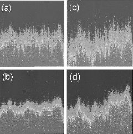
Figure 2: Relative concentration maps for experiments using water-scleroglucan solutions of respective concentrations $500$ ppm (a,b) and $1000$ ppm (c,d) for flow rate values $Q=0.075$ ml/mn (b,d) and $Q=1.5$ ml/mn (a,c). Grey levels code used in the figure : darkest shade = pure displaced fluid, intermediate - pure displacing fluid - lightest = intermediate concentrations

For a given solution, narrow structures of the front with a lateral extent of a few channel widths appear when the velocity increases and reflect local high or low velocity zones. For a same flow rate, images obtained with the two solutions are qualitatively similar: the size parallel to the flow of medium scale front structures (with a width of the order of one tenth that of the model) is however larger for the more concentrated solution both at low and high velocities.
The stability of the displacement with respect to buoyancy driven instabilities has also been verified by comparing experiments using the same pair of fluids and exchanging the injected and the displaced fluid freytes01 : no quantitative difference was measured between the two configuraton and no fingering instabilities appeared in the unstable configuration.
While fluid displacement images provide informations on the front geometry down to a fraction of the channel size, we shall see next that they also allow to determine macroscopic parameters characterizing the process.

IV.2 Quantitative dispersion measurement procedure

Quantitatively, the global displacement process is analyzed from the variations with time and distance parallel to the flow of a macroscopic concentration ${\overline{C}}(x,t)$: ${\overline{C}}$ is the average over an interval $\Delta y$ perpendicular to the flow of the local relative concentration $C$ for individual pixels located inside the pore volume. The width $\Delta y$ is large enough to average out local fluctuations and small enough avoid the influence of the side walls: ${\overline{C}}$ was found to be independent of $\Delta y$ within experimental error when these conditions are verified. Also, it will be seen below that the results are hardly different when $\Delta y$ corresponds to only one channel.

Figure 3: Normalized concentration variation ${\overline{C}}(x,t)$ as a function of time for a displacement experiment using a $500$ ppm polymer solution with $Q=3.75$ ml/mn. ${\overline{C}}$: averaging interval $\Delta y\simeq 35$ mm located in the central part of the model. Distance from inlet: $x=80$ mm. Continuous line : fit by Eq. (3).

Figure 3 displays a typical variation of ${\overline{C}}$ with time. For step-like initial concentration variations corresponding to our experiments, the solution of the convection-dispersion equation (1) is:

$${\overline{C}}=\frac{1}{2}\left[1-erf\frac{t-{\overline{t}}}{\sqrt{4\frac{D}{U^{2}}t}}\right]$$ (3)

As seen in Figure 3, a very good fit of the experimental data with this solution (continuous line) is obtained by adjusting the two parameters of the equation, namely the mean transit time $\overline{t}$ and the ratio ${D}/{U^{2}}$ ($={\overline{\Delta}t^{2}}/2\overline{t}$ where ${\overline{\Delta}t^{2}}$ is the centered second moment)

Figure 4: Variation of $\overline{t}$ with the distance $X$ (polymer concentration : $500ppm$, $Q=3.75ml/min$, $Pe=317$) for dyed fluid displacing clear fluid. Dashed line : clear fluid displacing dyed fluid. Inset : close-up at the scale of $4$ channels. Dashed line: linear regression of the variation of $\overline{t}$ with $X$.

Figure 4 displays the variation of the mean transit time $\overline{t}$ with the distance $X$ from the inlet: $\overline{t}$ increases overall linearly with distance, indicating that the mean velocity $U$ is constant and can be determined by a linear regression of the data. The inset (magnified view of the curve) shows that $\overline{t}(X)$ oscillates about the mean trend (dotted line) corresponding to the linear regression. These periodic variations are directly related to the structure of the network and will be discussed in section IV.4.

Figure 5: Variation of $D$ with the distance $X$ for dyed fluid displacing clear fluid (Polymer concentration : $500$ ppm, $Q=3.75$ ml/min, $Pe=317$.) - Inset : a close-up at the scale of $4$ channels.

Some similar features are observed on the variation of the dispersion coefficient $D$ plotted in figure 5 as a function of the distance $X$ from the injection ($D$ is computed from the value of $D/U^{2}$ given by the fit with $U$ equal to $X/{\overline{t}}$.) This time, $D(X)$ is globally constant with $X$; like $\overline{t}$, it displays periodic oscillations related to the structure of the network which will be discussed below. While these curves have been obtained for dyed fluid displacing clear fluid, comparison experiments have been realized with clear fluid displacingg dyed fluid; no systematic difference between the two sets of data was observed, confirming that there are no buoyancy driven instabilities.
The oscillations of $\overline{t}$ and $D$ as $X$ varies are closely related to mixing at the junctions and to the exchange of tracers between the transverse channels and the rest of the flow (a quantitative analyzis will be presented in section IV.4.)
The above analysis has been performed for all experiments realized with both polymer concentrations. In the following section, variations with $Pe$ of the dispersion coefficient $D$ measured in this way are discussed

IV.3 Flow velocity dependence of dispersion coefficient

Figure 6: Variation of the dispersivity $l_{d}$ (mm) with the Péclet number for experiments with water-polymer solutions : ($\square$),($\blacksquare$) : $500$ ppm concentration - ($\circ$), ($\bullet$) $1000$ ppm. Open (resp. grey) symbols : averaging interval : $35$ (resp. $0.4$) mesh sizes - Inset : variation of normalized dispersion coefficient $D/D_{m}$ as function of the Péclet number for two polymer concentration (same symbols as in main graph). Solid line : power law fit for $Pe>10$ (exponent $1.35\pm 0.03$).

The variations with the Péclet number $Pe$ of the dispersion coefficient $D$ determined as explained in the previous section are displayed in the inset of figure 6. For both polymer concentrations, $D$ always increases with $Pe$ but two different variation regimes are visible.
For $Pe\geq 10$, values of $D$ corresponding to the two polymer concentrations fall on top of each other and increase like $D\sim Pe^{\beta}$ with $\beta\simeq 1.35$. This is in good agreement with numerical simulations bruderer01 realized for a similar geometry and degree of heterogeneity (as characterized by $\sigma(a)/\bar{a}\ =\ 0.33$) and for which a power law variation with an exponent of the order of $1.3$ is also obtained. The value significantly higher than $1$ of this exponent cannot be accounted for solely by geometrical dispersion (which would give a value of $1$) even if a logarithmic correction factor such that $D~{}\propto~{}Pe~{}LogPe$ is introduced arcangelis86 . A likely hypothesis is that this variation reflects a crossover from geometrical dispersion ($D\propto Pe$) to Taylor dispersion ($D\propto Pe^{2}$): in that range of Péclet numbers, both mechanisms would then contribute to the dispersion process.
For $Pe<10$, on the contrary, values of $D$ obtained for the $1000$ ppm polymer solution are higher than those obtained with the $500$ ppm one. The variation of $D$ with $Pe$ in that range has been studied more precisely by plotting the dispersivity $l_{d}=D/U$ in the main graph of figure 6. The value of $l_{d}$ is approximately constant for $Pe\ <\ 10$ for both polymer concentrations and is larger for the $1000$ pmm solution ($l_{d}=1.71$ mm) than for the $500$ ppm one ($l_{d}=0.8$ mm). This implies that, in this range of Péclet numbers, the geometrical mechanism controls dispersion and that the corresponding dispersivity increases with the shear thinning character of the fluid (at higher $Pe$ values, $l_{d}$ is, in contrast, almost identical for the two solutions).
The values plotted in figure 6 have been obtained by averaging the concentration $C$ over $35$ channels in the direction perpendicular to the mean flow. In order to estimate the influence of the heterogeneities of the network, we performed an analysis in which the concentration $C$ is only averaged over $\Delta y=4$ pixels (or about $0.55$ mesh sizes of the lattice): the coordinates $y$ of these measurement lines are chosen so that all pixels are inside longitudinal channels or junctions and the dispersivity is determined as above.
These values of $l_{d}$ are represented as grey symbols in figure 6 and are only slightly lower than those obtained for $\Delta y=35$ mm. This shows that there are no large scale heterogeneities of the network, such as high or low permeability channels of width significantly larger than the mesh size which would increase the dispersivity.
Since all data points correspond to $Pe\geq 1$, the direct influence on longitudinal dispersion of molecular diffusion is negligible: It has however a strong indirect influence at the lower Péclet numbers investigated ($Pe\lesssim 10$). The transit time of the tracer inside the junctions or individual flow channels is then large enough so that molecular diffusion across the flow lines is significant : this influences strongly the redistribution of the incoming tracer between channels leaving each junction mourzenko02 . In the next section, we show that, in addition to the determination of macroscopic parameters like $U$, $D$ (or $l_{d}$), the concentration maps allow to investigate mixing processes at the pore scale or even below.

IV.4 Tracer exchange dynamics between transverse and longitudinal channels.

The variations with the distance $X$ from the inlet of both the mean transit time ${\overline{t}}(X)$ (Fig. 4) and the dispersion coefficient $D(X)$ (Fig. 5) display periodic oscillations about respectively an increasing linear trend and a constant value. In the following, the oscillations of $D$ will be characterized quantitatively by the difference between $D(X)$ and its mean value; the variations of ${\overline{t}}(X)$ will be characterized by its difference with the linear regression ligne over all data points reflecting the mean front velocity $U$. At a given distance $X$ the time corresponding to this regression is equal to $X/U$. The difference ${\overline{t}}(X)-X/U$ is negative when the line located at the distance $X$ from the inlet, and over which $C(X,t)$ is computed, contains only longitudinal channels parallel to the flow; it is positive when the line contains both transverse channels and junctions. Regarding $D(X)$, it is also lower than the mean value when the line $X=cst.$ contains only longitudinal channels and higher when it contains both longitudinal and transverse channels. The variations of ${\overline{t}}(X)$ reflect the different influence of longitudinal and transverse channels on transport. As already discussed in section II, in a weakly disordered square network like the present one, most convective flux is localized inside the longitudinal channels (parallel to the mean flow). The mean velocity inside them is then significantly higher than in the transverse channels and they get saturated faster with the displacing fluid. There is therefore a time lag between the saturation of the transverse and longitudinal channels at a same distance $X$ from the inlet which explains the oscillations of ${\overline{t}}(X)$ in Figure 4.
Moreover, the respective amplitudes of the successive minimas and maximas of ${\overline{t}}(X)-X/U$ are found to be almost constant from one to the other. In the following, the time lags will therefore be characterized by the respecting averages $\delta t_{l}$ and $\delta t_{jt}$ over all minimal and maximal values of ${\overline{t}}(X)-X/U$.
In the limit of a perfect mixing at the junctions ($Pe<10$), fluid particles do not retain the memory of their past trajectory (ie whether they got previously trapped inside slow transverse channels). Therefore the time lag for $X\ =\ cst$ lines containing transverse channels should reflect directly the residence time in an individual (slow) transverse channel, weighted by the volume fraction corresponding to these channels. As long as $Pe\gg 1$ and molecular diffusion is negligible, the residence time in a given channel will be inversely proportional to the local velocity; the latter is, in turn, proportional to the mean velocity $U$ as long as (as in the present case) the Reynolds number is low enough and the linear Stokes equation is approximately applicable. As a result, the local velocity in a channel is proportional to the mean velocity $U$ and the time lag $\delta t_{jt}>0$ should vary as $1/U$ (for similar reasons $\delta t_{l}<0$ should also vary as $1/U$). Figure 7 displays the variations of $\delta t_{jt}$ and $\delta t_{l}$ with $1/U$ for the two polymer solutions investigated : in both cases, the variation is indeed linear for $1/U\geq 40$ s.mm^-1 (corresponding to $Pe\leq 6$).

Figure 7: Variation of $\delta t_{l}$ (filled symbols) and $\delta t_{jt}$ (open symbols) with $1/Pe$. ($\square,\blacksquare$): experiments realized with $500$ ppm polymer solutions, ($\circ,\bullet$): $1000$ ppm. Dashed lines are guides for the eyes.

For $1/U<40$ ($Pe>6$), $\delta t_{jt}$ (resp. $\delta t_{l}$) is higher (resp. lower) than the values extrapolated from the linear trend for $1/U\geq 40$ : the transition is observed at the same mean velocity for the two solutions. This increase of the absolute values of the time lags reflects very likely the breakdown of the assumption of perfect mixing at junctions or inside individual channels : at high Péclet numbers, a solute particle may indeed flow through several junctions and channels without moving across flow lines through transverse molecular diffusion. If the lattice is weakly disordered, the solute may then remain for a longer time inside a sequence of longitudinal high velocity channels than in the case of a perfect mixing at the junctions : the corresponding value of $\delta t_{l}$ will then be lower. Similarly a solute particle may remained trapped for a longer time. in slow zones than if mixing was more effective at the junctions so that $\delta t_{jt}$ is increased.
Although the transition between the above two regimes takes place at the same Péclet number for both solutions, the absolute amplitude of the variations of $\delta t_{jt}$ and $\delta t_{l}$ with $1/U$ is significantly larger for the $1000$ ppm one. This is direct consequence of the shear thinning properties of the fluid : the effective viscosity of the solutions increases much more with the polymer concentration in slow transverse channels (where the shear rate is low) than in fast longitudinal ones : as a result, the contrast between the velocities (and therefore the residence times) in the longitudinal and transverse channels is enhanced, leading to the observed increase of $|\delta t_{jt}|$ and $|\delta t_{l}|$. This enhancement of velocity contrasts for shear thinning fluids is discussed in more detail in section V.
At the opposite limit of low velocities such that $Pe<1$ ($1/U\geq 250$ s$\times$mm^-1), longitudinal diffusive transfer becomes significant. The increase of the residence times with $1/U$ is then limited by molecular diffusion to a value of the order of a few $l^{2}/D_{m}$ ($\sim 1000$s): the variations of $\delta t_{jt}$ and $\delta t_{l}$ should then level off at high $1/U$ values. The lowest values of $Pe$ are however still too high in our experiments to observe this effect.
These results suggest therefore that the type of local observations reported here provide important informations on mixing processes at the pore scale. As pointed out recently  grubert01 ; park01 , these processes may, in turn, influence strongly mass transfer at the macroscopic scale. In a similar perspective, we shall now investigate the dependence of the geometry of the iso concentration fronts on the flow velocity and the polymer concentration. We shall also discuss their relation to local mixing in the pores.

IV.5 Geometry of tracer displacement fronts

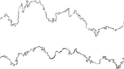
Figure 8: Isoconcentration fronts at a mean velocity $U=0.005$ mm/s ($Pe=1.3$) for polymer solutions of concentrations $1000$ ppm (upper curve) and $500$ ppm (lower curve). Mean distance of tracer from inlet : $0.5\times L$ ($L$ = model length). Flow is upward on the figure. Front widths : $\sigma\ =\ 4.5$ mm ($1000$ ppm) and $\sigma\ =\ 2.6$ mm ($500$ ppm).

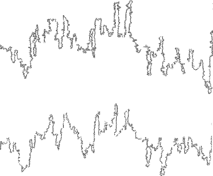
Figure 9: Isoconcentration fronts for a mean velocity $U=0.125$ mm/s ($Pe=32$) for polymer solutions of concentrations $1000$ ppm (upper curve) and $500$ ppm (lower curve). Mean distance of tracer from inlet : $0.5\times L$ ($L$ = model length). Flow is upward on the figure. Front widths $\sigma\ =\ 6.1$ mm ($1000$ ppm) and $\sigma\ =\ 4.6$ mm ($500$ ppm).

In the present experiments, the pixel size in the concentration maps is $0.4$ times the mean channel width. This allows for a study of the tracer distribution in the mixing zone at length scales varying from the size of the network down to a fraction of the pore size. For practical reasons, we shall not use the full spatial concentration distribution in the following analysis : we chose instead to characterize its spatial heterogeneity by the isoconcentration lines $c=0.5$, which are assumed to reflect the displacement front geometry: examples of such fronts determined by a thresholding procedure are displayed in figures 8 and 9 for Péclet numbers $Pe$ respectively equal to $1.3$ and $32$.
The width of the front parallel to the mean flow is larger for the more concentrated solution and it increases with the Péclet number. Also, at high $Pe$ values, large spikes are visible while the front is relatively smooth at lower ones. In spite of these differences, the main geometrical features of the front are similar: large peaks and troughs are generally located at the same points for different flow velocities and polymer concentrations. This confirms that irregularities of the front structure are associated to deterministic features of the velocity field and not to uncontrolled imperfections of the injection.
Quantitatively, the effective width of the front parallel to the flow is characterized in the following by the standard deviation $\sigma(\bar{x})$ of the distance $x$ of its points from the inlet: $\sigma(\bar{x})$ satisfies $\sigma(\bar{x})=<(\bar{x}-x(y))^{2}>^{1/2}$ in which $\bar{x}$ is the mean value of $x$. In figures 8 and 9, $\bar{x}$ is equal to half the length of the model and the values of $\sigma$ corresponding to the curves displayed are listed in the captions.

Figure 10: Effective front width $\sigma$ as a function of the mean front velocity $U$ (mm/s) for a mean distance ${\bar{x}}=0.5\times L$ and polymer concentrations equal to $1000$ ppm ($\circ$) and $500$ ppm ($\square$). Solid (resp. dotted) lines : fit of the experimental data for a $1000$ ppm (resp. $500$ ppm) polymer solution by equation $\sigma=a+b\,log(U)$ with $a=6.9\pm 0.1$ and $b=0.4\pm 0.05$ (resp. $a=6.2\pm 0.2$ and $b=0.5\pm 0.1$.

Figure 10 displays the variation of $\sigma$ as a function of the mean flow velocity $U$ for ${\bar{x}}\ =\ L/2$. For both solutions, the width $\sigma$ increases logarithmically with $U$: the value of $\sigma$ is larger for the $1000$ ppm solution while the slope of its variation with $U$ in figure 10 is slightly lower.
The values of $\sigma$ are different for the two solutions because the effective viscosity decreases faster with the velocity gradients for the $1000$ ppm solution than for the $500$ ppm one. The ratio between the effective viscosities, and therefore the velocities in the longitudinal and transverse channels is therefore higher and the front width which is directly related to this ratio increases.
The second major feature of the above results at high velocities is the large amplitude of the peaks and troughs observed on the front while they are smaller and narrower at lower velocities. This, too, may be explained by the reduced tracer mixing at junctions at high Péclet numbers (section IV.4) : solute remaining for a long distance inside longitudinal, high velocity, channels will contribute to the spikes while that moving through a sequence of slow lateral channels will contribute to the troughs. At lower Péclet numbers, mixing is more efficient and solute particules sample more effectively the velocity distribution: this reduces the dispersion of the transit times and, therefore the amplitude of the peaks and troughs.

V Discussion and conclusions

The local analysis of the transit times and of the front geometry have therefore provided important informations on mixing inside junctions and flow channels and on its dependence on the Péclet number. This information greatly helps one to interprete the macroscopic dispersivity measurements of section IV.2. Some of the features observed are specific to 2D systems while others can occur in usual 3D media.
At low Péclet numbers (typically $Pe\ \leq\ 10$), the dispersivity $l_{d}$ remains constant with $Pe$ and is lower for the $500$ ppm polymer solution than for the $1000$ ppm one. In sections IV.4 and IV.5, we have seen that, in this regime, transverse mixing in junctions and channels is very effective so that the correlation length of the motion of solute particles is of the order of the length $l$ of individual channels. As a result, this motion may be described as a sequence of random steps of varying durations and directions inside the medium; this is the geometrical dispersion regime discussed in section II and for which $D\propto Pe$ ($l_{d}\ =\ cst.$).
In this regime, the factor of two difference of the dispersivities for $500$ and $1000$ ppm solutions is likely due to enhanced velocity contrasts between the fast and slow flow regions. It is known, for instance shah95 , that the mean flow velocity inside a cylindrical channel under a given pressure gradient varies as the square of the radius $a$ for a Newtonian fluid and as $a^{1+\frac{1}{n}}$ for a shear thinning fluid verifying equation (2). Let us assume that the pressure gradient between the ends of flow channels in parallel is constant. If $\sigma(a)\ll\bar{a}$, the standard deviation $\delta U$ of the mean velocities in the different channels should scale like :

$$\frac{\delta U}{U}\sim\frac{1+n}{n}\frac{\sigma(a)}{\bar{a}},$$ (4)

where $\sigma(a)/\bar{a}$ is the normalized standard deviation of the channel aperture (see section III.1). Still using the same simplistic approach, the typical standard deviation $\delta t$ of the transit time along a channel of length $l=0.67$ mm should be $l/\delta U$. Estimating the dispersion coefficient $D$ from the relation $D\sim l^{2}/\delta t$ provides the order of magnitude of the dispersivity :

$$l_{d}\ \sim\ \frac{n+1}{n}\frac{\sigma_{a}}{a}\ l$$ (5)

Since $n$ decreases with the polymer concentration, $l_{d}$ should therefore increase for a fixed aperture fluctuation $\sigma(a)/a$. Using in equation (5) the values of $l$, $\sigma(a)/a$ and $n$ corresponding to the present experiments (table 1) leads to $l_{d}\simeq 0.7$ mm and $1$ mm respectively for the $500$ ppm and $1000$ ppm solutions. These estimations are close to the experimental values $l_{d}\ =\ 0.8$ mm and $1.7$ mm reported in section IV.3 for the same solutions (figure 6). The difference may be due to the assumption of identical pressure gradients on different parallel channels used to obtain equations 4 and 5.
At higher Péclet numbers $Pe\ >\ 10$, $l_{d}$ is no longer constant but increases with $Pe$. This reflects the transition towards a second dispersion regime in which mixing is less effective. One must then take into account the stretching of dye parallel to the flow by local velocity gradients in the flow section (dye moves slower in the vicinity of the walls than in the center of the channels). This stretching effect, is balanced by transverse molecular diffusion, resulting a Taylor-like dispersion mechanism (section II). This effect is made significant by the increase with $Pe$ of the correlation length of dye transport along chains of flow channels parallel to the mean flow discussed above in sections IV.4 and IV.5.
The effect of the local velocity gradients is also enhanced by the specific topology of $2D$ micromodels. The upper and lower walls are indeed continuous and some flow lines remain close to them over their full length: as in Taylor dispersion, slow solute particles near these walls may only move away from them through molecular diffusion. Similarly, fast moving particles half way between the walls can only reach them through transverse molecular diffusion. The large correlation length of these velocity contrasts also results in Taylor-like dispersion effects.
Yet, the influence of the disorder of the medium cannot be completely neglected (since some tracer always moves into lower velocity transverse channels): the global dispersion results therefore from the combined effects of geometrical and Taylor dispersion. As a result, the macroscopic dispersion coefficient $D$ follows in this regime a power law $D\propto Pe^{\beta}$ of the Péclet number with an exponent $\beta\simeq 1.3$ intermediate between the values $1$ and $2$ corresponding respectively to Taylor and geometrical dispersion.
Regarding the influence of the shear thinning properties, increasing the polymer concentration enhances velocity contrasts between different flow channels while it flattens the velocity profile in individual channels. The first effect increases geometrical dispersion and is indeed observed at low Péclet numbers. The second reduces Taylor dispersion : this explains why, at higher $Pe$ values, the values of $l_{d}$ for the two polymer solutions are similar when the influence of Taylor dispersion is large.
To conclude, the dispersion measurements reported in the present work for transparent micromodels provide significant novel informations on the influence of the flow velocity and fluid rheology on miscible displacements in porous media. Quantitative high resolution optical measurements have allowed for thorough studies over a broad range of length scales: it has in particular been possible in the same experiment both to determine macroscopic parameters such as the effective dispersivity and to analyse at the pore scale the dynamics of concentration variations.
In particular, the local analysis of the time lag between the invasions of longitudinal and transverse channels of the model has allowed us to relate the transition between two dispersion regimes for $Pe\simeq 10$ to variations of mixing in channel junctions. The variations of small scale structures of the displacement front with the Péclet number and the polymer concentration also provides informations on the spatial correlation of transport at the local scale.
In the future, investigation of these effects at still higher resolutions should allow for detailed direct studies of mixing and flow patterns right inside individual flow channels and their junctions.

- (1) J. Bear, “Dynamics of Fluids in Porous Media”, Elsevier Publishing Co., New York (1972).
- (2) F.A.L. Dullien, “Porous Media, Fluid Transport and Pore Structure”, 2nd edition, Academic Press, New York (1991).
- (3) E. Charlaix, J.P. Hulin, C. Leroy and C. Zarcone. “Experimental study of tracer dispersion in flow through two-dimensional networks of etched capillaries.” J. Phys. D: Appl. Phys. 21, 1727 (1988).
- (4) P.Z. Wong, Ed. “Methods in the physics of porous media.”, Experimental methods in the physical sciences 35, Academic Press, London (1999).
- (5) R. Lenormand, C. Zarcone and A. Sarr. “Mechanism of the displacement of one fluid by another in a network of capillary ducts,” J. Fluid Mech. 135, 337 (1983).
- (6) A. Birovljev, K. J. Måløy, J. Feder, and T. Jøssang. “Scaling structure of tracer dispersion fronts in porous media.” Phys. Rev. E 49, 5431 (1994).
- (7) D. Grubert. Effective dispersivities for a two-dimensional periodic fracture network by a continuous time random walk analysis of single-intersection simulations. Water Resour. Res. 37, 41 (2001).
- (8) Y. Park, J.R. de Dreuzy, K. Lee and B. Berkowitz. “Transport and intersection mixing in random fracture networks with power law length distributions.” Water Resour. Res. 37, 2493 (2001).
- (9) K.S. Sorbie, P.J. Clifford and E.R.W. Jones, “The rheology of pseudoplastic fluids in porous media using network modeling.” J. Colloid Interf. Sci. 130, 508 (1989).
- (10) A. Paterson, A. D’Onofrio, C. Allain, J.P. Hulin, M. Rosen and C. Gauthier. “Tracer dispersion in a polymer solution flowing through a double porosity porous medium.” J. Phys. II France 6, 1639 (1996).
- (11) M.A. Freytes, A. d’Onofrio, M. Rosen, C. Allain, J.P. Hulin. “Gravity driven instabilities in miscible non Newtonian fluid displacements in porous media.” Physica A 290, 286 (2001).
- (12) V.V. Mourzenko, F. Yousefian, B. Kolbah, J.F. Thovert and P.M. and Adler, “Solute transport at fracture intersections.” Water Resour. Res. 38, 1000 (2002).
- (13) B. Berkowitz, C. Naumann and L. Smith, “Mass transfert at fracture intersections: An evaluation of mixing models.” Water Resour. Res. 30, 1765 (1994).
- (14) G.I. Taylor, “Dispersion of soluble matter in solvent flowing slowly through a tube.” Proc. R. Soc. London A 219, 186 (1953).
- (15) R. Aris, “On the dispersion of a solute in a fluid flowing through a tube.” Proc. R. Soc. London A 253, 67 (1956).
- (16) M. Vartuli, J.P. Hulin and G. Daccord, “Taylor disper sion in a polymer solution flowing in a capillary tube.” AIChE J. 41, 1622 (1995).
- (17) C.B. Shah and Y.C. Yortsos, “Aspects of flow of power-law fluids in porous media.” AIChE J. 41, 1099 (1995).
- (18) A. Fadili, P. Tardyand and A. Pearson, “A 3D filtration law for power-law fluids in heterogeneous porous media.” J. Non-Newtonian Fluid Mech. 106, 121 (2002).
- (19) C. Bruderer and Y. Bernabé, “Network modeling of dispersion: Transition from Taylor dispersion in homogeneous networks to mechanical dispersion in very heterogeneous ones.” Water Resour. Res. 37, 897 (2001).
- (20) R.L. Detwiler, H. Rajaram and R.J. Glass, “Solute transport in variable-aperture fractures: An investigation of the relative importance of Taylor dispersion and macrodispersion.” Water Resour. Res. 36, 1611 (2000).
- (21) de Arcangelis L., J. Koplik, D. Redner and D. Wilkinson, Hydrodynamic dispersion in network of porous media, Phys. Rev. Lett., (1986) 57, 996–999.