Statistical analysis of coherent structures in transitional pipe flow
Abstract
Numerical and experimental studies of transitional pipe flow have shown the prevalence of coherent flow structures that are dominated by downstream vortices. They attract special attention because they contribute predominantly to the increase of the Reynolds stresses in turbulent flow. In the present study we introduce a convenient detector for these coherent states, calculate the fraction of time the structures appear in the flow, and present a Markov model for the transition between the structures. The fraction of states that show vortical structures exceeds 24% for a Reynolds number of about , and it decreases to about 20% for . The Markov model for the transition between these states is in good agreement with the observed fraction of states, and in reasonable agreement with the prediction for their persistence. It provides insight into dominant qualitative changes of the flow when increasing the Reynolds number.
pacs:
47.27.Cn, 47.27.eb, 47.27.nf, 47.27.DeI Introduction
The visualization of turbulent flows and boundary layers via sophisticated experimental methods like particle imaging velocimetry has led to the identification of a rich variety of prominent coherent structures, such as waves, streaks, hairpin vortices and lambda vorticesRobinson (1991); Holmes et al. (1998); Podvin and Lumley (1998); Panton (2001). These extended coherent structures significantly influence large scale momentum transport and hence Reynolds stresses. As a consequence, they figure prominently in turbulence research.
Studies on internal flows in confined geometries have highlighted the dominant role of structures containing pronounced downstream vortices and have led to the proposal of a three-step self regenerating mechanism for turbulence Boberg and Brosa (1988); Jimenez and Moin (1991); Trefethen et al. (1993); Hamilton et al. (1995); Waleffe (1995, 1997, 1998); Grossmann (2000); Jimenez (2003). Downstream vortices transport liquid across the mean shear gradient and create regions of fast or slow moving fluid, so-called high- and low-speed streaks. The streaks generated by this lift-up process become unstable to the formation of normal vortices, and through a nonlinear interaction mechanism the latter feed their energy back to downstream vortices. This closed self-regeneration mechanism appears to be a generic dynamical feature of turbulent shear flows. The process was identified in direct numerical simulations of plane Couette flow in narrow cells where transverse modulations are constrained Jimenez and Moin (1991); Hamilton et al. (1995); Jimenez (2003), but it can also be detected in time-correlation functions in fully turbulent flows Jachens et al. (2006).
In its purest form this self-regenerating cycle gives rise to a periodic solution to the equations of motion. However, in most coherent structures the flow is not strictly periodic and always perturbed by background fluctuations. Examples of exact coherent states have been given in simple models, where they correspond to periodic orbits Moehlis et al. (2004, 2005); Smith et al. (2005a, b), and, in the full flow, through the numerical identification of exact coherent states in channel flows Nagata (1990); Ehrenstein and Koch (1991); Schmiegel and Eckhardt (1997); Nagata (1997); Clever and Busse (1997); Waleffe (1998, 2001); Kawahara and Kida (2001); Eckhardt et al. (2002) and travelling waves in pipe flow Faisst and Eckhardt (2003); Waleffe (2003); Wedin and Kerswell (2004). In all these cases, the coherent structures are dominated by pairs of counter-rotating downstream vortices and associated streaks which are regularly arranged in azimuthal direction. The flow fields are invariant under discrete rotations around the pipe axis.
Since all exact coherent states constructed so far are linearly unstable it came as a surprise that they could be directly observed in experiments Hof et al. (2004). In this work we follow up on this experimental observation with a study of the appearance and persistence of these structures in numerical simulations of pipe flow. In particular, we show how they can be detected, how frequently they appear, and how long they persist.
The travelling waves observed in pipe flow are of particular interest because they are believed to form a backbone for the turbulent dynamics near the onset of turbulence. Since the laminar profile in these flows is linearly stable for all Reynolds numbers Davey and Drazin (1969); Salwen et al. (1980); Patera and Orszag (1981); Drazin and Reid (1981, 2nd edition 2004); Brosa (1986, 1989); Herron (1991); Meseguer and Trefethen (2003) the transition cannot proceed through states bifurcating from the laminar profile. The turbulent motion which in many pipe-flow experiments is observed for Reynolds numbers beyond about 2000, must hence arise via a nonlinear transition scenario Boberg and Brosa (1988); Waleffe (1995); Brosa and Grossmann (1999); Eckhardt and Mersmann (1999); Faisst and Eckhardt (2004); Eckhardt et al. (submitted). The travelling waves are then the simplest persistent nonlinear structures around which the turbulent dynamics can form. Together with their stable and unstable manifolds they can give rise to the basic building blocks of chaotic dynamics, such as hyperbolic tangles and Smale horseshoes. While it is unlikely that one will be able to identify an individual travelling wave in a time series, it is possible to identify a visit to their neighborhood, as identified by the appearance of similar structures in the flow.
In the present paper we propose a way to detect the visits to the neighborhoods of coherent states, and use it to infer information about the structures underlying turbulence. To distinguish different parts of state space and different flow topologies, we introduce projections onto lower dimensional subspaces that capture salient features of classes of coherent states, and study the recurrences to these subspaces: This is weaker than identifying individual travelling waves but sufficient to discriminate between various flow regimes. On the technical side, the reduction in resolution also lowers the requirements on the length of the time traces and helps to improve the statistical significance.
The outline of the paper is as follows. In Sect. II we briefly describe the spectral code underlying the simulation of the flow. In Sect. III we describe the projection used to detect and characterize the coherent structures in direct numerical simulations of pipe flow close to the threshold of turbulence. In Sect. IV we analyst the statistics of the occurrence of coherent structures, and in Sect. V we explore their physical properties. The paper closes with a discussion and outlook in Sect. VI.
II Simulation of pipe flow
We consider an incompressible Newtonian liquid in a pipe of circular cross section subject to no-slip boundary conditions at the walls. The flow is forced by a uniform pressure gradient which is adjusted to keep the flux constant at any instant of time Draad et al. (1998); Darbyshire and Mullin (1995); Hof et al. (2004). In other words the integrated volume flux through a cross section of the pipe is constant, and the Reynolds number
| (1) |
is externally controlled in order to be independent of the flow state of the liquid. Here denotes the mean downstream velocity, is the pipe radius and the kinematic viscosity of the liquid. In our simulations the pipe is long, and we use periodic boundary conditions in the downstream direction: physically, this corresponds to a numerical representation of the interior of a turbulent patch.
The Navier-Stokes equations are written in cylindrical coordinates and solved with a pseudo-spectral scheme. In doing so dimensionless units where lengths are measured in units of the radius of the pipe and velocities in units of twice the mean downstream velocity (i.e., the centerline velocity of the equivalent parabolic laminar profile) are used. Time is measured in units of .
All three components of the velocity field are decomposed into Fourier modes in azimuthal and downstream direction. Chebyshev polynomials are used for expansion in radial direction. The velocity field is thus written as
| (2) |
Here the spectral basis functions are
| (3) |
where denotes the normalized Chebyshev polynomial Abramowitz and Stegun (1984); Canuto et al. (1988), and . In physical collocation space the velocity fields are represented by the values of the fields at the corresponding Gauss-Lobatto grid points.
A 4th-5th-order Runge-Kutta-Fehlberg scheme with adaptive step-size control is used to evolve the solution in time Press et al. (1992, reprinted with corr. 2003), and the action of the Navier-Stokes operator is computed via a pseudo-spectral scheme. The transformation between spectral and physical space required by the pseudo-spectral scheme is performed by FFT-based routines. Constraints (incompressibility, regularity and analyticity) as well as no-slip boundary conditions are enforced by a Lagrangian projection mechanism Schneider (2005).
The simulations presented in this work are carried out with Fourier modes in azimuthal and Fourier modes in downstream direction, where . Consequently, we consider up to Fourier modes in azimuthal and up to in the downstream direction. Chebyshev polynomials are used for the expansion in the radial direction, adding up to components.
 |
(a)
 (b)
(b)
|
III Detection of Coherent Structures
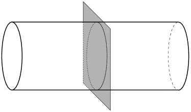
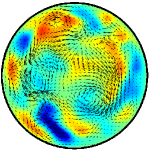
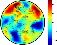
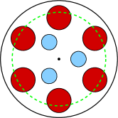
The travelling waves Faisst and Eckhardt (2003); Wedin and Kerswell (2004) we want to detect are dominated by vortices aligned along the axis, and corresponding streaks in the downstream velocity components. The downstream vortices and streaks are most prominent in cross sections of the pipe perpendicular to the axis. As in the experiments Hof et al. (2004), where stereoscopic particle image velocimetry was used to extract the velocity fields, we will focus on the velocity fields in cross sections perpendicular to the pipe axis (Fig. 1). For the travelling waves it makes no difference whether we focus on one cross section and follow the time evolution or whether we freeze the flow at one instance of time and move the cross section along the axis. The same applies for a transient appearance of these structures: in a fixed cross section they will come and go, and in a frozen flow they would be present in some regions along the axis and absent in others. In the analysis presented below we work, as in the experiments, with the time evolution in cross sections at a fixed position in the lab frame. Typical examples of cross sections with high- and low-speed streaks, i.e., of regions of high and low downstream velocity, are shown in Fig. 2. The structures are best visible when a reference profile is subtracted. In previous works Hof et al. (2004) the laminar profile with equal mean velocity was subtracted. Here we use the mean turbulent profile. It is obtained as the average over azimuthal angle and time of the downstream velocity at a fixed radius.
III.1 Characterizing the symmetry of coherent states
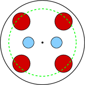
As mentioned in the introduction the coherent travelling waves identified so far have highly symmetric arrangements of vortex pairs. By transporting fast liquid from the center to the walls and slow liquid from the wall to the center region, these pairs of vortices generate elongated regions of fast and slow moving liquid. We therefore focus on the appearance of symmetric arrangements of high- and low-speed streaks schematically indicated in Fig. 3. The travelling waves also show that the high-speed streaks close to the walls are fairly stable and do not move much in the azimuthal direction over one period. This simplifies their detection amidst the fluctuations of the total velocity field.
The rotational symmetry of the pipe entails that patterns should be considered identical when they only differ by a global rotation around the pipe axis. A detector for coherent states should take this into account and be invariant under global rotations. We therefore suggest to use an azimuthal correlation of the downstream velocity at a chosen radius and axial position ,
| (4) |
where denotes averaging over . By a straightforward calculation one verifies that this correlation function is invariant under global rotations. Moreover, it reliably uncovers periodic structures in the azimuthal direction.
|
Whenever the system approaches a coherent state showing high-speed streaks close to the wall, the correlation function shows peaks separated by an angular displacement . In particular, the four-fold structure of the downstream velocity field, Fig. 2b results in a clear four-fold structure of the correlation function, which is shown in Fig. LABEL:fig:correlationsa. In addition to the autocorrelation peak at the correlation function shows peaks at . Similarly, a flow with a three-fold symmetry gives rise to peaks at (cf. Fig. LABEL:fig:correlationsb).
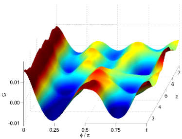 |
By following in time one can detect the lifetimes of structures, their decay, and the subsequent emergence of new patterns. An example is given in Fig. 5, which shows the decay of a four-streak state and the emergence of a six-streak state within about pipe radius.
III.2 Automated structure detection
The correlation function signals the proximity of the flow to a coherent state by evenly spaced peaks. Its derivatives highlight both minima and maxima of the correlation function (see Fig. 6) and emphasize flow structures of comparable (azimuthal) streak gradients. Since is an even function in , its derivative is odd. It should have an substantial overlap with the sine-function of the appropriate periodicity. In order to automatically detect evenly spaced maxima and in order to count their number we therefore define the scalar measures via a scalar product of the derivative of the correlation function and 111The scalar measure can be effectively computed as . ,
| (5) |
This reduction of information to a scalar quantity contains one parameter, the radius at which the correlation functions are determined. For the Reynolds numbers considered here we find to be convenient. At this radius, which is indicated by a dashed green line in Fig. 3, the coherent structures under investigation show a pronounced regular arrangement of high-speed streaks.
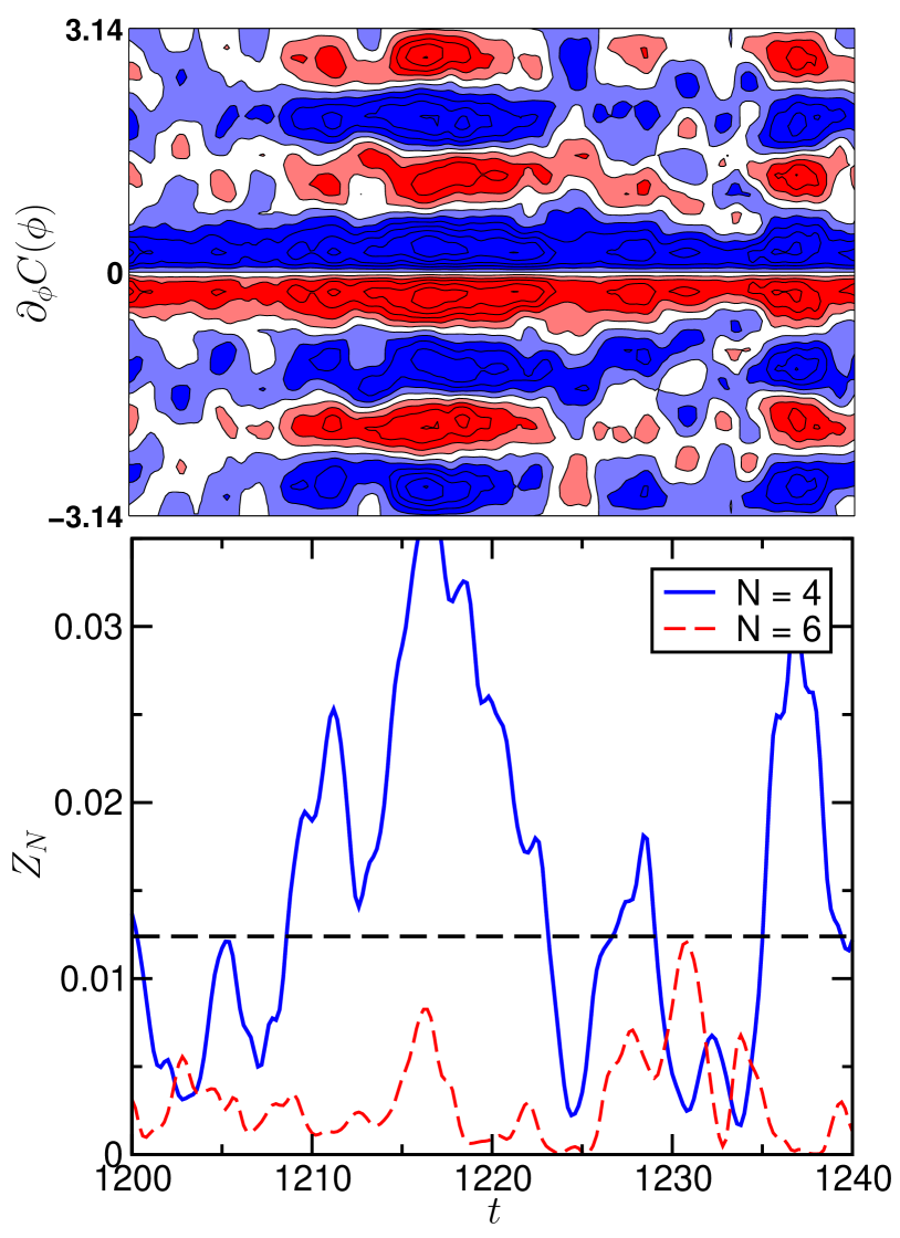
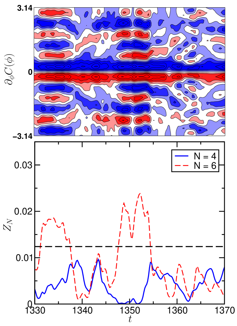
By following time traces of for different we can study the prevalence of structures of certain multiplicity and the transitions between them. Examples are given in Fig. 6. The top frames show , the derivative of the azimuthal correlator with respect to the angular coordinate , as a function of the azimuthal coordinate and the time . The four-fold structures have eight zeros in their derivative (from four maxima and four minima), and the six-fold structures have twelve zeros. Parallel nodal lines indicate the presence of these structures for times of about ten natural time units.
The lower frames in Fig. 6 show the time evolution of the corresponding scalar projectors . The indicator shows pronounced peaks when the four-fold symmetric patterns are observed in the correlation function and peaks when the six-fold structures appear; conversely, one is small when the other one is large. One also notes considerable fluctuations due to the residual background turbulence. In general, values of smaller than about cannot be considered significant indicators of a structure and belong to background fluctuations. On the other hand, comparison of the top and bottom frames in Fig. 6 suggests that a threshold signifies the presence of coherent structures with -fold symmetry.
Armed with this threshold, we collapse the scalar time series for to a single discrete indicator, , which assigns to a cross section at time the number of symmetric streaks and corresponding vortices it contains. takes the values , , , where is assigned to cases where all remain below the threshold. The maximal value is an empirical limit, in that states with eight or more vortices were rarely realized.
(a)
 (b)
(b)
 (c)
(c)
|
IV Statistical analysis of the time series
Based on the time series we now explore the statistical properties of the occurrence of coherent structures in pipe flow. The aim of this statistical analysis is twofold: we want to see how frequently structures of a certain multiplicity are present and we want to study the extend to which a Markov approximation can describe the switching between states.
IV.1 Probability distribution of coherent states
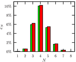
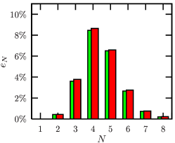
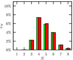
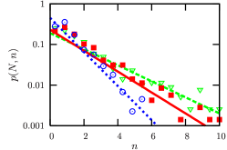
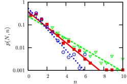
Fig. 7 shows the probabilities of detecting a coherent state of -fold symmetry in time series taken at different Reynolds numbers close to the transition to turbulence. For about % of all cross sections fall into the categories , , , and . For , the fraction decreases slightly to about . This high fraction explains the ease with which coherent structures were picked out of experimental cross sections Hof et al. (2004), and underlines their significance as building blocks of the turbulence in the transition region.
With increasing Reynolds number the weight of states with large increases. These structures are much closer to the walls where they give rise to steeper gradients in radial and azimuthal direction and consequently larger friction. As these structures have more spatial degrees of freedom, it is less likely that they appear in perfect symmetry. Hence, their correlators have smaller amplitudes, and it would be interesting in forthcoming work to probe for the structures with a localized correlator.
(a)
 (b)
(b)
 (c)
(c)
|
IV.2 Markov model for transitions
The typical persistence time of a pattern in Fig. 6 is about to time units, and the transition between the four-streak and six-streak state shown in Fig. 5 takes about one time unit. When discretizing time in order to describe the transitions between different patterns, the sampling time scale should therefore not be much longer than about . Otherwise one misses states. On the other hand, if the time steps are much shorter than unity, one begins to probe the continuity of the time evolution. As representative examples in this interval we explored the discrete dynamics of discretized time sequences with a time spacing of and of . Since different lead to results which cannot be distinguished within our error margins, we will in the following present data for only.
By considering the underlying flow at multiples of the time unit its continuous dynamics is transformed into a discrete time-series. The conditional probability that one encounters an -streak state in the following snapshot, when currently facing an -streak state defines a transition matrix . Its indices and take the values (when there is no streak), and when exceeds its threshold value. For the Reynolds number we find
| (6) |
The columns of the matrices add up to because each state has to go to one of the eight admissible states in the next time step,
| (7) |
More than independent snapshots ( for , and more than snapshots at the higher and ) were analyzed in our statistics. For the lowest Reynolds number the class is observed only a single time, and it immediately relaxed into the state (cf. rightmost column of ). Despite its rare occurrence, the state is included in the analysis because its statistical weight increases with Reynolds number: It reaches at .
IV.3 Invariant distribution and life time of coherent states
To check that the Markovian dynamics generated by the transition matrices faithfully represents the continuous dynamics, we first calculate the invariant probability distribution , defined as the eigenvector to the eigenvalue 1, i.e.
| (8) |
Fig. 7 shows that the faithfully reproduce the relative frequencies in the original data. A comparison of the histograms for the different shows that the number of visited coherent states and the complexity of the resulting flow patterns increase when the Reynolds number increases.
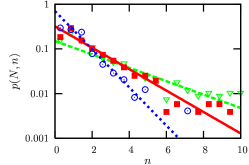
Except for the highest transfer probabilities in each column appear along the diagonal of . These elements describe the persistence of flow patters from time step to time step. Therefore, the probability density function to observe the pattern for consecutive time steps scales like
| (9) |
Fig. 8 shows data for the life time calculated from direct numerical simulation of the flow, together with the prediction from the Markov model, which is shown as straight lines in the semilogarithmic plot of lifetimes. Since long persistence times are exponentially suppressed this comparison requires very long time series to check the prediction with reasonable statistical accuracy. Within these limitations there is a very good agreement between the data and the prediction.
V Physical properties of detected states
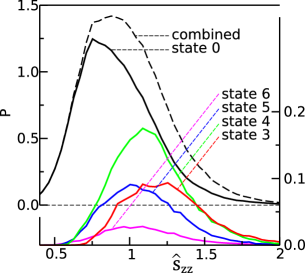
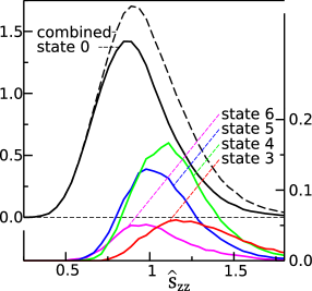
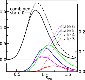
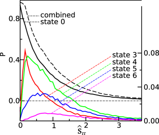
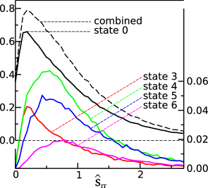
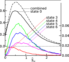
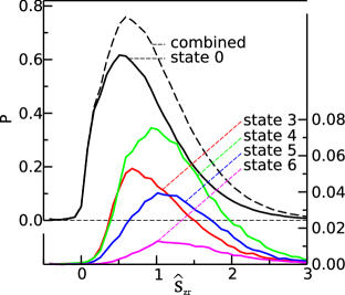
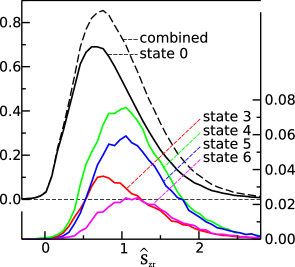
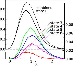
The different flow patterns also affect the different velocity and fluctuation statistics. As examples we consider the Reynolds stresses , and . Taking averages over , but not over time, provides probability distribution function (pdf) of temporal variations of these quantities (dashed lines in Fig. 9 tagged as combined), as well as conditional pdfs referring to states with a fixed number of streaks (solid lines tagged as state 3…state 6) and the turbulent unstructured state (solid lines tagged as state 0). The overall pdf can thus be decomposed into contributions of the previously discussed high-symmetry coherent states and a turbulent remainder (state 0). To emphasize the role played by the coherent states in changing the shape of the distribution of the considered component of the Reynolds stress the abscissa is always normalized to its overall temporal average. For instance, is normalized by its average , and the resulting normalized stress is denoted . By definition the mean of the distribution is therefore unity. However, the conditional pdfs for specific states will in general have means different from one. If the mean is larger than one, the state shows — on average — larger stress components than the temporal average value of the component. Table 1 lists both the absolute and the normalized mean values of all pdfs shown in Fig. 9.
| tot | |||||||
|---|---|---|---|---|---|---|---|
| 0 | |||||||
| 3 | |||||||
| 4 | |||||||
| 5 | |||||||
| 6 | |||||||
| tot | |||||||
| 0 | |||||||
| 3 | |||||||
| 4 | |||||||
| 5 | |||||||
| 6 | |||||||
| tot | |||||||
| 0 | |||||||
| 3 | |||||||
| 4 | |||||||
| 5 | |||||||
| 6 | |||||||
V.1 PDFs at fixed
From a physical point of view the interest of the decompositions of the total pdf into conditional ones for turbulent and individual coherent states lies in the insight it gives into how the coherent states contribute to the exceptional statistics of fluctuations in turbulent flow. We first consider the decomposition of the pdfs at fixed , i.e., we discuss the trends in the mean of the data shown in individual panels of Fig. 9.
On the average the detected coherent states generate much stronger Reynolds stresses than those found for the unstructured turbulent state . Consequently the coherent states shift the means and the maxima of the combined pdf to slightly larger values. Compared to the pdf of state 0 (dashed black line) the coherent states add a fat tail to the combined pdf (black solid line) on the side of larger values of the stresses. In order to gain insight into the mutual importance of the different states we discuss the trends in the mean and maxima as a function of the number of streaks .
The normalized stress characterizes the intensity of streak structures in the flow field by estimating their downstream velocity. The maxima and mean values of its pdf decrease in the order , , and . This can be interpreted as follows: The product of typical gradients of with the length scale over which the gradients persist is of the order of magnitude of the typical velocity fluctuation in downstream direction. Consequently, the azimuthal components of the gradients of are of the same order of magnitude in all coherent states, and their typical length scale decreases like .
The radial component measures the typical fluctuations of the radial velocity component, i.e., it characterizes the strength of the vortices. For this stress there also is a clear trend in the position of the maxima and mean values with , but with the sequence reversed: the highest value for the maximum appears for , and it decreases towards . This finding suggests that stronger vortices are needed to maintain the smaller streaks in coherent states with larger .
From a physical point of view the Reynolds stress is the most interesting of the three quantities. After all, it reflects the strength of the radial momentum transport. Hence it provides direct insight in the friction factor in the turbulent flow Eggels et al. (1994), and it also immediately reflects the role of the coherent states in the flattening of the laminar flow profile in radial direction. In view of the opposite scaling of the radial and axial velocity components observed in and , respectively, its dependence results from a most subtle balance. Indeed, the counteracting trends almost cancel, leaving only a very weak decrease in the position of the maxima in the sequence , , and .
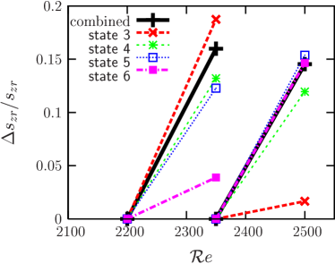 |
V.2 Drift of the mean with
In order to explore how the components of the Reynolds stress change with Reynolds number, and which physical effects generate the observed trends, one observes that the mean of a combined pdf with , , and is the weighted average of the means of the conditional distributions ,
In Fig. 9 the conditional pdfs are plotted together with their sum for , , and , respectively, and the abscissa is scaled such that . The shift in the mean of therefore arises as an average of the distance of the mean from unity with weights previously discussed in the framework of the Markov model (cf. Fig. 7). There are two physical effects underlying the observed changes in the statistics with : (1) the change of the mean of conditional pdfs of the different states, and (2) the change in the statistical weights of the states. We will disentangle these contributions now for the physically most interesting case of .
Both visual inspection of the conditional pdf in Fig. 9 (bottom row), and the values of the normalized mean values in Table 1 show that there only is a slight drift of the coherent states’ pdfs with . In contrast, as observed upon discussing Fig. 7 their weights show pronounced changes. The nontrivial evolution of their weights with suggests that the coherent states contribute to the change of the overall mean mainly by the change of their statistical weights . This becomes particularly clear when plotting the relative change of the position of the mean when increasing from to and from to , respectively (Fig. 10). In the first interval this change is dominated by the one of state 3 while state 6 hardly contributes, and in the latter interval these two states take just the opposite roles.
We thus conclude that our statistical analysis allows us to identify the contributions of individual coherent states to the anomalous statistics of turbulent pipe flow, and to disentangle the changes with into changes of the statistical weights of the states, and the comparatively smaller ones due to the -dependence of the properties of individual states. One can interpret these findings as a hint that turbulent transients close to are dominantly influenced by coherent states with only few streaks. In contrast, at higher successively more coherent states with larger number of streaks affect the time series.
VI Discussion
In this section we want to summarize the results from the present simulation of pipe flow and point to the parts that could be useful in analyzing other shear flows as well.
The automatic detection algorithm for coherent states, which was first used in Hof et al. (2004) and was expanded on here, is fairly robust. It can be generalized to other flows as well. The algorithm systematically searches for structures that show a symmetric azimuthal arrangement of high-speed streaks along the wall which is topologically very similar to the one observed in exact coherent states reported in Faisst and Eckhardt (2003); Wedin and Kerswell (2004); Hof et al. (2004). The detection is based on a Fourier-mode decomposition of the radial velocity. Because the detected states have the same symmetry structure also in the other components of the velocity field, the results should be robust against details of the implementation of the detector. Different projectors constructed along the line outlined in Sect. III should lead to identical results. For extensions to larger it might, however, be valuable to consider extensions to asymmetric expansions of the flow field, e.g. by using wavelet Daubechies (1990); Gershenfeld (2000) or Gabor Gröchenig (2000); Feichtinger and Fornasier (2006) representations to extract basic units of coherent structures which contain only a single pair of vortices.
In principle, one can obtain more highly resolved and more accurate information about the statistical properties of the flow by including more degrees of freedom and subsequent extensions of the subspace of projection. In practice, however, the refinements are limited by the available data set, because more degrees of freedom require many more data points in order to guarantee statistically reliable results.
Irrespective of the chosen detector, the present method can be used to quantitatively analyze coherent structures in turbulent flow: the automatic projectors give information about the probability to observe certain coherent structures, their lifetimes, and the transitions between these different states. A number of observations can thus be made:
1. Despite being unstable the coherent states carry a considerable statistical weight of %. This shows that even though the states are linearly unstable, they influence the flow for a considerable part of its evolution. These numbers explain a posteriori why the states could be observed in the experiments by Hof et al Hof et al. (2004).
2. Upon increasing from to the combined statistical weight of all detected coherent states decreases only weakly. However, there is a clear shift towards states with a larger number of streaks.
3. Due to their prevalence the coherent states significantly influence the turbulent dynamics at low . This opens a route to modelling turbulence by exploring dynamical interconnections between coherent states. To this end we considered the dynamics as a random walk between a limited number of coherent states, and extracted the transfer probabilities between states from the numerical time series. The predictions of the Markov dynamics agree very well with the numerically observed frequency of occurrence and the life time of the coherent states.
4. The decomposition of the Reynolds stresses into contributions arising from irregular motion and contributions from coherent states with three, four, five and six high-speeds streaks allowed us to study the contribution of different structures to the radial momentum transport. Trends in the changes of the radial momentum transport with could be explained in terms of substantial changes of the individual dynamical importance (statistical weights) of the states while the properties of individual states change only slightly. Both effects could be separated based on our statistical analysis.
We conclude that the methods presented in the present paper can be used to quantitatively analyze and describe turbulent dynamics close to the transition to turbulence. Obviously, they can be extended to projectors providing a still more detailed characterization of the flow and used in other flows as well. Since the approach does not make use of specific features of our numerical setup, it should be applicable to the analysis of numerical and experimental data alike.
Acknowledgements.
We are grateful to S. Grossmann and A. Jachens for helpful discussions and the Hessisches Hochleistungsrechenzentrum in Darmstadt for computing time. This work was supported by the German Research Foundation.References
- Robinson (1991) S. Robinson, Ann. Rev. Fluid Mech. 23, 601 (1991).
- Holmes et al. (1998) P. Holmes, J. L. Lumley, and G. Berkooz, Turbulence, Coherent Structures, Dynamical Systems and Symmetry (Cambridge University Press, 1998).
- Podvin and Lumley (1998) B. Podvin and J. Lumley, J. Fluid Mech. 362, 121 (1998).
- Panton (2001) R. Panton, Prog. Aerospace Sci. 37, 341 (2001).
- Boberg and Brosa (1988) L. Boberg and U. Brosa, Z. Naturforsch. 43a, 697 (1988).
- Jimenez and Moin (1991) J. Jimenez and P. Moin, J. Fluid Mech. 225, 213 (1991).
- Trefethen et al. (1993) L. Trefethen, A. Trefethen, S. Reddy, and T. Driscoll, Science 261, 578 (1993).
- Hamilton et al. (1995) J. Hamilton, J. Kim, and F. Waleffe, J. Fluid Mech. 287, 317 (1995).
- Waleffe (1995) F. Waleffe, Phys. Fluids 7, 3060 (1995).
- Waleffe (1997) F. Waleffe, Phys. Fluids 9, 883 (1997).
- Waleffe (1998) F. Waleffe, Phys. Rev. Lett. 81, 4140 (1998).
- Grossmann (2000) S. Grossmann, Rev. Mod. Phys. 72, 603 (2000).
- Jimenez (2003) J. Jimenez, J. Turbulence 4, 1 (2003).
- Jachens et al. (2006) A. Jachens, J. Schumacher, B. Eckhardt, K. Knobloch, and H. Fernholz, J. Fluid Mech. 547, 55 (2006).
- Moehlis et al. (2004) J. Moehlis, H. Faisst, and B. Eckhardt, New Journal of Physics 6, 56 (2004).
- Moehlis et al. (2005) J. Moehlis, H. Faisst, and B. Eckhardt, SIAM Journal on Applied Dynamical Systems 4, 352 (2005).
- Smith et al. (2005a) T. Smith, J. Moehlis, and P. Holmes, Nonlinear Dynamics 41, 275 (2005a).
- Smith et al. (2005b) T. Smith, J. Moehlis, and P. Holmes, J. Fluid. Mech. 538, 71 (2005b).
- Nagata (1990) M. Nagata, J. Fluid Mech. 217, 519 (1990).
- Ehrenstein and Koch (1991) U. Ehrenstein and W. Koch, J. Fluid. Mech. 228, 111 (1991).
- Schmiegel and Eckhardt (1997) A. Schmiegel and B. Eckhardt, Phys. Rev. Lett. 79, 5250 (1997).
- Nagata (1997) M. Nagata, Phys. Rev. E 55, 2023 (1997).
- Clever and Busse (1997) R. Clever and F. Busse, Journal of Fluid Mechanics 344, 137 (1997).
- Waleffe (2001) F. Waleffe, J. Fluid. Mech. 435, 93 (2001).
- Kawahara and Kida (2001) G. Kawahara and S. Kida, J. Fluid. Mech. 449, 291 (2001).
- Eckhardt et al. (2002) B. Eckhardt, H. Faisst, A. Schmiegel, and J. Schumacher, in Advances in Turbulence IX, edited by I. Castro, P. Hanock, and T. Thomas (Barcelona, 2002), pp. 701–708.
- Faisst and Eckhardt (2003) H. Faisst and B. Eckhardt, Phys. Rev. Lett. 91, 224502 (2003).
- Waleffe (2003) F. Waleffe, Phys. Fluids 15, 1517 (2003).
- Wedin and Kerswell (2004) H. Wedin and R. Kerswell, J. Fluid Mech. 508, 333 (2004).
- Hof et al. (2004) B. Hof, C. W. H. van Doorne, J. Westerweel, F. T. M. Nieuwstadt, H. Faisst, B. Eckhardt, H. Wedin, R. R. Kerswell, and F. Waleffe, Science 305, 1594 (2004).
- Davey and Drazin (1969) A. Davey and P. Drazin, J. Fluid Mech. 36 (1969).
- Salwen et al. (1980) H. Salwen, F. Cotton, and C. Grosch, J. Fluid Mech. 98, 273 (1980).
- Patera and Orszag (1981) A. Patera and S. Orszag, J. Fluid Mech. 112, 467 (1981).
- Drazin and Reid (1981, 2nd edition 2004) P. Drazin and W. Reid, Hydrodynamic Stability (Cambridge University Press, 1981, 2nd edition 2004).
- Brosa (1986) U. Brosa, Z. Naturforsch. 41, 1141 (1986).
- Brosa (1989) U. Brosa, J. Stat. Phys. 55, 1303 (1989).
- Herron (1991) I. Herron, Stud. Appl. Math. 85, 269 (1991).
- Meseguer and Trefethen (2003) A. Meseguer and L. Trefethen, J. Comp. Phys. 186, 178 (2003).
- Brosa and Grossmann (1999) U. Brosa and S. Grossmann, European Physical Journal B 9, 343 (1999).
- Eckhardt and Mersmann (1999) B. Eckhardt and A. Mersmann, Phys. Rev. E 60, 509 (1999).
- Faisst and Eckhardt (2004) H. Faisst and B. Eckhardt, J. Fluid Mech. 504, 343 (2004).
- Eckhardt et al. (submitted) B. Eckhardt, T. M. Schneider, B. Hof, and J. Westerweel, Annu. Rev. Fluid Mech. (submitted).
- Draad et al. (1998) A. Draad, G. Kuiken, and F. Nieuwstadt, J. Fluid Mech. 377, 267 (1998).
- Darbyshire and Mullin (1995) A. Darbyshire and T. Mullin, J. Fluid Mech. 289, 83 (1995).
- Abramowitz and Stegun (1984) M. Abramowitz and I. A. Stegun, Handbook of Mathematical Functions (Dover, 1984).
- Canuto et al. (1988) C. Canuto, A. Hussaini, A. Quarteroni, and T. Zang, Spectral Methods in Fluid Dynamics, Springer series in computational fluid dynamics (Springer, 1988).
- Press et al. (1992, reprinted with corr. 2003) W. H. Press, S. A. Teukolsky, W. T. Vetterling, and B. P. Flannery, Numerical Recipes in Fortran 77: The Art of Scientific Computing (Cambridge University Press, 1992, reprinted with corr. 2003), 2nd ed. Numerical Recipes in Fortran 90: The Art of Parallel Scientific Computing (Cambridge University Press, 1999), 2nd ed.
- Schneider (2005) T. M. Schneider, Master’s thesis, Philipps-Universität Marburg, Germany (2005).
- Eggels et al. (1994) J. Eggels, F. Unger, M. Weiss, J. Westerweel, R. Adrian, R. Friedrich, and F. Nieuwstadt, J. Fluid Mech. 268, 175 (1994).
- Daubechies (1990) I. Daubechies, IEEE Trans. Inf. Theory 36, 961 (1990).
- Gershenfeld (2000) N. Gershenfeld, The nature of mathematical modeling (Cambridge, 2000).
- Gröchenig (2000) K. Gröchenig, Foundations of Time-Frequency Analysis (Birkh user, Boston, 2000).
- Feichtinger and Fornasier (2006) H. Feichtinger and M. Fornasier, Ann. Mat. Pura Appl. 185, 105 (2006).