Abstract: Numerical examination of the solution of the boundary–value problem of the reflection and transmission of a plane wave due to a slab of an electro–optic structurally chiral material (SCM) indicates that the exhibition of the circular Bragg phenomenon by the SCM can be controlled not only by the sign and the magnitude of a dc electric field but also by its orientation in relation to axis of helicoidal nonhomogeneity of the SCM. Thereby, the possibility of electrical control of circular–polarization filters has been extended.

Keywords: Circular Bragg phenomenon; Electro–optics; Pockels effect; Structural chirality;

1 Introduction

In Part 1 [1], we formulated the boundary–value problem of the reflection and transmission of an arbitrary plane wave due to a slab of an electro–optic structurally chiral material (SCM) in terms of a 4$\times$4 matrix ordinary differential equation. A SCM slab is helicoidally nonhomogeneous in the thickness direction, and therefore must exhibit the circular Bragg phenomenon (CBP). Endowed with one of 20 classes of point group symmetry, the SCM slab was subjected in Part 1 to a dc electric field parallel to its axis of nonhomogeneity. The enhancement of the CBP by the application of the axial dc electric field has either switching or circular–polarization–rejection applications in optics. The twin possibilities of thinner filters and electrical control of the CBP, depending on the local crystallographic class as well as the constitutive parameters of the SCM, emerged.

Our objective here is to generalize the theory of Part 1 to the application of an arbitrarily oriented dc electric field in order to control the CBP. The matrix ordinary differential equation then becomes more complicated, even if the plane wave is normally incident. However, the exhibition of the CBP is not in doubt, in general, as it depends solely on the structural chirality of the SCM.

The plan of this paper is as follows: Section 2 contains a brief description of the optical permittivity matrix of a SCM, and the Oseen transformation is employed to derive the 4$\times$4 matrix ordinary differential equation. Section 3 contains an account of numerical results and the conclusions drawn therefrom on the alignment of the dc electric field in relation to the exhibition of the CBP.

The notation is the same as for Part 1. Vectors are denoted in boldface; the cartesian unit vectors are represented by $\hat{\mathbf{u}}_{x}$, $\hat{\mathbf{u}}_{y}$, and $\hat{\mathbf{u}}_{z}$; symbols for column vectors and matrixes are decorated by an overbar; and an $\exp(-i\omega t)$ time–dependence is implicit with $\omega$ as the angular frequency.

2 Theoretical formulation

We are interested in the reflection and transmission of plane waves due to a SCM slab of thickness $L$. The axis of helicoidal nonhomogeneity of the SCM is designated as the $z$ axis, and the SCM is subjected to a uniform dc electric field $\mathbf{E}^{dc}$. The half–spaces $z\leq 0$ and $z\geq L$ are vacuous. An arbitrarily polarized plane wave is obliquely incident on the SCM from the half–space $z\leq 0$. As a result, reflected and transmitted plane waves exist in the half–spaces $z\leq 0$ and $z\geq L$, respectively. A boundary–value problem has to be solved in order to determine the reflection and transmission coefficients.

2.1 Structurally chiral material

As the electro–optic SCM has the $z$ axis as its axis of helicoidal nonhomogeneity and is subjected to a dc electric field $\mathbf{E}^{dc}$, the optical relative permittivity matrix of this material may be stated as

$$\bar{\epsilon}^{SCM}(z)=\bar{S}_{z}\left(\frac{h\pi z}{\Omega}\right)\cdot\bar{R}_{y}(\chi)\cdot\bar{\epsilon}_{PE}(z)\cdot\bar{R}_{y}(\chi)\cdot\bar{S}_{z}\left(-\,\frac{h\pi z}{\Omega}\right)\,.$$ (1)

The matrix $\bar{\epsilon}_{PE}(z)$ incorporates both the Pockels effect [2] and the arbitrarily oriented but uniform $\mathbf{E}^{dc}$. Correct to the first order in the components of the dc electric field, this matrix is given by

$${\ \bar{\epsilon}_{PE}\approx\left(\begin{array}[]{ccc}\epsilon_{1}^{(0)}(1-\epsilon_{1}^{(0)}\sum_{K=1}^{3}r_{1K}E_{K}^{dc})&-\epsilon_{1}^{(0)}\epsilon_{2}^{(0)}\sum_{K=1}^{3}r_{6K}E_{K}^{dc}&-\epsilon_{1}^{(0)}\epsilon_{3}^{(0)}\sum_{K=1}^{3}r_{5K}E_{K}^{dc}\\[5.0pt] -\epsilon_{2}^{(0)}\epsilon_{1}^{(0)}\sum_{K=1}^{3}r_{6K}E_{K}^{dc}&\epsilon_{2}^{(0)}(1-\epsilon_{2}^{(0)}\sum_{K=1}^{3}r_{2K}E_{K}^{dc})&-\epsilon_{2}^{(0)}\epsilon_{3}^{(0)}\sum_{K=1}^{3}r_{4K}E_{K}^{dc}\\[5.0pt] -\epsilon_{3}^{(0)}\epsilon_{1}^{(0)}\sum_{K=1}^{3}r_{5K}E_{K}^{dc}&-\epsilon_{3}^{(0)}\epsilon_{2}^{(0)}\sum_{K=1}^{3}r_{4K}E_{K}^{dc}&\epsilon_{3}^{(0)}(1-\epsilon_{3}^{(0)}\sum_{K=1}^{3}r_{3K}E_{K}^{dc})\end{array}\right)}\,,$$ (2)

where

$$\left(\begin{array}[]{l}E_{1}^{dc}(z)\\[5.0pt] E_{2}^{dc}(z)\\[5.0pt] E_{3}^{dc}(z)\end{array}\right)=\bar{R}_{y}(\chi)\cdot\bar{S}_{z}\left(-\,\frac{h\pi z}{\Omega}\right)\cdot\mathbf{E}^{dc}\,,$$ (3)

$\epsilon_{1,2,3}^{(0)}$ are the principal relative permittivity scalars in the optical regime, whereas $r_{JK}$ (with $1\leq J\leq 6$ and $1\leq K\leq 3$) are the electro–optic coefficients [1, 2]. The SCM can be locally isotropic, uniaxial, or biaxial, depending on the relative values of $\epsilon_{1}^{(0)}$, $\epsilon_{2}^{(0)}$, and $\epsilon_{3}^{(0)}$. Furthermore, the SCM may belong to one of 20 crystallographic classes of local point group symmetry, in accordance with the relative values of the electro–optic coefficients $r_{JK}$.

The tilt matrix

$$\bar{R}_{y}(\chi)=\left(\begin{array}[]{ccc}-\sin\chi&0&\cos\chi\\ 0&-1&0\\ \cos\chi&0&\sin\chi\end{array}\right)$$ (4)

involves the angle $\chi\in\left[0,\pi/2\right]$ with respect to the $x$ axis in the $xz$ plane. The use of the rotation matrix

$$\bar{S}_{z}(\zeta)=\left(\begin{array}[]{ccc}\cos\zeta&-\,\sin\zeta&0\\ \sin\zeta&\cos\zeta&0\\ 0&0&1\end{array}\right)$$ (5)

in (1) involves the half–pitch $\Omega$ of the SCM along the $z$ axis. In addition, the handedness parameter $h=1$ for structural right–handedness and $h=-1$ for structural left–handedness.

Without significant loss of generality, we chose

$$\mathbf{E}^{dc}=E^{dc}(\hat{\mathbf{u}}_{x}\cos\chi_{dc}+\hat{\mathbf{u}}_{z}\sin\chi_{dc})\,,\quad\chi_{dc}\in\left[0,\pi/2\right]\,,$$ (6)

and we note that the case $\chi_{dc}=\pi/2$ has been tackled in Part 1 [1].

2.2 Propagation in the SCM

The Maxwell curl postulates for the chosen SCM slab are given by

$$\left.\begin{array}[]{l}\nabla\times\mathbf{E}(x,y,z)=i\omega\mu_{o}\mathbf{H}(x,y,z)\\[5.0pt] \nabla\times\mathbf{H}(x,y,z)=-i\omega\epsilon_{o}\bar{\epsilon}^{SCM}(z)\cdot\mathbf{E}(x,y,z)\end{array}\right\}\,,$$ (9)

$$\qquad\qquad 0<z<L\,,$$ (10)

where $\epsilon_{o}$ and $\mu_{o}$ are the permittivity and the permeability of free space (i.e., vacuum).

As a plane wave is incident obliquely on the SCM, $\forall z$ we set [1]

$$\left.\begin{array}[]{l}\mathbf{E}(x,y,z)=\mathbf{e}(z)\,\exp\left[i\kappa(x\cos\phi+y\sin\phi)\right]\\[5.0pt] \mathbf{H}(x,y,z)=\mathbf{h}(z)\,\exp\left[i\kappa(x\cos\phi+y\sin\phi)\right]\end{array}\right\}\,,$$ (11)

where the wavenumber $\kappa$ and the angle $\phi$ are determined by the incidence conditions. The essential part of the Maxwell curl postulates can then be stated in terms of the column vector

$${\bar{\psi}}\left(z\right)=\left(\begin{array}[]{c}e_{x}(z)\\ e_{y}(z)\\ h_{x}(z)\\ h_{y}(z)\end{array}\right)\,.$$ (12)

As in Part 1[1], it is advantageous to exploit the Oseen transformation by defining the column vector

$${\bar{\psi}}^{\prime}(z)=\bar{M}\left(\frac{h\pi z}{\Omega}\right)\cdot{\bar{\psi}}(z)\,,$$ (13)

where the unitary 4$\times$4 matrix

$$\bar{M}(\zeta)=\left(\begin{array}[]{cccc}\cos\zeta&\sin\zeta&0&0\\ -\sin\zeta&\cos\zeta&0&0\\ 0&0&\cos\zeta&\sin\zeta\\ 0&0&-\sin\zeta&\cos\zeta\end{array}\right)\,.$$ (14)

The column vector ${\bar{\psi}}^{\prime}(z)$ satisfies the 4$\times$4 matrix ordinary differential equation

$$\frac{d}{dz}{\bar{\psi}}^{\prime}(z)=i\bar{A}^{\prime}(z)\cdot{\bar{\psi}}^{\prime}(z)\,,\qquad 0<z<L\,,$$ (15)

where the decomposition

$$\bar{A}^{\prime}(z)=\bar{A}_{0}^{\prime}(u)+\bar{A}_{s}^{\prime}(u)\,\sin\chi_{dc}+\left[\bar{A}_{cs}^{\prime}(u)\sin\left(\frac{h\pi z}{\Omega}\right)+\bar{A}_{cc}^{\prime}(u)\cos\left(\frac{h\pi z}{\Omega}\right)\right]\cos\chi_{dc}\,$$ (16)

clarifies the significance of the orientation of $\mathbf{E}^{dc}$, and is correct to the first order in $E^{dc}$.

The various quantities appearing on the right side of (16) are as follows:

$$\bar{A}_{0}^{\prime}(u) = \left(\begin{array}[]{cccc}0&-i\frac{h\pi}{\Omega}&0&\omega\mu_{o}\\ i\frac{h\pi}{\Omega}&0&-\omega\mu_{o}&0\\ 0&-\omega\epsilon_{o}\epsilon_{2}^{(0)}&0&-i\frac{h\pi}{\Omega}\\ \omega\epsilon_{o}\epsilon_{d}&0&i\frac{h\pi}{\Omega}&0\end{array}\right)$$ (21)

$$+ \kappa\alpha_{3}\,\bar{C}_{1}^{\prime}(u)+\frac{\kappa^{2}}{\omega\epsilon_{o}}\,\frac{\epsilon_{d}}{\epsilon_{1}^{(0)}\epsilon_{3}^{(0)}}\,\bar{C}_{3}^{\prime}(u)-\frac{\kappa^{2}}{\omega\mu_{o}}\,\bar{C}_{4}^{\prime}(u)\,,$$ (22)

$$\bar{A}_{s}^{\prime}(u) = -\,\omega\epsilon_{o}\frac{\epsilon_{2}^{(0)}}{\epsilon_{1}^{(0)}}\left(\begin{array}[]{cccc}0&\quad 0&\quad 0&\quad 0\\ 0&\quad 0&\quad 0&\quad 0\\ \epsilon_{e}+\epsilon_{h}&\quad-\epsilon_{m}&\quad 0&\quad 0\\ \epsilon_{\iota}\cos\chi+(\epsilon_{j}+\epsilon_{\ell})\frac{\sin 2\chi}{2}+\epsilon_{k}\sin\chi&\quad-(\epsilon_{e}+\epsilon_{h})&\quad 0&\quad 0\end{array}\right)$$ (27)

$$+ \kappa\frac{\epsilon_{2}^{(0)}}{\epsilon_{1}^{(0)}\epsilon_{3}^{(0)}}\left[-\,\frac{\alpha_{1}}{\epsilon_{1}^{(0)}}\,\bar{C}_{1}^{\prime}(u)+(\epsilon_{f}+\epsilon_{g})\,\bar{C}_{2}^{\prime}(u)\right]+\frac{\kappa^{2}}{\omega\epsilon_{o}}\,\left(\frac{\epsilon_{d}}{\epsilon_{1}^{(0)}\epsilon_{3}^{(0)}}\right)^{2}\,\frac{\alpha_{2}}{\epsilon_{d}}\,\bar{C}_{3}^{\prime}(u)\,,$$ (28)

$$\bar{A}_{cs}^{\prime}(u) = \omega\epsilon_{o}\left(\begin{array}[]{cccc}0&\quad 0&\quad 0&\quad 0\\ 0&\quad 0&\quad 0&\quad 0\\ -\delta_{c}&\quad E^{dc}\,\left(\epsilon_{2}^{(0)}\right)^{2}r_{22}&\quad 0&\quad 0\\ \delta_{\iota}&\quad\delta_{c}&\quad 0&\quad 0\end{array}\right)$$ (33)

$$+ \frac{\kappa}{\epsilon_{1}^{(0)}\epsilon_{3}^{(0)}}\left[\delta_{j}\epsilon_{d}\,\bar{C}_{1}^{\prime}(u)+\delta_{d}\epsilon_{2}^{(0)}\,\bar{C}_{2}^{\prime}(u)\right]+\frac{\kappa^{2}}{\omega\epsilon_{o}}\,\left(\frac{\epsilon_{d}}{\epsilon_{1}^{(0)}\epsilon_{3}^{(0)}}\right)^{2}\,\delta_{k}\,\bar{C}_{3}^{\prime}(u)\,,$$ (34)

$$\bar{A}_{cc}^{\prime}(u) = \omega\epsilon_{o}\left(\begin{array}[]{cccc}0&\quad 0&\quad 0&\quad 0\\ 0&\quad 0&\quad 0&\quad 0\\ -(\delta_{e}-\delta_{h})&\delta_{\ell}&\quad 0&\quad 0\\ \delta_{m}&\quad\delta_{e}-\delta_{h}&\quad 0&\quad 0\end{array}\right)$$ (39)

$$+ \frac{\kappa}{\epsilon_{1}^{(0)}\epsilon_{3}^{(0)}}\left[\delta_{n}\epsilon_{d}\,\bar{C}_{1}^{\prime}(u)+(\delta_{f}-\delta_{g})\epsilon_{2}^{(0)}\,\bar{C}_{2}^{\prime}(u)\right]+\frac{\kappa^{2}}{\omega\epsilon_{o}}\,\left(\frac{\epsilon_{d}}{\epsilon_{1}^{(0)}\epsilon_{3}^{(0)}}\right)^{2}\,\delta_{p}\,\bar{C}_{3}^{\prime}(u)\,,$$ (40)

$$\bar{C}_{1}^{\prime}(u)=\left(\begin{array}[]{cccc}\cos u&0&0&0\\ -\sin u&0&0&0\\ 0&0&0&0\\ 0&0&\sin u&\cos u\end{array}\right)\,,$$ (41)

$$\bar{C}_{2}^{\prime}(u)=\left(\begin{array}[]{cccc}0&-\cos u&0&0\\ 0&\sin u&0&0\\ 0&0&\sin u&\cos u\\ 0&0&0&0\end{array}\right)\,,$$ (42)

$$\bar{C}_{3}^{\prime}(u)=\left(\begin{array}[]{cccc}0&\quad 0&\quad-\sin u\cos u&-\cos^{2}u\\ 0&\quad 0&\quad\sin^{2}u&\sin u\cos u\\ 0&\quad 0&\quad 0&0\\ 0&\quad 0&\quad 0&0\end{array}\right)\,,$$ (43)

$$\bar{C}_{4}^{\prime}(u)=\left(\begin{array}[]{cccc}0&0&\quad 0&\quad 0\\ 0&0&\quad 0&\quad 0\\ -\sin u\cos u&-\cos^{2}u&\quad 0&\quad 0\\ \sin^{2}u&\sin u\cos u&\quad 0&\quad 0\end{array}\right)\,,$$ (44)

$$\alpha_{1}=\epsilon_{1}^{(0)}\epsilon_{j}\cos^{2}\chi-\epsilon_{3}^{(0)}\epsilon_{\ell}\sin^{2}\chi+\epsilon_{1}^{(0)}\epsilon_{k}\cos\chi$$

$$\qquad\quad-\epsilon_{3}^{(0)}\epsilon_{\iota}\sin\chi\,,$$ (45)

$$\alpha_{2}=\left(\epsilon_{1}^{(0)}\epsilon_{n}+\epsilon_{3}^{(0)}\epsilon_{p}\right)\cos\chi$$

$$\qquad\quad+\left(\epsilon_{1}^{(0)}\epsilon_{s}+\epsilon_{3}^{(0)}\epsilon_{q}\right)\sin\chi\,,$$ (46)

$$\alpha_{3}=\epsilon_{d}\sin 2\chi\frac{\left(\epsilon_{1}^{(0)}-\epsilon_{3}^{(0)}\right)}{2\epsilon_{1}^{(0)}\epsilon_{3}^{(0)}}\,,$$ (47)

$$\epsilon_{d}=\frac{\epsilon_{1}^{(0)}\epsilon_{3}^{(0)}}{\epsilon_{1}^{(0)}\cos^{2}\chi+\epsilon_{3}^{(0)}\sin^{2}\chi}\,,$$ (48)

$$\epsilon_{e}=E^{dc}\,\epsilon_{1}^{(0)}\epsilon_{d}(r_{41}\cos^{2}\chi-r_{63}\sin^{2}\chi)\,,$$ (49)

$$\epsilon_{f}=E^{dc}\,\epsilon_{d}\sin\chi\,\cos\chi(r_{41}\epsilon_{3}^{(0)}+r_{63}\epsilon_{1}^{(0)})\,,$$ (50)

$$\epsilon_{g}=E^{dc}\,\epsilon_{d}(r_{43}\epsilon_{3}^{(0)}\sin^{2}\chi+r_{61}\epsilon_{1}^{(0)}\cos^{2}\chi)\,,$$ (51)

$$\epsilon_{h}=E^{dc}\,\epsilon_{1}^{(0)}\epsilon_{d}\sin\chi\,\cos\chi(r_{43}-r_{61})\,,$$ (52)

$$\epsilon_{\iota}=E^{dc}\,\frac{\epsilon_{1}^{(0)}}{\epsilon_{2}^{(0)}}\,\epsilon_{d}^{2}(r_{31}\cos^{2}\chi-r_{53}\sin^{2}\chi)\,,$$ (53)

$$\epsilon_{j}=E^{dc}\frac{\epsilon_{1}^{(0)}}{\epsilon_{2}^{(0)}}\,\epsilon_{d}^{2}\sin\chi(r_{11}-r_{53})\,,$$ (54)

$$\epsilon_{k}=E^{dc}\,\frac{\epsilon_{1}^{(0)}}{\epsilon_{2}^{(0)}}\,\epsilon_{d}^{2}(r_{13}\sin^{2}\chi-r_{51}\cos^{2}\chi)\,,$$ (55)

$$\epsilon_{\ell}=E^{dc}\,\frac{\epsilon_{1}^{(0)}}{\epsilon_{2}^{(0)}}\,\epsilon_{d}^{2}\cos\chi(r_{33}-r_{51})\,,$$ (56)

$$\epsilon_{m}=E^{dc}\,\epsilon_{1}^{(0)}\epsilon_{2}^{(0)}(r_{21}\cos\chi+r_{23}\sin\chi)\,,$$ (57)

$$\epsilon_{n}=E^{dc}\,\epsilon_{d}(r_{53}\epsilon_{3}^{(0)}\sin^{2}\chi+r_{11}\epsilon_{1}^{(0)}\cos^{2}\chi)\,,$$ (58)

$$\epsilon_{p}=E^{dc}\,\epsilon_{d}\sin^{2}\chi\,(r_{31}\epsilon_{3}^{(0)}+r_{53}\epsilon_{1}^{(0)})\,,$$ (59)

$$\epsilon_{q}=E^{dc}\,\epsilon_{d}(r_{33}\epsilon_{3}^{(0)}\sin^{2}\chi+r_{51}\epsilon_{1}^{(0)}\cos^{2}\chi)\,,$$ (60)

$$\epsilon_{s}=E^{dc}\,\epsilon_{d}\cos^{2}\chi\,(r_{51}\epsilon_{3}^{(0)}+r_{13}\epsilon_{1}^{(0)})\,,$$ (61)

$$\delta_{c} = E^{dc}\,\epsilon_{d}\,\epsilon_{2}^{(0)}(r_{42}\cos\chi-r_{62}\sin\chi)\,,$$ (62)

$$\delta_{d} = E^{dc}\,\epsilon_{d}(r_{42}\epsilon_{3}^{(0)}\,\sin\chi+r_{62}\epsilon_{1}^{(0)}\,\cos\chi)\,,$$ (63)

$$\delta_{e} = E^{dc}\,\epsilon_{d}\,\epsilon_{2}^{(0)}(r_{43}\cos^{2}\chi+r_{61}\sin^{2}\chi)\,,$$ (64)

$$\delta_{f} = E^{dc}\,\epsilon_{d}\sin\chi\,\cos\chi\,(r_{43}\epsilon_{3}^{(0)}-r_{61}\epsilon_{1}^{(0)})\,,$$ (65)

$$\delta_{g} = E^{dc}\,\epsilon_{d}(r_{41}\epsilon_{3}^{(0)}\,\sin^{2}\chi-r_{63}\epsilon_{1}^{(0)}\,\cos^{2}\chi)\,,$$ (66)

$$\delta_{h} = E^{dc}\,\epsilon_{d}\,\epsilon_{2}^{(0)}\,\sin\chi\,\cos\chi\,(r_{41}+r_{63})\,,$$ (67)

$$\delta_{\iota} = E^{dc}\,\epsilon_{d}^{2}\left[\sin\chi\,(r_{52}\cos\chi-r_{12}\sin\chi)\right.$$ (68)

$$\quad\qquad+\left.\cos\chi\,(r_{52}\sin\chi-r_{32}\cos\chi)\right]\,,$$

$$\delta_{j} = E^{dc}\,\epsilon_{d}\left[\epsilon_{1}^{(0)}\cos\chi\,(r_{52}\cos\chi-r_{12}\sin\chi)\right.$$ (69)

$$\quad\qquad-\left.\epsilon_{3}^{(0)}\sin\chi\,(r_{52}\sin\chi-r_{32}\cos\chi)\right]\,,$$

$$\delta_{k} = E^{dc}\,\left[\epsilon_{1}^{(0)}\cos\chi\,(r_{52}\epsilon_{3}^{(0)}\sin\chi+r_{12}\epsilon_{1}^{(0)}\cos\chi)\right.$$ (70)

$$\quad\qquad+\left.\epsilon_{3}^{(0)}\sin\chi\,(r_{52}\epsilon_{1}^{(0)}\cos\chi+r_{32}\epsilon_{3}^{(0)}\sin\chi)\right]\,,$$

$$\delta_{\ell} = E^{dc}\,\left(\epsilon_{2}^{(0)}\right)^{2}\,(r_{23}\cos\chi-r_{21}\sin\chi)\,,$$ (71)

$$\delta_{m} = E^{dc}\,\epsilon_{d}^{2}\,\left[\sin^{2}\chi\,(r_{11}\sin\chi-r_{13}\cos\chi)\right.$$ (72)

$$\quad\qquad+\cos^{2}\chi\,(r_{31}\sin\chi-r_{33}\cos\chi)$$

$$\quad\qquad\left.-2\sin\chi\cos\chi\,(r_{51}\sin\chi-r_{53}\cos\chi)\right]$$

$$\delta_{n} = E^{dc}\,\epsilon_{d}\,\left[\sin^{2}\chi\cos\chi\,(r_{11}\epsilon_{1}^{(0)}-r_{31}\epsilon_{3}^{(0)})\right.$$ (73)

$$\quad\qquad-\sin\chi\cos^{2}\chi\,(r_{13}\epsilon_{1}^{(0)}-r_{33}\epsilon_{3}^{(0)})$$

$$\quad\qquad\left.-(r_{51}\sin\chi-r_{53}\cos\chi)(\epsilon_{1}^{(0)}\,\cos^{2}\chi-\epsilon_{3}^{(0)}\,\sin^{2}\chi)\right]\,,$$

$$\delta_{p} = -E^{dc}\left[\left(\epsilon_{1}^{(0)}\cos\chi\right)^{2}(r_{11}\sin\chi-r_{13}\cos\chi)\right.$$ (74)

$$\quad\qquad+\left(\epsilon_{3}^{(0)}\sin\chi\right)^{2}(r_{31}\sin\chi-r_{33}\cos\chi)$$

$$\quad\qquad\left.+2\epsilon_{1}^{(0)}\epsilon_{3}^{(0)}\sin\chi\cos\chi\,(r_{51}\sin\chi-r_{53}\cos\chi)\right]\,,$$

$$u = \frac{h\pi z}{\Omega}\,-\phi\,.$$ (75)

By virtue of linearity, the solution of the 4$\times$4 matrix ordinary differential equation (15) must be of the form

$${\bar{\psi}}^{\prime}(z_{2})=\bar{U}^{\prime}(z_{2}-z_{1})\cdot{\bar{\psi}}^{\prime}(z_{1})\,,$$ (76)

whence

$$\bar{\psi}(z_{2}) = \bar{M}\left(-\,\frac{h\pi z_{2}}{\Omega}\right)\cdot\bar{U}^{\prime}(z_{2}-z_{1})\cdot\bar{M}\left(\frac{h\pi z_{1}}{\Omega}\right)\cdot\bar{\psi}(z_{1})$$ (77)

$$\equiv \bar{U}(z_{2}-z_{1})\cdot\bar{\psi}(z_{1})\,,$$

$$\qquad\quad 0\leq z_{\ell}\leq L\,,\quad\ell=1,2\,.$$

Just as for Part 1 [1], we chose to implement the piecewise homogeneity approximation method [3] to calculate $\bar{U}^{\prime}(z)$.

2.3 Reflection and transmission

The incident plane wave is delineated by the electric field phasor

$${\bf e}_{inc}(z)=\left(a_{L}\,\frac{i\bf s-{\bf p}_{+}}{\sqrt{2}}-a_{R}\,\frac{i\bf s+{\bf p}_{+}}{\sqrt{2}}\right)\,e^{ik_{o}z\cos\theta}\,,\qquad z\leq 0\,,$$ (78)

where $a_{L}$ and $a_{R}$ are the amplitudes of the LCP and RCP components, respectively. The electric field phasors associated with the reflected and transmitted plane waves, respectively, are given as

$${\bf e}_{ref}(z)=\left(-r_{L}\,\frac{i\bf s-{\bf p}_{-}}{\sqrt{2}}+r_{R}\,\frac{i\bf s+{\bf p}_{-}}{\sqrt{2}}\right)\,e^{-ik_{o}z\cos\theta}\,\qquad z\leq 0\,,$$ (79)

and

$${\bf e}_{tr}(z)=\left(t_{L}\,\frac{i\bf s-{\bf p}_{+}}{\sqrt{2}}-t_{R}\,\frac{i\bf s+{\bf p}_{+}}{\sqrt{2}}\right)\,e^{ik_{o}(z-L)\cos\theta}\,,\qquad\quad z\geq L\,.$$ (80)

The amplitudes $r_{L,R}$ and $t_{L,R}$ indicate the as–yet unknown strengths of the LCP and RCP components of the reflected and transmitted plane waves, both of which are elliptically polarized in general.

The propagation vector of the incident plane wave makes an angle $\theta\in\left[0,\,\pi/2\right)$ with respect to the $+z$ axis, and is inclined to the $x$ axis in the $xy$ plane by an angle $\psi\in\left[0,\,2\pi\right]$; accordingly, the transverse wavenumber $\kappa=k_{o}\,\sin\theta$, where $k_{o}=\omega\sqrt{\epsilon_{o}\mu_{o}}$ is the wavenumber in free space. The free–space wavelength is denoted by $\lambda_{o}=2\pi/k_{o}$. The vectors

$$\bf s=-\hat{\bf{u}}_{x}\sin\phi+\hat{\bf{u}}_{y}\cos\phi\,,$$ (81)

$${\bf p}_{\pm}=\mp\left(\hat{\bf{u}}_{x}\cos\phi+\hat{\bf{u}}_{y}\sin\phi\right)\cos\theta+\hat{\bf{u}}_{z}\sin\theta\,$$ (82)

are of unit magnitude.

The reflection–transmission problem amounts to four simultaneous, linear algebraic equation [1, 3], which can be solved by standard matrix manipulations. It is usually convenient to define reflection and transmission coefficients, which appear as the elements of the 2$\times$2 matrixes in the following relations:

$$\left[\begin{array}[]{c}r_{L}\\ r_{R}\end{array}\right]=\left[\begin{array}[]{cc}r_{LL}&r_{LR}\\ r_{RL}&r_{RR}\end{array}\right]\,\left[\begin{array}[]{c}a_{L}\\ a_{R}\end{array}\right]\,,$$ (83)

$$\left[\begin{array}[]{c}t_{L}\\ t_{R}\end{array}\right]=\left[\begin{array}[]{cc}t_{LL}&t_{LR}\\ t_{RL}&t_{RR}\end{array}\right]\,\left[\begin{array}[]{c}a_{L}\\ a_{R}\end{array}\right]\,.$$ (84)

Co–polarized coefficients have both subscripts identical, but cross–polarized coefficients do not. The square of the magnitude of a reflection or transmission coefficient is the corresponding reflectance or transmittance; thus, $R_{LR}=|r_{LR}|^{2}$ is the reflectance corresponding to the reflection coefficient $r_{LR}$, and so on.

3 Numerical results and conclusion

With respect to the orientation of ${\bf E}^{dc}$, the right side of (16) can be divided into three parts. The first part is indifferent to ${\bf E}^{dc}$ and therefore to $\chi_{dc}$, the second shows itself at maximum advantage for axial dc electric fields (i.e., when $\chi_{dc}=90^{\circ}$), whereas the third is most effective for transverse dc electric fields (i.e., when $\chi_{dc}=0^{\circ}$). The effects of the first part have been studied extensively already [3], and those of the second part have been the focus of Part 1 as well as of other papers [4, 5].

When considering the effects of the third part as well as the interplay of the second and the third parts, we must keep in mind that the number of variables for a comprehensive parametric study is large. These variables include the local isotropy, uniaxiality, or biaxiality, as determined by the relative values of $\epsilon_{1,2,3}^{(0)}$; the local point group symmetry of which there are 20 classes, as determined by the relative values of $r_{JK}$; the two angles of incidence $\theta$ and $\phi$; the angle $\chi$ of the tilt dyadic, the half–pitch $\Omega$, and the normalized thickness $L/\Omega$; and the angle $\chi_{dc}$. Given this plethora of variables, we had to restrict the scope of our investigation.

With guidance from the results reported for Part 1, we chose to focus on a locally biaxial SCM, since such materials can offer high electro–optic coefficients which would lower the magnitude of the applied dc electric field. In particular, we opted for the orthorhombic $mm2$ class, choosing the relative permittivity scalars and the electro–optic coefficients the same as for potassium niobate [6]. Furthermore, normal incidence is the most common condition for using planar optical devices, and so we set $\theta=0^{\circ}$. Finally, the effect of $\phi$ not being significant on the exhibition of the CBP [1], we set $\phi=0^{\circ}$.

Figure 1 shows the reflectances and transmittance spectrums of a structurally right–handed SCM with half–pitch $\Omega=150$ nm and tilt angle $\chi=90^{\circ}$, when $E^{dc}=10^{7}$ V m^-1 and $\chi_{dc}\in\left[0^{\circ},90^{\circ}\right]$. No dependence on $\chi_{dc}$ in the six plots presented actually indicates that the magnitude of the dc electric field is too low to have any significant effect; indeed, the spectrums are virtually the same as for $E^{dc}=0$. The high ridge in the plot of $R_{RR}$ located at $\lambda_{o}\approx 667$ nm, and its absence in the plot of $R_{LL}$, are signatures of the CBP, along with the trough in the plot of $T_{RR}$.

Figure 2 contains the same plots as the previous figure, but for $E^{dc}=0.67\times 10^{9}$ V m^-1 — the same value as used for Fig. 8 of Part 1. This magnitude is high enough to have an effect on the CBP, which also means that the reflectance and the transmittance spectrums change with $\chi_{dc}$. The center–wavelength of the Bragg regime is 646 nm and the full–width–at–half–maximum bandwidth is 69 nm for $\chi_{dc}=90^{\circ}$, but the corresponding quantities are 667 nm and 40 nm for $\chi_{dc}=0^{\circ}$. In addition, the peak value of $R_{RR}$ diminishes by about 10% as $\chi_{dc}$ changes from $90^{\circ}$ to $0^{\circ}$.

The situation changes significantly when the sign of $E^{dc}$ is altered, as exemplified by Fig. 3 for $E^{dc}=-0.67\times 10^{9}$ V m^-1. The center–wavelength of the Bragg regime is 688 nm and the full–width–at–half–maximum bandwidth is 15 nm for $\chi_{dc}=90^{\circ}$, but the corresponding quantities remain at 667 nm and 40 nm for $\chi_{dc}=0^{\circ}$. In addition, the peak value of $R_{RR}$ increases by about 600% as $\chi_{dc}$ changes from $90^{\circ}$ to $0^{\circ}$. Thus, the exhibition of the CBP is affected dramatically in the center–wavelength, the bandwidth, and the peak co–handed and co–polarized reflectance by the sign of $E^{dc}$ as well as the orientation angle $\chi_{dc}$.

Whereas Figs. 2 and 3 were drawn for SCMs with $\chi=90^{\circ}$, calculations for Figs. 4 and 5 were made for $\chi=45^{\circ}$. These two figures indicate a blue–shifting of the CBP on the order of 100 nm as $\chi_{dc}$ changes from $90^{\circ}$ to $0^{\circ}$. Furthermore, the bandwidth is greatly affected by the value of $\chi_{dc}$ and the sign of $E^{dc}$; indeed, the CBP vanishes for $\chi_{dc}$ in the neighborhood of $50^{\circ}$ when $E^{dc}=0.67\times 10^{9}$ V m^-1. Thus, the exhibition of the CBP is in two different ranges of $\chi_{dc}$ that do not overlap but are in proximity of each other.

Other types of Bragg phenomenons may appear in the spectral response characteristics. For example, Fig. 4 shows a high–$R_{RL}$ ridge which suggests that the electro–optic SCM can be made to function like a normal mirror (high $R_{RL}$ and $R_{LR}$) in a certain spectral regime than like a structurally right–handed chiral mirror (high $R_{RR}$ and low $R_{LL}$) [7].

We conclude that the exhibition of the circular Bragg phenomenon by an electro–optic structurally chiral material can be controlled not only by the sign and the magnitude of a dc electric field but also by its orientation in relation to axis of helicoidal nonhomogeneity. Although we decided to present numerical results here only for normal incidence, several numerical studies confirm that our conclusions also apply to oblique incidence. Thus, the possibility of electrical control of circular–polarization filters, that emerged in Part 1, has been reaffirmed and extended. Theoretical studies on particulate composite materials with electro–optic inclusions [8] suggest the attractive possibility of fabricating porous SCMs with sculptured–thin–film technology [3].

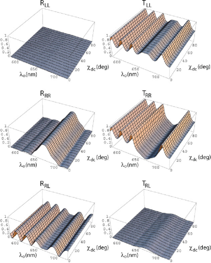
Figure 1: Reflectances and transmittances of a locally biaxial SCM slab of thickness $L=20\,\Omega$ as functions of the free–space wavelength $\lambda_{o}$ and the orientation angle $\chi_{dc}$ of the applied dc electric field, when $E^{dc}=10^{7}$ V m^-1 and $\theta=\phi=0^{\circ}$. The local crystallographic class of the SCM is orthorhombic $mm2$. Other parameters are: $\epsilon_{1}^{(0)}=4.72$, $\epsilon_{2}^{(0)}=5.20$, $\epsilon_{3}^{(0)}=5.43$, $r_{13}=34\times 10^{-12}$ m V^-1, $r_{23}=6\times 10^{-12}$ m V^-1, $r_{33}=63.4\times 10^{-12}$ m V^-1, $r_{42}=450\times 10^{-12}$ m V^-1, $r_{51}=120\times 10^{-12}$ m V^-1, all other $r_{JK}=0$, $h=1$, $\Omega=150$ nm, and $\chi=90^{\circ}$. As $T_{LR}=T_{RL}$ and $R_{LR}=R_{RL}$ to numerical accuracy, the plots of $T_{LR}$ and $T_{LR}$ are not shown.

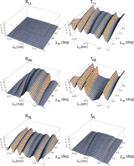
Figure 2: Same as Fig. 1, except that $E^{dc}=0.67\times 10^{9}$ V m^-1.

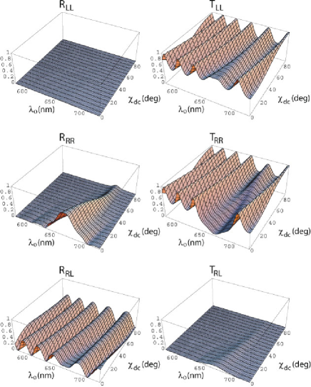
Figure 3: Same as Fig. 1, except that $E^{dc}=-0.67\times 10^{9}$ V m^-1.

Figure 4: Same as Fig. 1, except that $\chi=45^{\circ}$ and $E^{dc}=0.67\times 10^{9}$ V m^-1.

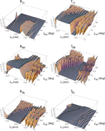
Figure 5: Same as Fig. 1, except that $\chi=45^{\circ}$ and $E^{dc}=-0.67\times 10^{9}$ V m^-1.

References

- [1] A. Lakhtakia, J.A. Reyes, Theory of electrically controlled exhibition of circular Bragg phenomenon by an obliquely excited structurally chiral material. http://www.arxiv.org/physics/0610073
- [2] R.W. Boyd, Nonlinear Optics, Academic Press, London, UK, 1992, Chap. 10.
- [3] A. Lakhtakia, R. Messier, Sculptured Thin Films: Nanoengineered Morphology and Optics, SPIE Press, Bellingham, WA, USA, 2005, Chap. 9.
- [4] J.A. Reyes, A. Lakhtakia, Electrically controlled optical bandgap in a structurally chiral material, Opt Commun. 259 (2006) 164–173.
- [5] J.A. Reyes, A. Lakhtakia, Electrically controlled reflection and transmission of obliquely incident light by structurally chiral materials, Opt. Commun. 266 (2006) 565–573.
- [6] M. Zgonik, R. Schlesser, I. Biaggio, E. Volt, J. Tscherry, P. Günter, Material constants of KNbO3 relevant for electro– and acousto–optics, J. Appl. Phys. 74 (1993) 1287–1297.
- [7] A. Lakhtakia, J. Xu, An essential difference between dielectric mirrors and chiral mirrors, Microw. Opt. Technol. Lett. 47 (2005) 63–64.
- [8] A. Lakhtakia, T.G. Mackay, Electrical control of the linear optical properties of particulate composite materials, Proc. R. Soc. Lond. A (2006) doi:10.1098/rspa.2006.1783