Universidad De Valencia
Departamento de Física Atómica, Molecular y Nuclear
Consejo Superior de Investigaciones Científicas
![[Uncaptioned image]](/html/physics/0611011/assets/x1.png)
![[Uncaptioned image]](/html/physics/0611011/assets/x2.png)
Depth of Interaction Enhanced
Gamma-Ray Imaging
for Medical Applications
To Judit and Eva
Abstract
A novel design for an inexpensive depth of interaction capable detector for gamma rays, suitable for nuclear medical applications, especially Positron Emission Tomography, has been developed, studied via simulations, and tested experimentally. The design takes advantage of the strong correlation between the width of the scintillation light distribution in continuous crystals and the depth of interaction of the gamma-ray. For measuring the distribution width, an inexpensive modification of the commonly used charge dividing circuits that allows analogue and instantaneous computation of the 2nd moment has been developed and is presented in this work. This measurement does not affect the determination of the centroids of the light distribution. The method has been tested with a detector made of a continuous LSO-scintillator of dimensions 42x42x10 and optically coupled to the compact large area position sensitive photomultiplier H8500 from Hamamatsu. The mean resolution in all non-trivial moments was found to be rather high (smaller than 5%). However the direct use of these moments as estimates for the three-dimensional photoconversion position turned out to be unsuitable. Especially, for gamma-ray impact positions near the edges and corners of the scintillation crystal, there is a strong interdependence between first and second moments. Nevertheless, it could be demonstrated that the measurement of the centroids is not affected at all by the simultaneous measurement of the second moment. Also it is has been shown that the bare moments can be used to reconstruct the true photoconversion position. This is a typical inverse problem also known as the truncated moment problem. Standard polynomial interpolation in higher dimensions has been adopted to reconstruct the impact positions of the gamma-rays from the measured moments. For this, a parameterization of the signal distribution has been derived in order to predict the moment response of the detector for all possible gamma-ray impact positions inside the scintillation crystal. The starting point is the inverse square law but other important effects have been included: refraction and Fresnel transition at the crystal-window interface, angular response of the photocathode, exponential attenuation of the scintillation light, and background from residual diffuse reflections at the black painted crystal surfaces. This model has been verified by experiment. For the three non-trivial moments, a very good agreement with measurements was observed. When using the reconstructed impact positions, the intrinsic mean spatial resolution of the detector was found to be for the transverse components and for the depth of interaction. Using directly the bare moments as position estimate, the intrinsic mean spatial resolution of the detector was found to be and , respectively. The cost for the required detector improvements are essentially negligible.
Resumen en Castellano
The pure and simple truth is rarely pure and never simple.
Antecedentes, Objetivos y Organización del Trabajo
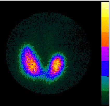
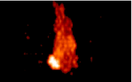
EN los últimos años, las técnicas de imagen en Medicina Nuclear han ganado en importancia debido a sus éxitos en el diagnóstico de oncología, neurología y cardiología. Imágenes tridimensionales pueden ser obtenidas actualmente por tomografía computerizada, mediante resonancia magnética nuclear (RMN) o mediante el empleo de isótopos radioactivos incorporados en una droga o en un compuesto biológico activo en general. La tomografía por emisión de positrones (Positron Emission Tomography o PET en inglés), gammagrafía y tomografía por emisión de un solo fotón (Single Photon Emision Tomography, SPECT) son las técnicas más usadas en diagnóstico por imagen en Medicina Nuclear y se basan en la reconstrucción de la distribución de pequeñas cantidades de radiofármacos administrados previamente. Si el radiofármaco administrado es específico para un cierto proceso metabólico, el empleo de los medios diagnósticos permite estudiar, caracterizar y valorar este mismo proceso. Las imágenes obtenidas son por tanto imágenes funcionales del cuerpo entero, de órganos o de las células. Por el contrario, imágenes médicas obtenidas por rayos X, tomografía computerizada, ecografía o similares aportan información morfológica y estructural del cuerpo o de los órganos. La RMN es capaz de proporcionar imágenes estructurales y funcionales, aunque la RMN funcional requiere la administración de grandes cantidades de sustancias de contrastes y su sensibilidad es de alrededor de seis ordenes de magnitud inferior que la de PET, SPECT y gammagrafía.
Los detectores de centelleo han constituido durante años los instrumentos primordiales para la detección de la radiación gamma procedente de los radiofármacos. Los más simples comprenden un único cristal de centelleo y un único fotodetector. Para obtener imágenes con dicho detector se inventó el escáner rectilíneo que aporta la información espacial al mover el detector sobre el objeto, registrando a la vez su señal junto con su posición actual. La primera cámara gamma fue desarrollada por Hal Anger en 1952 y consistió en un cristal y 7 fotomultiplicadores con una lógica analógica (lógica de Anger) que calcula las posiciones por suma con pesos. La configuración de cámaras gamma actuales se diferencia muy poco de este primer diseño aunque los constituyentes modernos de dichas cámaras se han mejorado significativamente en los últimos años. Hoy en día hay una amplia gama de cristales centelladores con muy diferentes propiedades y lo mismo ocurre con los fotodetectores. Una mejora muy importante de los últimos años es el uso de sistemas de dínodos especiales para que los fotomultiplicadores sean sensibles a la posición (Position Sensitive Photomultiplier Tube, PSPMT). Esto hizo posible el desarrollo de cámaras gamma muy compactas para su aplicación en la visualización de órganos pequeños. La gran mayoría de detectores de rayos- para todas las modalidades de Medicina Nuclear son cámaras de este tipo y que se han especializado para su función eligiendo los componentes más adecuados.
Desgraciadamente, los detectores de centelleo para rayos-, en general, padecen de un problema común. Dado que los cristales de centelleo han de ser de un grosor finito para conseguir parar los rayos- que se pretenden detectar, ellos mismos introducen una incertidumbre debido al hecho de que hasta el día de hoy existen pocas técnicas ya comercializadas para detectar la profundidad de interacción del rayo- dentro del cristal centellador. Como consecuencia, la posición del origen del rayo- no se calcula correctamente, conduciendo al error de paralaje. Este error es especialmente importante para la modalidad PET porque los fotones de aniquilación que se tienen que detectar tienen una energía alta de y en consecuencia su probabilidad de ser detectados es relativamente baja. Para detectores de PET con una eficiencia intrínseca aceptable, centelladores gruesos son necesarios. Debido a la falta de una componente de la posición de fotoconversión, el origen de la radiación no se puede computar exactamente siempre que la incidencia del rayo- no es normal respecto al plano del área sensible del fotodetector. Este error es especialmente importante para puntos de la región de interés lejos del centro del detector.
En los últimos años se han dedicado muchos esfuerzos a mejorar los parámetros claves como eficiencia intrínseca, resolución espacial y resolución energética. La detección de la profundidad de interacción es uno de estos campos de investigación. Entre los métodos más conocidos para determinar la profundidad de interacción figura la llamada técnica phoswich que usa el hecho de que los tiempos de desintegración (desexcitación) de diferentes centelladores se distinguen entre ellos y por lo tanto dan lugar a pulsos de luz de centelleo de diferente duración (Seidel et al. [Seidel:1999]). Usando dos materiales de centelleo diferentes, se puede determinar en cual de los dos cristales se ha efectuado la foto-conversión del rayo-. Las desventajas son la necesidad de dos cristales distintos para cada detector y la electrónica para diferenciar los dos tiempos de caída de la señal. Otra técnica muy usada es el light-sharing (Moses and Derenzo [Moses:1994]). Esta técnica se usa sobre todo con cristales pixelados y requiere dos fotodetectores de los cuales por lo menos uno ha de aportar la información espacial. Para cada pixel del centellador, se puede deducir la profundidad de interacción usando el reparto de la luz de centelleo entre los dos detectores. Uno de los fotodetectores tiene que ser un detector de semiconductores para no atenuar demasiado los rayos-. A parte de estas dos técnicas existen otras posibilidades no tan comunes. Una gran desventaja de los métodos mencionados es la necesidad de foto-detectores o/y cristales de centelleo adicionales para realizar la medida de la profundidad de interacción. Debido a que estos componentes son los más caros de un detector, estas técnicas encarecerían significativamente su construcción. Para permitir el amplio uso de métodos diagnósticos por imagen, tanto en medicina como en la investigación se requieren técnicas baratas y con razonables prestaciones. La segunda desventaja de todas las técnicas, a excepción del light-sharing, es que la resolución de la profundidad de interacción es no-continua (discreta) y que esta depende del tamaño de los pixels.
El objetivo principal de este trabajo fue el desarrollo de un detector de rayos- de un coste de fabricación reducido pero con prestaciones comparables a los de otros detectores actuales. Con este fin, se emplearon cristales de centelleo continuos y de grandes dimensiones, ya que de esta forma se puede evitar el costoso proceso de segmentación de los cristales. Se estima que este proceso encarece el cristal en un factor 7 debido al material del centellador que se pierde y también a las rupturas involuntarias. El uso de un fotomultiplicador sensible a la posición y con un área sensible elevada se fundamenta en una reducción en los costes de fabricación. Aunque estos dispositivos son relativamente caros, el precio por unidad de área sensible no es muy elevado. Varios estudios anteriores mostraron, que el empleo de cristales continuos es problemático especialmente para la tomografía por emisión de positrones. Debido a la elevada energía de los fotones de aniquilación, los cristales deben tener un grosor también elevado para asegurar una eficiencia intrínseca de detección suficientemente alta. Esto introduce variaciones importantes en la distribución de luz de centelleo que dependen de la profundidad del impacto de rayo- y de su posición en el plano del fotocátodo. Obviamente, la determinación de la posición del impacto es más difícil que en el caso de cristales pixelados en el que es suficiente identificar el pixel activo. El empleo de cristales continuos requiere analizar la distribución de luz y deducir a partir de este análisis los parámetros de impacto. Por su extremadamente bajo coste, el método más común es el algoritmo de centro de gravedad. Desgraciadamente, su uso junto con cristales gruesos produce efectos no lineales y dependientes de la profundidad de interacción cerca de los bordes de los cristales. Como resultado se perjudica la resolución espacial y energética en estas zonas, siempre que la profundidad de interacción no pueda ser medida (Freifelder et al. [Freifelder:1993], Siegel et al. [Siegel:1995], Seidel et al. [Seidel:1996], Joung et al. [Joung:2002]). No obstante, la configuración de un cristal continuo con un fotomultiplicador sensible a la posición y de área sensible amplia ofrece la estimación de la profundidad de interacción a partir de la anchura de la distribución de luz de centelleo detectada (Kenneth et al. [Kenneth:2001], Antich et al. [Antich:2002]). El principal problema consiste en medir esta anchura de forma rápida y con modificaciones de bajo coste. La digitalización de cada uno de los segmentos del ánodo permite su cálculo pero requiere muchos canales electrónicos. Si se implementara este método en un PET de animales pequeños compuesto por ocho módulos y cada uno con un PSPMT de 64 canales se requerirían en total 512 canales electrónicos. Para una versión con PSPMTs con 256 canales, el número se cuadruplica. Incluso con muy bajos costes por canal, el coste total para el sistema de adquisición de datos, almacenamiento y procesamiento sería elevado.
La idea fundamental para la resolución de este problema es una pequeña mejora de los circuitos de división de carga que se usan para la implementación analógica del algoritmo de centro de gravedad y se explica de la siguiente manera: el cómputo del centroide o del primer momento de una distribución discreta de cargas se puede realizar con una cadena de resistencias del mismo valor. Una carga que se inyecta en una de las interconexiones de la cadena se divide en dos fracciones. Según la posición donde se inyecta la carga, estas fracciones tienen diferentes valores siendo su suma siempre la misma. Si las fracciones de cargas varían linealmente con la posición, la diferencia de las cargas totales extraídas de los extremos de la cadena de resistencias es proporcional a la posición de la inyección, o, lo que es lo mismo, al centroide. La variación lineal de las cargas se consigue con una variación lineal de las resistencias y por lo tanto con resistencias de igual valor. Esto implica que la carga inyectada ve la conexión en paralelo de las dos ramas de la cadena. Como la variación de las resistencias con la posición es lineal, la variación de la impedancia total vista por la carga es cuadrática. Teniendo en cuenta que la anchura de la distribución de luz en cristales continuos esta correlacionada con la profundidad de interacción y que la desviación estándar es un buen estimador estadístico para la anchura de una distribución, la observación de la codificación cuadrática de los voltajes ofrece un método muy eficaz para la medida de la profundidad de interacción.
El punto de partida del presente trabajo se basó en estas observaciones ya que el desarrollo de circuitos de división de carga, con capacidad para medir un momento adicional sin perjudicar la medida de los centroides, puede proporcionar un diseño para detectores de rayos- relativamente barato pero con prestaciones similares a los de los diseños basados en cristales segmentados. No obstante, la mera medida del segundo momento o de la desviación estándar a partir del segundo momento y de los centroides no es suficiente para obtener una buena resolución espacial. Aunque la medida de la profundidad de interacción pueda ayudar a eliminar el error de paralaje, la resolución espacial intrínseca de los detectores empeora sustancialmente hacia los bordes del cristal debido a que los centroides están sometidos a una compresión no lineal y dependiente de la profundidad de interacción. Este último hecho posibilita la reconstrucción de la posición verdadera del impacto del rayo- a partir de los tres primeros momentos no triviales. Este problema es un problema inverso típico pero también se conoce como el problema de los momentos truncados (Tkachenko et al. [Tkachenko:1996]). Se trata de reconstruir la distribución a partir de una secuencia incompleta de los momentos de esta.
Este trabajo esta organizado de la siguiente manera. Tras una introducción general e histórica a la materia de Medicina Nuclear en el capitulo 1 se recapitulan en el capitulo 3 el diseño típico para detectores de rayos- para esta disciplina, sus limitaciones más comunes y propuestas de mejoras. El capitulo 2 resume la motivación para este trabajo. Una gran parte del trabajo se destinó al estudio de las distribuciones de luz de centelleo (capitulo 4) y al diseño y comportamiento teórico de circuitos de división de carga con capacidad de computar analógicamente el segundo momento (capitulo 5). Cada uno de los dos capítulos se puede leer con independencia. En los capítulos 7 y 8 se tratan respectivamente la validación experimental de los resultados de los capítulos anteriores y un algoritmo para reconstruir la posición del impacto del rayo- a partir de las medidas proporcionadas por las circuitos de división de carga modificadas. Finalmente, se resumen los resultados más importantes en las conclusiones (capitulo 9).
El capitulo 4 está dedicado al estudio del reparto de luz de centelleo sobre el área sensible del fotodetector. Para este fin se optó por el uso de una parametrización analítica de los efectos supuestamente más importantes. No se usó el método de las simulaciones Monte Carlo aunque es muy común para estudios similares. Las razones para esta decisión son la mejor comprensión de la distribución de luz de centelleo finalmente detectada y, una vez encontrado un modelo fiable y conforme con las observaciones, su adopción más sencilla a nuevos diseños de detectores. Para llegar a las mismas conclusiones que permite tal modelo analítico con simulaciones de Monte Carlo, muchas horas de simulación y muchas repeticiones con diferentes parámetros hubieran sido necesarias. En todo caso, simulaciones de Monte Carlo incluyen los mismos efectos físicos conocidos que se incluyeron en la parametrización usada en este trabajo pero con la ventaja de que el modelo analítico permite atribuir fácilmente detalles de la distribución a efectos fundamentales aislados. Por ejemplo, se puede estudiar muy bien con este modelo el efecto de usar cristales de extensión espacial finita. Simplemente hay que establecer un modelo para un cristal de dimensiones finitas y otro con dimensiones infinitas y comparar los resultados. En el caso de simulaciones de Monte Carlo, ni siquiera es posible hacer esta comparación. A parte de esto, las simulaciones se llevan a cabo evento por evento, es decir, fotón por fotón, y por lo tanto requieren un tiempo elevado de computación.
En el modelo de la distribución de luz de centelleo se incluyeron lo siguientes efectos: El punto de partida fue la ley del inverso cuadrado que describe el reparto de intensidades en superficies esféricas para fenómenos de radiación. Se ha de tener en cuenta que los fotodetectores en general (y en particular el que se usa para este trabajo) disponen de una superficie plana para la detección de los fotones. Por lo tanto hay que multiplicar por el coseno del ángulo de incidencia para compensar la diferencia de las áreas irradiadas. Otro efecto fundamental es la auto-absorción de luz de centelleo por el mismo cristal centellador. Aunque esta es normalmente muy baja por razones obvias, puede resultar relevante para posibles caminos de luz muy largos. La auto-absorción obedece la ley de atenuación exponencial. Sobre todo para puntos de observación lejos de la posición de impacto se reducirá la intensidad detectada de la luz. Estrictamente, la atenuación exponencial incluye dos efectos: la absorción y la dispersión elástica de la luz incidente. Esta última contribución causa un fondo de luz ya que la luz distribuida puede ser detectada en otro punto de la superficie sensible del fotodetector. Se supone que esta contribución es muy baja y no se incluyó en el modelo.
El siguiente efecto es debido al interfaz óptico entre el fotodetector y el cristal de centelleo. Para su protección, los fotodetectores disponen siempre de una ventana de entrada hecha de un material transparente para la radiación que se quiere detectar. Esta ventana es de un grosor finito y en general su índice de refracción es diferente al del cristal de centelleo. Muchos de los cristales de centelleo con aplicación para Medicina Nuclear tienen un índice de refracción muy elevado y mayor al de la ventana de entrada del fotodetector. En este interfaz óptico se produce reflexión total cuando el ángulo de incidencia supera al ángulo crítico. Debido a este hecho, el cristal centellador ha de acoplarse al fotodetector mediante grasa óptica de un índice de refracción intermedio. De otro modo no se pueden evitar la inclusión de una fina capa de aire que reduce considerablemente la eficacia de recolección de luz. La luz de centelleo que pasa a la ventana de entrada se desvía según la ley de Snell y la amplitud de la misma viene descrita por las ecuaciones de Fresnel que también reproducen bien la reflexión de una fracción residual de la luz incidente para ángulos de incidencia menor al ángulo crítico. La refracción de Snell y la transmisión y reflexión de Fresnel se incluyeron en el modelo analítico suponiendo además, que la luz de centelleo no esta polarizada. El siguiente fenómeno que se tuvo en cuenta requiere especificar que tipo de fotodetector se usa para el diseño del detector de rayos-, ya que las propiedades de los mismos pueden resultar muy diferentes. Como ya se había mencionado arriba, para el presente trabajo se optó por un fotomultiplicador sensible a posición. La sensibilidad del fotocátodo del mismo no es constante para diferentes ángulos de incidencia. Esto es debido a varias circunstancias. Una de ellas es la limitación de que los fotocátodos tienen que tener un grosor muy pequeño para asegurar que los fotoelectrones puedan salir del mismo y ser recolectados por el primer dínodo. Por esta razón, la eficiencia cuántica no es muy elevada porque una fracción alta de la luz de centelleo es transmitida sin ser detectada. Los fotones de luz con un ángulo de incidencia elevado tienen que recorrer una trayectoria más larga dentro del fotocátodo y su probabilidad de crear un fotoelectron es más elevado.
Aparte de la luz de centelleo que llega directamente a ser detectada por el fotomultiplicador también existen contribuciones debidas a reflexiones en los cinco lados del cristal centellador que no están acopladas ópticamente al fotodetector. Se conocen numerosos estudios que demuestran que el acabado de estas superficies es muy importante para la eficiencia de recolección de luz y la resolución espacial. No obstante, el método de deducir la profundidad de interacción a partir de la anchura no permite usar acabados reflectantes sino que requiere la supresión de esta luz. Por este motivo se cubrieron estos lados con resina epóxica negra. Aunque el coeficiente de reflexión de este material es muy bajo, el área total de las superficies cubiertas con este material es elevado, y, como se verá en el capitulo 7 de los resultados experimentales, no es despreciable especialmente para profundidades de interacción cerca del limite superior de los posibles valores. Ya que los cristales de centelleo no están pulidos sino cubiertos con resina epóxica negra, dicha reflexión residual es supuestamente difusa y su comportamiento se aproximó con la ley de Lambert. También hay que tener en cuenta que gran parte de la luz procedente del punto de fotoconversión no es capaz de entrar a la ventana de entrada debido a la reflexión total. En su lugar, esta luz reflectada se refleja una segunda vez y de forma difusa en las otras superficies negras. Esta contribución es igual de importante que la luz que se refleja directamente en las superficies negras y por lo tanto se incluyó en el modelo analítico. Otros efectos como refracción, transmisión de Fresnel o sensibilidad angular del fotocátodo no se tuvieron en cuenta para la luz de fondo debido a la reflexión difusa. La distribución de señal observada en los segmentos del ánodo del fotodetector es el resultado de la acción conjunta de todos los efectos descritos y suponiendo como procesos ideales la recolección de los fotoelectrones por el sistema de dínodos y su multiplicación.
En el siguiente capítulo 5 se analizaron detalladamente las propiedades de diferentes implementaciones de circuitos de división de carga. También se mostró como se pueden mejorar estos circuitos para que computen simultáneamente el segundo momento sin perjudicar a los centroides. Aparte de la lógica de Anger tradicional existen otras posibilidades de implementación del algoritmo de centro de gravedad con redes de resistencias (Siegel et al. [Siegel:1996]). Las tres variantes más comunes muestran una calidad de posicionamiento muy parecido pero hay importantes diferencias en la cantidad de resistencias necesarias. Como se ha explicado anteriormente, las corrientes (o equivalentemente las cargas) inyectadas causan un potencial codificado cuadráticamente. Esto se debe a la codificación lineal para la computación de los primeros momentos, los llamados centroides. Por lo tanto un sumador analógico ya es suficiente para obtener una única señal adicional que representa el segundo momento. Ya que los componentes necesarios para este sumador son un amplificador operacional y unas pocas resistencias y condensadores, el coste total viene únicamente dado por el canal electrónico adicional (por detector de rayos-) para la digitalización del segundo momento. Si retomamos el ejemplo de un PET para animales pequeños construido con 8 detectores con cristales continuos, el uso del algoritmo de centro de gravedad analógico reduce el numero total de canales electrónicos necesarios a 32 en vez de 512 para PSPMTs de 64 ánodos o de 2048 para PSPMTs de 256 canales. Además el número de canales electrónicos necesarios no depende del numero de segmentos de ánodos del tipo de PSPMT usado. Esto hace el método del centroide muy versátil. Con la mejora para la medición simultánea de los segundos momentos harán falta 40 canales en vez de 32 lo que no supone ningún problema de realización.
Aunque el comportamiento de las diferentes variantes de los circuitos de división de carga es muy similar para el centroide, el comportamiento respecto a la medida del segundo momento muestra importantes diferencias. Un aspecto es la simetría en el comportamiento de los circuitos de división de cargas respecto al intercambio de las coordenadas espaciales e . La lógica de Anger original posee esta simetría inherentemente. Sin embargo, tanto las configuraciones electrónicas de la versión basada en cadenas proporcionales de resistencias como la de la versión híbrida, que es una mezcla de las otras dos, rompen esta simetría. Para restablecer la simetría por completo para los centroides en los dos casos, algunas resistencias tienen que tener valores determinados que dependen de la configuración y los valores de las otras. En el caso del segundo momento se puede restablecer la simetría sólo para la variante híbrida. Para la versión basada en cadenas proporcionales de resistencia no es posible fijar los valores de las resistencias de una manera tal que el circuito se comporte exactamente igual en la medida de los cuatro momentos (energía, centroides y segundo momento) para las dos direcciones espaciales. No obstante, en el caso optimizado, la disimetría residual para el segundo momento es menor del 1 % y los otros tres momentos se comportan de forma totalmente simétrica. Para obtener esta simetría óptima hay que aceptar que el segundo momento contiene contribuciones de los ordenes , y . Este hecho tiene consecuencias cuando se quiera usar la desviación estándar como estimador de la profundidad de interacción pero no significa ninguna desventaja para el método de reconstrucción de la posición que se presentara en el capitulo 8.
Otro aspecto estudiado en el capitulo 5 es la influencia de la impedancia de entrada del sumador analógico sobre la medida de los centroides. Obviamente no se puede permitir que la medida complementaria reduzca significativamente la calidad de las medidas de los centroides o la de la energía. Para que este requisito se cumpla hay que asegurar que el sumador extraiga muy poca corriente de los circuitos originales. Desgraciadamente no se pueden usar seguidores de tensión para este fin ya que el consumo medio de tal amplificador sería de unos que asciende a unos para el modulo entero si el PSPMT tiene 64 segmentos de ánodo. La impedancia de entrada de una rama del sumador analógico viene dada aproximadamente por la resistencia de entrada que a su vez determina el peso con que la señal correspondiente entra en la suma total. Por lo tanto, estas resistencias tienen que tener valores elevados pero no deben superar cierto límite, ya que valores demasiado altos introducirán ruido térmico. Como criterio de diseño se usa el hecho de que las resistencias reales y comerciales tienen una tolerancia en su valor de 1 %. Carece de sentido calcular los valores de resistencia con mayor precisión. Este aspecto se tiene que tener en cuenta para las tres variantes de los circuitos de división de carga.
El efecto de dispersión de Compton de los rayos- dentro del cristal centellador es el objetivo del capitulo 6. El modelo de la distribución de señal que se desarrolló en el capitulo 4 es solo válido para eventos que depositan toda su energía en una sola interacción, es decir, para fotoconversiones por efecto fotoeléctrico. Especialmente para los fotones de energía de la modalidad de PET cabe la posibilidad de que experimenten varias dispersiones de Compton antes de ser absorbidos por completo. Obviamente, sólo la posición de la primera interacción corresponde a la linea de vuelo correcta del fotón gamma. Con la lógica de Anger y sus variantes descritas anteriormente no es posible determinar esta posición. En su lugar, se medirá el centroide de la superposición de varias distribuciones procedentes de deposiciones puntuales de energía, ya que cada interaccíon por efecto Compton depositará una fracción de la energía inicial del fotón incidente. Esto resultará en un error de la posición de impacto medida y del segundo momento y reducirá la resolución espacial transversal y la de la profundidad. Para estimar el impacto de dispersión de Compton sobre dicha resolución se llevó a cabo una simulación de Monte Carlo con el paquete GEANT 3 (Brun and Carminati [Geant3:1994]). Se simularon las interacciones de 20000 rayos- de en un cristal centellador de LSO con dimensiones . Como resultado se pueden resumir las siguientes dos observaciones. La incertidumbre introducida por este efecto es en la mitad de los casos menor a tanto para las coordenadas paralelas al fotocátodo como para la componente normal. La otra mitad de los eventos se reparte en una cola muy larga de baja intensidad atribuyendo sobre todo ruido de fondo por que las distancias son más grandes que las resoluciones espaciales medidas obtenidos en los capítulos 7 y 8. El otro efecto observado es la opresión de eventos de dispersión hacia delante, o sea con ángulos de dispersión cerca de cero grados. Esta opresión se puede explicar de la siguiente manera. Debido a la formula de Klein-Nishina (Leo [Leo:1994]), la dispersión de Compton para rayos- de favorece fuertemente ángulos de dispersión alrededor de cero grados. Además, para esta energía, la probabilidad de que un fotón experimente una interacción de Compton es ya muy reducida y se requiere un grosor elevado para parar eficientemente dichos rayos-. No obstante, el cristal simulado es solo de un grosor de y un gran número de fotones pasará el cristal sin ser detectado. Otro número elevado de fotones experimentará una interacción de Compton con un ángulo de dispersión muy pequeño. En consecuencia, la energía del fotón que sale seguirá siendo muy elevada y la probabilidad de interacción muy baja. Por lo tanto, todos estos fotones probablemente escapen del cristal sin ser detectados. Sin embargo, en el caso de que la primera interacción sea de tipo Compton y con un ángulo de dispersión elevado, la pérdida de energía del fotón también será elevada y el fotón que salga de esta interacción tendrá una probabilidad de interacción mucho más alta. Aparte de esto se moverá más o menos en paralelo al fotocátodo de forma que aumentará aún más la probabilidad de su detección, ya que la extensión transversal del cristal simulado es el doble de la extensión normal. Estos efectos dan lugar a una predisposición hacia ángulos de dispersión elevados para el subconjunto de eventos detectados. Probablemente esta es la causa de que el método para medir la profundidad de interacción que se presenta en este trabajo de lugar a resultados suficientemente buenos para su aplicación en detectores reales.
El siguiente capítulo 7 abarca las verificaciones experimentales de los resultados de los tres anteriores capítulos. Para llevar a cabo los experimentos se usaron dos detectores iguales. Cada uno esta compuesto por un único cristal del centellador LSO de grandes dimensiones () y de un PSPMT del tipo H8500 de la empresa Hamamatsu Photonics Inc. (Hamamatsu [data:H8500]). Debido a la radiactividad intrínseca del LSO, medidas con fuentes de actividad menor de se tienen que llevar a cabo en coincidencia temporal (Huber et al. [Huber:2002]). A parte de ello, medidas en coincidencia con dos detectores de rayos- con resolución espacial permite una colimación electrónica del haz. El fotomultiplicador H8500 tiene un área sensible de y dispone de 64 segmentos de ánodo. La señal de disparo para el módulo se derivó de los últimos dínodos de los PSPMT. Un discriminador del tipo leading edge admitió solo eventos a partir de cierto umbral y creó pulsos lógicos de anchura temporal de . A partir de estas dos señales se creó la señal de coincidencia temporal con una puerta lógica de función booleana AND que sirvió para dos funciones. Se usó para derivar otro pulso lógico de anchura temporal de y retrasado por . El flanco de subida de este pulso se usó para iniciar el proceso de integración y su flanco de bajada la finalizó. El resultado de esta integración de la corriente es proporcional a la carga total extraída de los fotomultiplicadores y fue convertida a valor digital. Las operaciones de restauración de línea base, integración de carga y digitalización se realizaron con una tarjeta de 12 canales electrónicos (Zavarzin and Earle [Zavarzin:1999]). La ventana temporal se obtiene como suma directa de las dos anchuras de las señales que proporcionan los discriminadores. Estos se ajustaron a su límite inferior de con lo cual la ventana de coincidencia fue de unos .
Una vez digitalizadas las 10 señales de los dos módulos se transfirieron al ordenador para la computación de los 4 momentos. Un modulo se usó como detector de testeo mientras el otro sólo tuvo las funciones de detector de coincidencia temporal y de la colimación electrónica. La distancia total entre los dos módulos era de unos y la fuente radiactiva (, actividad nominal ) se colocó entre ellos de forma centrada y muy cerca (a unos del cristal) del detector de testeo. De esa manera se pudo colimar el haz electrónicamente al seleccionar eventos de coincidencia temporal con una posición de impacto (en el detector de coincidencia) que cayó dentro de un circulo central de diámetro . Por argumentos geométricos, la región de posiciones en el detector de testeo tiene que ser un circulo de diámetro . Mientras el detector de coincidencia y la fuente radiactiva estuvieron alineados y estacionarios, el detector de testeo estuvo montado encima de una mesa - computerizada. Esto permitió variar la posición del impacto del rayo- a lo largo del plano del fotocátodo y se pudieron medir de forma automática los diferentes momentos en diferentes posiciones.
Dos detalles muy importantes que hay que tener en cuenta son los siguientes. Primero, la fuente de radiación no fue puntual sino que tuvo un diámetro de aproximadamente . Además, como el decae pro radiación , estos positrones penetran hasta dentro la cápsula de resina. Por lo tanto, el diámetro efectivo que se obtiene a partir de la radiación de aniquilación es diferente a . Se estimó por simulaciones Monte Carlo, que el diámetro efectivo es de unos . La resolución espacial que se espera para el detector de rayos- diseñado en este trabajo es del mismo orden y por lo tanto se tuvo que corregir mediante el diámetro efectivo de la fuente radiactiva. El segundo efecto que juega un papel muy importante es que no se puede prepara el haz de fotones gamma para que estos interaccionen en una profundidad del cristal determinada. Mientras las componentes paralelas al plano del fotocátodo se puede prepara fácilmente posicionando el detector de testeo en la posición deseada, la profundidad de interacción es una variable completamente aleatoria. Sin embargo, diferentes detecciones con diferentes profundidades causan distribuciones de luz de centelleo con diferentes segundos momentos y por lo tanto se pueden distinguir estos sucesos si la resolución en la medida de este momento es suficientemente alta. Se ha de observar una estadística muy característica para este momento que refleja una caída exponencial debido a la absorción de los rayos- dentro del cristal de LSO, una resolución intrínseca para el segundo momento y los limites superiores e inferiores para el momento, ya que el cristal es de un grosor finito y solo se pueden detectar eventos cuyo segundo momento corresponda a una profundidad real existente y de acuerdo con las dimensiones del cristal. Se ha ideado un modelo que describe bien el comportamiento de dicha distribución y que permite extraer los parámetros clave que son los limites superiores e inferiores y la resolución intrínseca.
Una vez acabados todos estos preparativos se verificó el modelo de la distribución de luz establecido en el capitulo 7. Para este fin se midieron los cuatro momentos en posiciones distribuidas de forma centrada, cartesiana y con una distancia de entre ellas. Estas medidas se compararon con las predicciones del modelo analítico para las mismas posiciones y momentos. Para finalizar este capitulo, se estimó la resolución en la posición tridimensional del detector propuesto en el caso de que se usaran estos mismos momentos como estimador de posición de impacto y energía. Para obtener resoluciones reales se hubo que corregir por la compresión que introducen los centroides y por el efecto del diámetro efectivo de la fuente radiactiva.
El capítulo 8 se motivó por las observaciones en los capítulos 5 y 7. Los resultados del capitulo 7 muestrearon, que los momentos de la distribución de luz se pueden medir con buena resolución aunque estos momentos no constituyen estimadores de gran validez para la posición de impacto real. También se observó en el capitulo anterior, que el modelo analítico para la distribución de señal derivada en el capitulo 4 proporciona momentos que concuerdan muy bien con las medidas. Por lo tanto se tiene un modelo que es capaz de predecir muy bien el comportamiento de las señales que proporciona el detector de rayos-. A parte de esto se tiene para cada posición tridimensional de impacto y su energía un número total de cuatro momentos de la distribución. La reconstrucción de la posición real a partir de estos momentos es un típico problema inverso y su viabilidad se estudió en el capitulo 8. El problema también se conoce como problema de momentos truncados que se ha estudiado intensivamente desde su descubrimiento (Talenti [Talenti:1987], Kreĭn and Nudel’man [Krein], Jones and Opsahl [Jones:1986]). Desgraciadamente, todos los algoritmos basados en este método requieren una secuencia de más de 4 momentos para una reconstrucción viable. Por lo tanto se optó por la interpolación polinómica que se aplicó con éxito para un problema muy similar (Olcott et al. [Olcott:2005]). Este método usa para la reconstrucción de las posiciones reales una matriz de corrección que se obtiene a partir de la inversa de Moore-Penrose de los coeficientes de los polinomios de interpolación de los momentos y sus correspondientes posiciones de impacto. El funcionamiento correcto de este método se comprobó usando los datos de medida en todas las 81 posiciones obtenido en el capitulo 7 de forma cualitativa. Después se midió la resolución espacial del propuesto detector en los 81 puntos usando esta vez la posición reconstruida en vez de los momentos y se compararon con los anteriores resultados usando los momentos como estimadores de posición. Se intentó también, pero sin éxito, la reconstrucción de la energía verdadera. Otra vez hubo que corregir por el efecto del diámetro efectivo de la fuente radiactiva y el de la compresión residual de las posiciones reconstruidas.
Para terminar el trabajo se resumieron en capitulo 9 las principales conclusiones de los diferentes capítulos y algunas perspectivas para investigaciones futuras. Por último se incluyeron los apéndices A-D que contienen algunos datos de interés como radiofármacos comunes, centelladores típicos, resultados complementarios y configuraciones electrónicas detalladas.
Discusión de los resultados y conclusiones
En el presente trabajo se ha desarrollado un método innovador para medir la profundidad de interacción de rayos- en cristales de centelleo gruesos y continuos. La nueva técnica consiste en estimar este parámetro usando la anchura de la distribución de luz de centelleo en los cristales que es detectada por un fotomultiplicador. Para su medida rápida y sencilla se ideó una modificación de muy bajo coste de los circuitos convencionales de división de carga que se usan con gran frecuencia para la determinación de la posición del impacto en detectores de rayos- para la Medicina Nuclear.
Para que la calidad de la imagen médica sea alta respecto a la relación señal a ruido, el contraste y la resolución espacial, el detector de rayos- tiene que proporcionar información sobre la posición tridimensional del impacto, especialmente para al modalidad de PET. Sin esta información, se introduce un error de paralaje para todas las posiciones fuera del centro y que tiene mayor importancia en zonas de la región de interés que están lejos de este centro. Es más, detectores de rayos- de tipo Anger convencionales aproximan los componentes transversales de la posición de impacto usando los centroides, o bien los primeros momentos normalizados, de la distribución de señal. Varios grupos han observado que el algoritmo de centro de gravedad como estimador de posición de impacto produce errores no-lineales y dependiente de la profundidad de interacción para cristales gruesos. Esto perjudica la resolución espacial cerca de los lados y especialmente en las esquinas del detector.
En el capitulo7 se discutieron con detalle los errores debidos al algoritmo de gravedad. Se reveló que la compresión de las posiciones es causada por la ruptura de la simetría de la distribución de señal por culpa de un cristal de dimensiones espaciales finitas. Por esta razón, la insuficiente resolución espacial obtenida con cámaras Anger convencionales no es debida a una medida de baja resolución de los momentos por los circuitos de división de carga, sino a que la aproximación de la posición de impacto por estos momentos no es valida para estas regiones del área sensitiva. No obstante, se mostró en el capítulo 7 que los momentos pueden ser medidos con alta resolución. Igualmente se observó, que la impedancia de entrada de los circuitos de división de carga están codificados cuadráticamente con la posición y por tanto producen voltajes con la misma propiedad bajo la inyección de corrientes procedentes de los fotomultiplicadores. Una configuración tan simple como un sumador analógico puede ser usado para sumar estos voltajes y proporcionar una señal adicional linealmente correlacionada con el segundo momento. Junto con la observación de otros grupos (Rogers et al. [Rogers:1986], Kenneth et al. [Kenneth:2001], Antich et al. [Antich:2002]) de que la anchura de la distribución depende fuertemente de la profundidad de interacción, esto proporciona un método potente para medir la misma profundidad de interacción.
En el capítulo 5 se demostró, que todas las versiones conocidas de circuitos de división de carga pueden ser modificados con un sumador analógico para medir el segundo momento. También se vio, que las diferencias teóricas en las cualidades de estas versiones solo varían poco de una a otra. Esto se observó también experimentalmente para los centroides y la carga total (Siegel et al. [Siegel:1996]) y por lo tanto el criterio para la elección de la variante del circuito de división de carga puede ser la complejidad de la red de resistencias. Se dieron también en el capítulo 5 expresiones explicitas para la dependencia de los voltajes y la suma de ellos en función de la posición de la corriente inyectada y en función de la configuración del circuito. Comparaciones con simulaciones con Spice, (Simulation Program with Integrated Circuits Emphasis, Tietze and Schenk [Tietze]) concuerdan muy bien con las predicciones hechas con estas fórmulas y las diferencias máxima es en todos los casos menor de un 3 %. Un resultado complementario está relacionado con el comportamiento de la simetría de los circuitos. La lógica de Anger convencional es inherentemente simétrica respecto al intercambio de las posiciones e , pero las otras dos versiones no lo son. Afortunadamente se puede restaurar esta simetría por completo para los centroides, y, en el caso de la red híbrida, también para el segundo momento. Para el circuito basado completamente en cadenas de resistencias, sólo se puede minimizar la disimetría, aunque se consiguen valores residuales muy pequeños de 1 % o menos. Para conseguir esto, hay que aceptar que se introducirán ordenes de , y en el segundo momento. Esto sólo supone un problema si se quiere usar la desviación estándar como estimador para la profundidad de interacción. Para el método presentado en el capítulo 8, estos ordenes elevados no suponen ninguna complicación adicional. La impedancia de entrada de los sumadores se tiene que dimensionar de tal forma, que evite la extracción excesiva de corriente del circuito para los centroides. En caso adverso, esto perjudicaría a los mismos lo que no es aceptable. La solución ideal sería usar seguidores de tensión, ya que estos tienen una impedancia de entrada muy elevada. Su uso no es posible debido a su alto consumo. Esta opción esta reservada para un futuro diseño de un circuito ASICs (Application-Specific Integrated Circuit) y no forma parte del presente trabajo. Por estas razones, los valores de las resistencias para los sumadores tienen que ser en general muy elevados. Una indicación adversa al uso de valores demasiado altos es el ruido térmico. En el presente caso se obtuvieron resultados aceptables con valores de resistencias al sumador que extraen como máximo un 1 % de corriente en cada nodo del circuito de división. Para la realización del detector de rayos- se usó un circuito basado completamente en cadenas de resistencias y un sumador con 64 entradas ya que esta versión es la que más fácilmente se implementa.
En el capítulo 7 se presentaron medidas de los 4 momentos de un detector real. El detector está basado en un cristal de LSO de dimensiones de y un fotomultiplicador H8500. Los experimentos muestran que los centroides no están afectados por la medida del momento adicional. La resolución media en estos momentos es menor del . También se observó, que la aproximación de usar estos cuatro momentos como posición de impacto es inadecuada. Los mismos resultados obtuvieron otros grupos que investigaban el comportamiento de los centroides sin medida del segundo momento. El momento trivial representa la energía del impacto y los momentos no-triviales son los centroides y el segundo momento. El momento trivial se ve afectado por efectos y condiciones adicionales y no alcanza la resolución de los momentos no triviales. Una causa para esto es la inhomogeneidad del fotocátodo de los fotomultiplicadores. La eficiencia y la ganancia puede variar de un segmento de ánodo a otro hasta alcanzar diferencias de un factor 3. Esta falta de uniformidad introduce una variación de energía detectada adicional e importante. Por otro lado, el método para medir el segundo momento que se presenta con este trabajo requiere que todas las superficies que no están acopladas al fotodetector estén cubiertas de una capa muy absorbente para evitar reflexiones, ya que estas destruyen por completo la correlación de la profundidad de interacción con el segundo momento. Obviamente esto reduce la eficacia de recolección de luz y por lo tanto la resolución energética. Este efecto es de muy elevada importancia en las esquinas del detector y las resoluciones energéticas son muy bajas en estas zonas. En los experimentos se observó una resolución energética media del con el valor mínimo en el centro del y el valor máximo () en una de las esquinas. La degradación de la resolución energética se compone de dos efectos. Un efecto importante es la variación del total de la luz detectada por razones geométricas. Para puntos de fotoconversión muy cerca de una superficie negra, menos luz es detectada y el máximo del espectro está en canales más bajos. En los histogramas de energía se superponen muchos eventos con diferentes posiciones y por lo tanto se obtiene una única distribución muy ancha debido al movimiento del máximo del fotopico. Este efecto se puede corregir una vez obtenida la posición real del impacto y conociendo el comportamiento del momento trivial para todo el volumen del cristal. El hecho de que no se podía corregir la energía como parte del presente trabajo es probablemente debido a una resolución espacial aún no suficiente para este fin. El otro efecto es el de la variación por estadística de Poisson. Este efecto no se puede corregir con la posición aún teniendo una resolución muy buena en la misma. El uso de retroreflectores (Karp and Muehllehner [Karp:1985], Rogers et al. [Rogers:1986], McElroy et al. [McElroy:2002]) puede probablemente mejorar este aspecto.
El modelo para la distribución de luz se verificó experimentalmente en el capítulo 7. Para los tres momentos no triviales se observó que las predicciones del modelo reproducen muy bien las medidas de estos momentos. Las desviaciones siempre estaban por debajo del , excepto para el momento trivial. En este último caso, el modelo no reproduce correctamente todos los detalles de las medidas. Las predicciones del modelo concuerdan bien con los momentos medidos para profundidades de interacción cerca del limite inferior. En el caso opuesto, es decir, para profundidades de interacción cerca del limite superior, se producen discrepancias obvias entre el modelo y las medidas. Estas observaciones se pueden explicar fácilmente con las aproximaciones que se hicieron para llegar al modelo para la distribución de luz de fondo. Se suponía que la contribución total no fuera muy elevada. No obstante, para profundidades de interacción elevadas, la contribución de luz de fondo a la distribución total se vuelve muy importante. Esto se verificó con un modelo alternativo que no disponía de luz de fondo. Sin luz de fondo, el modelo reproduce las variaciones del momento trivial a lo largo del fotocátodo mucho peor. Sin embargo, los resultados para los momentos no-triviales se reprodujeron con una calidad muy similar. Esto se espera, ya que la normalización de estos momentos elimina de forma eficiente la dependencia del momento trivial. Razones para los errores en estos momentos son probablemente la influencia de dispersión de Compton y sobre todo la precisión mecánica. Aunque la mesa - dispone de muy buena precisión, el resto del montaje, que incluye la fijación de la fuente y de las carcasas de los detectores de rayos-, no alcanza la misma precisión. Esta última fuente de error ha de minimizarse para obtener mejores resultados en medidas futuras.
El capítulo 8 se dedicó a encontrar un algoritmo para la reconstrucción de la posición de impacto real a partir de los momentos. Para este fin se usó el modelo de la distribución de señal, ya que en el capítulo 7 se verificó que esta reproduce bien los momentos no-triviales. Se usó el modelo para predecir el comportamiento del detector en 40000 diferentes posiciones de impacto. La respuesta del detector consiste en los tres momentos no-triviales y el momento trivial. Los resultados para los dos centroides y el segundo momento se interpolaron con ordenes 12 para los componentes transversales y con orden 5 para el componente normal. Según el capítulo 8, se puede usar la inversa de Moore-Penrose en conjunto con las 40000 posiciones de impacto para obtener una matriz del detector que permite la reconstrucción de la posición de impacto. A continuación, se calcularon las posiciones a partir de los momentos. La resolución espacial del detector era en este caso de para las dos dimensiones transversales y de para la profundidad de interacción. Esto presenta una mejora sustancial con respecto a la resolución del detector obtenido usando los momentos ( y ) para las mismas coordenadas. Especialmente el resultado para la resolución en profundidad es muy importante, ya que existen muy pocos métodos que llegan a esta resolución. No se consiguió corregir por completo la no-linealidad de la posición con este método. Con los valores mencionados aquí, se obtuvo una no-linealidad residual de aproximadamente el . Este error es del mismo orden que el error del modelo observado en capítulo 7. Probablemente, la precisión del modelo analítico tiene que superar este valor para obtener mejores linealidades y resoluciones. La resolución espacial y tridimensional que se obtiene de momento con el método presentado no es suficiente para reconstruir la energía real a partir del momento trivial con la información de los momentos no-lineales.
En este trabajo se ha presentado un método simple y barato para medir el segundo momento de la distribución. Se ha mostrado, que esta información adicional se puede utilizar conjuntamente con los centroides para reconstruir la posición real del impacto. De esta manera se pueden realizar detectores de rayos- para Medicina Nuclear que proporcionan información sobre la profundidad de interacción y que permiten reducir el error de paralaje. El método presentado es apto para cualquiera de las modalidades en las que hace falta saber la información de profundidad y es muy barato. No obstante, el algoritmo de inversión no es óptimo y requiere futura investigación.
Contents
toc
Chapter 1 Historical Introduction
Fortune knocks but once, but misfortune has much more patience.
GAMMA-ray imaging covers only a small area of the large spectrum of imaging techniques applied to medical diagnostics. Many of these techniques, e.g. Radiography, Sonography and Nuclear Magnetic Resonance (NMR), have already been in routine use for many years. Others are at an early stage of development and far from being widely applied. Since 1895, when the possibility of using X-rays for planar transmission imaging was discovered by Wilhelm Conrad Röntgen at the university of Würzburg (Germany), all techniques have been under active development to a greater or lesser extent. In that year, Röntgen observed a green colored fluorescent light generated by a material located a few feet away from a working cathode-ray tube. He attributed this effect to a new type of ray that he supposed had been emitted from the tube and found that the penetrating power of the new ray also depended on properties of the exposed substances casting the object’s density distribution into a two dimensional projection. One of Röntgen’s first experiments with the newly discovered radiation was a projection image of the hand of his wife Bertha. An important contribution to radiography diagnostics was made by Carl Schleussner. He developed the first silver bromide photographic X-ray films, which made archival storage of diagnostic results possible and also lowered the necessary exposure. Within only a month after the announcement of the discovery, several medical radiographs had been built. They were used by surgeons to guide them in their work and only a few months later they were used to locate bullets in wounded soldiers.
Although radiography was the first medical imaging modality, the first attempts to see inside the human body without invasive operation go back a longer time (Wayand, [Wayand:2004]). When in the year 1879 Maximilian Nitze and Josef Leiter introduced the first optical system in Vienna using a platinum glow wire as light source, they laid the foundations of Endoscopy. Only two years later and also in Vienna, the surgeon Jan Mikulicz-Redecki demonstrated the first Gastroscopy (telescopic inspection of the inside of the gullet, stomach and duodenum). However, the first commercial semi-flexible Gastroscope, designed by Georg Wolf and Rudolph Schindler, did not appear until 1932.
Thermography and Electrocardiography are two other examples of medical imaging modalities that were known before the discovery of X-rays by W.C. Röntgen. As for thermography, the knowledge even goes back to Hippocrates, who first obtained thermograms of the chest. He proposed covering the patient’s thorax with a piece of thin linen soaked with earth, and observing the process of drying. At the warmer areas of the thorax, the earth-soaked cloth dries faster and the pattern of enlargement of the dry areas represents the temperature distribution (Otsuka et al. [Otsuka:1997]). Sir John Herschel rediscovered thermography in 1840 and created the first thermal image of modern times by evaporating a thin film of alcohol applied to a carbon-coated surface. The first detector that was able to measure infrared radiation was invented in 1880 by Samuel P. Langley, 80 years after the discovery of this radiation by Sir William Herschel. Herschel measured the temperature of light split by a prism and found that the temperature increased through the colors of the spectrum and furthermore continued to increase into the non-visible region, today called infrared. Also, bio-electricity was known long before the late 19th century. It was first observed by A.L. Galvani in 1787, when he exposed a frog muscle to electricity (Zywietz [Zywietz]). The first measurements of currents and voltages of the frog itself were possible after 1825, when Nobili et al. constructed sufficiently sensitive galvanometers (Mehta et al. [Mehta:2002]). Eighteen years later, C. Matteucci measured electrical currents originating in a resting heart muscle and Augustuts D. Waller was the first to record electric potentials (originating from the beating heart and measured from the body surface) as a function of time. He used the capillary electrometer, a device invented and constructed 14 years before by G. Lippmann that visualizes potential differences by changing the surface tension of a mercury sulfuric acid interface. This was the first Electrocardiograph. Between 1893 and 1896 George J. Burch and Wilhelm Einthoven strongly improved this method by calibration and signal correction.
With the beginning of the 20th century new findings piled up. Investigation and development focused on the improvement of the technologies known hitherto; natural sciences experienced a boom leading to numerous new imaging modalities that emerged as a direct consequence and also the two world wars strongly fuelled the technologic progress. The first practical use of Laparoscopy (endoscopic exploration of body cavities without natural external access) was reported by the internist Hans-Christian Jacobäus, who published in 1910 the results of endoscopies of the abdominal cavity. Nearly at the same time, radiographic imaging was enhanced by using collimators (E.A.O. Pasche, 1903) and the employment of high-vacuum hot-cathode Röntgen-tubes engineered by William D. Coolidge in Massachusetts, USA. However, the imaging technique that the clinicians were mainly interested in was one which was able to isolate in focus some particular plane in the patient. The superimposition of three-dimensional objects in a two-dimensional display clearly leads to relevant structural information loss. That is to say, the aim was to create sharp images of some particular plane with all other planes sufficiently blurred out. Nearly simultaneously appeared Stratigraphy developed by Allesandro Vallebona, planigraphy by André Edmond Marie Bocage, Bernard Ziedses des Plantes, Ernst Pohl and Carlo Baese and tomography111The term tomography is derived from the Greek word for slice. by Gustave Grossman. This long list of names shows the increased interest in section imaging in the 1920s, the more so as the inventors were working independently from each other [Webb]. At the same time, other scientists focused their investigation on methods that allow sharp images of the patient’s specific slices using geometric arrangements of the X-ray source and more than one film. If two films are used, this is called stereo imaging and its origins have been attributed to Elihu Thomson. In 1896, he published a description of X-ray stereo images taken from phantoms with metal objects and mice. An almost contemporary development of X-ray stereo imaging was put forward in by Imbert and Bertin-Sans in France and by Czermak at the University of Graz. The use of stereo imaging was indicated for measuring distances within solid objects.
A further milestone was reached in 1929 when the Austrian Hans Berger recorded the first electroencephalogram (EEG) with a string galvanometer (Wright et al. [Wright:2003]), developed by W. Einthoven between 1900 and 1903. With his development, Einthoven wanted to overcome the slow temporal response and the poor accuracy of the capillary electro-meter constructed by G. Lippmann. The importance of EEG has to be attributed to the fact that until recently this modality was the only non-invasive method for recording brain functions. After the invention of the vacuum tube in 1913, bio-electricity could be amplified making the ECGs and EEGs portable. The final breakthrough of these technologies came with the first implementation of direct writing instruments by Duchosal and Luthi in 1932 and the use of cathode-ray tubes by W. Hollmann and H.E. Hollmann in 1937. Compared to mechanical recording systems, oscilloscopes based on cathode-ray tubes are much more suitable for displaying rapidly varying signals owing to their faster response. Two years after the first EEG, Dr. Michael Burman published an article on Myleoscopy (spinal canal Endoscopy). He reports the results from the ex-vivo examinations of eleven vertebral columns (Gorchesky [Gorchesky:1999]), whilst the first mylescopic exam on an anesthetized patient was performed by Dr. J. Lawrence in 1937.
A completely new imaging modality was born in 1916, when P. Langevin used ultrasonic waves to locate a submarine that was sunk in shallow water (Tiggelen et al. [Tiggelen:2003]). P. Langevin was a student of Pierre Curie who analyzed together with his brother Jacques Curie the piezoelectric qualities of crystals. In 1880, they were successful in producing ultrasound waves. However, it took sixty-two years until the first attempt at medical application was made by the Austrian K. Dussik in the year 1942. Unfortunately, he tried to take ultrasound images of the patient’s brain where sonography could not be applied due the skull. Also the foundations of NMR (also called Magnetic Resonance Imaging – MRI) were laid in the 1930s. Isidor Rabi first described nuclear magnetic resonance in beams in the year 1937. But it was not until 1946 that Felix Bloch and independently Edward Mills Purcell observed the same phenomenon in liquids and solids (Keevil [Keevil:2001]). A further major step forward was a paper from Bloembergen, Purcell and Pound about their observations on relaxation effects of matter and the influence of motion (Boesch [Boesch:1999]). Three years later, Arnold reported that the nuclear magnetic resonance frequency of protons depends on their chemical environments.
During World War II, much work was concentrated on the sharp imaging of projectiles within wounded soldiers. This was a period of consolidation of the known technologies, of their improvement and practical implementation. New development was started only for technologies that give a clear advantage to their owner. This is how many new inventions like penicillin, Sonar (Sound Navigation and Ranging), Radar (Radio Detection and Ranging) and the use of nuclear energy appeard. However, after the war, an extensive transfer of technologies towards other fields of investigation also promoted the science of medical imaging. A prominent example of this is the first live ultrasonic image taken by the radiologist D. Howry with the patient submerged in the water-containing declassified gun turret from a B29 bomber. Reflection of sound waves as the underlying principle for sonographic imaging at the same time was its major problem. Since the fraction of reflection at tissue interfaces depends quadratically on the differences of the acoustical impedance defined by , where is the tissue density and the speed of sound, the fraction of reflected sound waves reaches 99.9% at the skin of the patient when coming from air, but will be minimized when coming from water. The necessity of submergence in water avoided its widespread application but was required for ultrasound imaging until 1958, when the gynecologist I. Donald introduces contact sonography using viscous gel. This method was immediately accepted by the medical world and is still in use today. Similarly, the pioneers Inge Edler, cardiologist, and Hellmuth Herts, physicist used a borrowed and improved sonar device from a local shipyard to record cardiac echoes and by this means started the new field of echocardiography.
In 1951 nuclear imaging appeared due to two coinciding and breaking events that heralded a new area for medical diagnostics. With the January issue of Nucleonics, the invention of the rectilinear scanner from Benedict Cassen was published (Wagner [Wagner:2003]). It consists of a scintillation counter with a collimator in a radiation shield moving slowly back and forth across the region of interest in the patient. A mechanical or electrical register produces a permanent record from the detected light pulses of the crystal (Johns et al. [Johns:1983]). The second important event was an experiment of Gordon L. Brownell and William Sweet carried out at the Massachusetts General Hospital. They attempted to localize a tumor within a brain probe using two facing sodium iodide scintillation detectors (Nutt [Nutt:2001]). Independently, Wrenn et al. published in the journal Science studies on how to use annihilation radiation for localizing brain tumors. Only one year later, in 1952, Hal Anger reported in the journal Nature about his
first pinhole camera for in vivo studies of tumors. In this invention, gamma photons of the isotope that passed the pinhole collimator excited a large size sodium iodide crystal whose scintillation light produced the image on an extensive photographic paper. Anger further developed his invention and presented its second scintillation camera in 1957, named after him. Now seven photomultiplier tubes replaced the photographic film making possible an image representation on a cathode ray oscilloscope. However, due to the limited number of -photons from the isotope the original Anger camera produced only poor images.
In 1960, Paul Harper proposed the use of for gamma-scintigraphies. Its physical properties are almost ideal for the use with Anger-type cameras and further, as advertised by Stang and Richards in the same year, can be easily obtained from the generator . Obviously, the invention of this kind of device was only possible after the development of photocathodes and secondary emission multipliers, called dynodes. Although the photoelectric effect was discovered in 1887 by Hertz and afterwards explained by the quantum theory from Albert Einstein, the first photoelectric tube did not appear until 1913, produced by Elster and Geiter (Kume [Kume:1994]). In order to achieve higher electron multiplication, research on secondary emission surfaces was put forward.
At nearly the same time, very interesting work was going on another field of science, solid-state electronics. The theoretical tool of quantum mechanics of the late 1920s with its concept of band-structures led to a detailed understanding of solids. By 1940, Russel Ohl, member of a solid-state working group at the Bell-Laboratories was able to prepare - and -type silicon, and a little later on, even a sample that was of -type at one side and of -type at the other (Brinkmann [Brinkmann:1997]). He also found that this sample generated a voltage when it was irradiated by visible light. During World War II, Radar requirements produced a very strong desire to fine-tune solid-state materials when it became obvious that shorter wavelength radar, and thus devices working at higher frequency than the conventional vacuum tubes were needed. Finally, William Shockley, John Bardeen and Walter H. Brattain were the first to make a working transistor in November of the year 1947222The two physicists, Herbert Mataré and Heinrich Welker, from the German radar program independently invented a very similar semiconductor device and called it transitron (Dormael [Dormael:2004], Riordan [Riordan:2005]).. It took only ten years until Jack Kilby of Texas Instruments developed the first Integrated Circuit, one of the most important inventions of modern time for all disciplines of medical imaging.
In the beginning of the 1960s, Kuhl and Edwards focused their work on image reconstruction for single photon tomography. They successfully attempted to apply reconstruction techniques to scanners for radioisotope distributions that were formerly employed in X-ray section imaging. Furthermore at the beginning of the 1960s, Alexander Gottschalk began to work with the new Anger-Camera and found that it could also be used for positron imaging. About the same time, in 1963, Allan M. Cormack constructed, together with David Hennage, the first experimental X-ray computed tomography (CT) scanner. That this was not the starting point for its widespread acceptance and application to medical diagnostics was mainly due to two reasons. First, he applied his own reconstruction technique to the experimental data with only partial success and did not discover until 1970 that this mathematical problem had been solved by J. Radon in 1917. Secondly, since at that time there was much interest in positron emission tomography, he designed his scanner and phantoms adapted to this modality. Thus, the work of Godfrey N. Hounsfield on transmission computed tomography marks the beginning of this new area in diagnostic imaging. Though Hounsfield’s first experimental scanner used a gamma-ray source, it needed nine days for data collection, hours for reconstruction and further 2 hours for displaying the digitized image, the prototype developed for the Atkinson Morly Hospital in 1971 took an image in 18 seconds.
Also in 1971, Raymond Damadian wrote in the journal Science about his observation of variations in the relaxation times of NMR signals obtained from cancerous and normal tissues. This publication essentially stimulated the medical interest in NMR as diagnostic technique, although already in 1960 a report from the US National Heart Institute advised that NMR experiments might lead to a medical imaging modality. Actually, long before 1971, important progress was made concerning the basic understanding of NMR and how to obtain images from it. Before the publication of Hahn in 1950, where he described how decaying NMR-signals could be partially refocussed by a determined sequence of radio-frequency pulses, the state-of-the-art was the measurement of a spectrum with continuous irradiation with radio-frequency. Modern MRI is heavily based onto these so-called spin-echos. A further important landmark of NMR was established by Lauterbur and independently Mansfield in the year 1973. They were the first ones to propose the use of magnetic field gradients in order to spatially encode the NMR signals for a subsequent image reconstruction. Another important result prior to the latter was the observation of Ernst and Anderson in 1966 that the free induction decay signal (studied by Hahn) contained the whole spectrum information. They introduced the Fourier framework into NMR. Finally, the discovery of superconductivity and the subsequent development of super-conduction magnets in the 1970s of the past century marked another important step in MRI (Coupland [Coupland:1987], Schrieffer et al. [Schrieffer:1999]).
In emission tomography, one could also observe a time-dense series of key developments converging steadily towards the first ring tomograph for coincidence imaging as well as the first Single Photon Emission Computed Tomograph (SPECT). Once again, Hal Anger played a key role in the development of Single Photon Emission Tomography (SPET). In his work presented in June of 1967 at the 14th Meeting of the Society of Nuclear Medicine, he explained how to form cross-sectional images obtained from a patient rotated in front of a static gamma-camera using back projection onto a likewise rotating film. The necessity of analogue techniques to form section images was overcome with the appearance of computers after the invention of the IC. Muellehner and Wetzel were the first in reconstructing projection camera data using a computer in 1971, therefore being the first ones to use the medical imaging modality that today is called SPECT. The reconstruction was done with an IBM 360/30 computer rendering the emission information into a 4040 pixel matrix. Simultaneously with this SPECT scanner they proposed iterative reconstruction algorithms. The technology needed to rotate the gamma-camera instead of the patient became available in 1977, when John Keyes got the “Humongotron” working. In 1955, the first clinical positron scanner had already appeared, constructed by Gordon Brownell. However, the images from this device where rather crude, since it performed only planar scans and estimated the distribution of the radioactive tracer using the difference in the average of counting rates of the two detectors.
The first true tomographic image (from a dog heart) was scanned with the positron camera at the Massachusetts General Hospital in the late 1960s by Brownell and Burmann. After this event many different PET scanners have been developed. It turned out that the optimal geometry is a circular structure and that the general tendency of the different generation of PET scanners in the last decades points towards small-sized segmented crystal detectors. This is known as Nutt’s law, an analogue to More’s law for micro electronic devices. It points out that the number of individual crystal elements in a positron emission tomograph has doubled every two years for the past 25 years (Nutt [Nutt:2001]). The scintillation material used for the detector has also a major impact on the performance of generations of PET scanners. While in the mid-70s thallium doped sodium iodide was the only choice for PET, the development of bismuth-germanate, known as BGO, provided the physicists with a more suitable crystal for high energy gamma photons. During the last two decades, this has been the scintillator of choice due to its significantly greater stopping power. However, this was at the cost of only 15% of the ’s scintillation light yield at 511 keV. Therefore, the announcement of Lutetium Oxyorthosilicate (LSO) by C. Melcher 1989 resulted once again in higher image quality. LSO has a relative light yield of 75% compared to sodium iodide, is more than six times as fast as BGO and more than four times as fast as .
The spectrum of medical imaging modalities
[treemode=R,linestyle=solid,treesep=2ex,nodesep=1ex]\Tr[]
Further important landmarks in medical imaging are the appearance of Doppler-sonography in 1979 due to the work of Donald W. Baker and many other scientists and the appearance of Human MR spectroscopy (MRS) in 1980 and functional NMR (fNMR) in 1990. With MRS one is able to measure the concentration of biochemical compounds and the spatial variations in the concentration can be used to form images. (refer to (Hendee [Hendee:1999])). The isotopes used for this modality are and (Kuijpers [Kuijpers:1995]). Seiji Ogawa from the AT&T Bell Laboratories was the first who observed NMR-signal variation induced by the oxygenation level changes in brains from rats (Ogawa et al. [Ogawa:1992]) and thus initiated fNMR. Also, a revitalization of investigation on Diffuse Optical Tomography could be observed after having been abandoned twice in the past century. The first attempt was made by Cutler in 1929. He proposed to detect breast lesions with continuous light, but found that the necessary intensity would overheat the patient’s skin. It was abandoned for the second time in the year 1990 when a study found too many false negatives for small breast lesions with a technique introduced by Gros et al. in 1973, where the breast was positioned between a visible-light source and the physician’s unaided eye. In 1989, the first helical scan X-ray computed tomography scanner was put in operation using the new slip-ring technology of 1988 for continuous rotation of tube and detectors. Helical-scan CT allows one to freely select the increment between slices to be imaged as a reconstruction parameter. This enables reconstruction of overlapping slices without increasing the dose. With the replacement of Xenon gas detectors by solid-state detectors in the beginning of 1997, the radiation dose applied to the patient could be significantly reduced without loss in image quality. And finally, in the past few years Bioluminescent Imaging (BLI) has emerged (Dikmen et al. [Dikmen:2005]). It is particularly well suited for imaging small animals and uses the photochemical reaction between luciferin and luciferase that depends on Adenine-Tri-Phosphate (ATP) and . Therefore only living cells can emit photons.
The whole spectrum of medical imaging technologies has become very broad due to a far-reaching scientific effort during the last century and now includes many modalities besides radiography. Furthermore, the clinician today can choose either modalities for structural imaging or modalities for functional imaging, where the latter provides a relevant complement to conventional methods like radiography, sonography or X-ray CT. The strict, historical definition of functional imaging includes all techniques that use either repeated structural scanning of the region of interest (ROI) or other measurable variables for the representation of the temporal dependence of specific physiological processes. While this is possible with almost all the mentioned imaging modalities, nowadays functional imaging mainly refers to methods which are capable of rendering metabolic processes of body regions. Likewise, structural imaging makes the structure of the ROI accessible to the observer. Using the underlying physical principles and processes of image formation as key property allows the more detailed subclassification of the different known modalities shown in figure 1.2 (Deconinck [Deconinck:2003]).
1.1 Gamma-Ray Imaging in Nuclear Medicine
The field involving the clinical use of non-sealed radionuclides is referred to as nuclear medicine. The same criterion holds for nuclear imaging and, although not a-priori obvious, Magnetic Resonance Imaging should also be included in this subgroup of imaging modalities because it is actually based on the properties of the nucleus of hydrogen, which is omnipresent as in biological tissue. It is due the negative connotations of the word “nuclear” in the 1970s that the imaging technology was marketed as “Magnetic Resonance Imaging”, while “Nuclear Magnetic Resonance” refers to the underlying physical effect. For nuclear imaging, two important requisites are needed: the particle detector, able to provide good temporal, spatial and energetic information, and the radioactive substance to be traced by the detector. The radionuclides can rarely be administered to the patient in their simplest chemical forms. Instead, there are many compounds in biology and medicine that may be of interest because of their specific biochemical, physiological or metabolic properties whenever they are prepared in a form that is suitable for use with the specimen to be examined. Many of these compounds can be marked by replacing one of their atomic constituents by a radioactive isotope and are called radiopharmaceuticals. After administration to the patient, the radiopharmaceutical spreads out within the explored patient due to the normal (or abnormal) vital functions in a way that is characteristic for a specific metabolic process. In each period of time, the unstable atoms of a small fraction of the pharmaceutical disintegrate giving rise to - or -radiation. -radiation is not desired owing to its heavy molecular-biological impact and furthermore is only generated by isotopes of very high atomic number, which are generally toxic. Furthermore, since -particles are strongly ionizing, they would not leave the explored body and therefore could not be detected by a external detector. The same holds for -particles. After the detection of the radiation by the gamma-ray imager, the spatial distribution of the radiopharmaceutical is reconstructed from the detection positions of the photons. If the spatial distribution is scanned repeatedly, it can be mapped as a function of time.
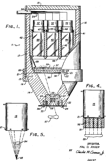
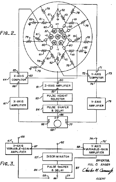
The decay mode of the radiopharmaceutical normally determines the gamma-ray detector to be used. In the simplest case, exactly one photon is produced. This mode is suitable for -scintigraphy or SPECT. If the radionuclides disintegrates via -decay, it is nearly instantly followed by collinear -photon pair emerging from the positron-electron annihilation. Whilst this radiation can be used for each of the three modalities PET, SPECT and -scintigraphy, its is particularly well suited for coincidence imaging. Certain radionuclides emit two gammas of different energies in cascade (, , and ) or one gamma and a positron like , and electron capture is known to give rise to X-ray and radiation ( and ). This opened up the possibility for - coincidence tomography, as proposed by Powell and Mohan in 1970 and 1970. Once again, the radiation resulting from these decay mode can be imaged with PET, SPECT and -scintigraphy. As a consequence of the arguments and examples above, nuclear imaging is essentially based on -ray imaging and the energy of the emerging -photon is a further important parameter that has to be taken into account for the construction of the imaging detector. Due to the quantum nature of photons, they cannot be partially stopped by the detector material. It either comes close enough to an atom to undergo one of the possible elementary interactions or it will not be affected at all. The probability for the interaction strongly depends on the energy of the -ray, on the effective atomic number of the atom and the density of these atoms (or compounds) forming the detector material. That is to say, the -imaging detector has not only to detect the photon, but also has to stop it for detection. The ability of the detector to stop the -ray is known as its intrinsic efficiency. This is the reason why Anger-type -cameras, optimized for 140 keV radiation from the tracer will only produce low quality images when used for SPECT with 511 keV annihilation radiation. However, efficiency is not the only parameter of interest and its optimization is very often in conflict with the optimization of others.
PET, SPECT and -scintigraphy are now widely applied to medical diagnostics and research in the fields of Cardiology, Oncology and Neurology. They are sometimes referred to as molecular imaging, since being photon-counting methods, they are actually able to visualize single molecules. It is that striking sensitivity that makes them very useful for the evaluation of biological systems that are particularly sensitive to small quantities of metabolic active substances such as many receptor systems and intracellular processes. Compared to MRS, which requires concentrations of paramagnetic tracers of mol/l in order to change relaxativity, the normally administered concentrations of is with mol/l four orders of magnitudes smaller. Iodinated contrast agents even need a concentration of mol/l to achieve opacification with X-ray CT (Blankenberg et al. [Blankenberg:2002]). As a result, for the moment only nuclear imaging allows the in vivo uninfluenced study of certain specific biochemical, physiological or metabolic processes, since the normally administered concentrations will not cause a pharmalogical effect.
1.2 Gamma-Camera (Planar Imaging)
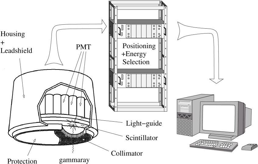
The principle of the Anger-type scintillation camera which was presented by Hal O. Anger in 1958 (Anger [Anger:1958], refer to figure 1.3) has changed little in the past half century and is based on the “camera oscura” from the early days of photography. While this principle was replaced by sophisticated optics in photography, it is not possible to construct lenses for -radiation except for some special cases. Figure 1.4 shows a schematic diagram of an Anger-type gamma-camera. The object to be studied is placed in front of the device, and, after the injection of the radiopharmaceutical, is continuously emitting -radiation. Although a large fraction of radiation is lost due to isotropic emissions, absorption by the collimator or because it is not absorbed by the scintillator, there are still sufficient -photons that interact with the scintillator. The -photons that interact with the scintillation crystal will originate isotropic scintillation light whose spatial distribution is projected through the light-guide onto the sensitive area of the photodetector. This distribution is sampled by the photodetector array or a position sensitive photodetector and used to compute electronically the position of the impact within a plane within the scintillation crystal and normal to the detector axis. In order to protect the detector from environmental and backscattered radiation, it has to be fitted into a shield. Modern gamma-cameras occasionally wrap the photodetector into -metal to protect it from external magnetic fields. Furthermore, the holes of the collimator have to be covered to avoid diffuse straylight to be detected by the photodetector. In general, this is done with an aluminum sheet of small thickness that does not stop the -radiation.
While this principle is repeated in almost all gamma-cameras, there exist clear differences from one camera to another depending on the components used and the applications that they are designed for. If the object as well as the scintillation crystal is large, e.g. for a whole-body scan of a human being, the pinhole collimator leads to an important loss of sensitivity and the use of a multiple hole collimator is advised (Anger [Anger:1964]). The main differences of these two collimator types are their field of view (FOV) and their efficiency. The FOV of the parallel hole collimator (figure 1.5(a)) is just its spatial extension parallel to the source plane and is independent of the distance between object and collimator.
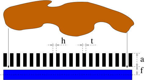
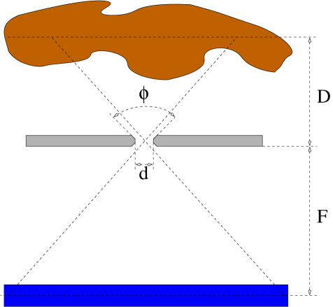
In the case of the pinhole collimator (figure 1.5(b)), the FOV depends on the distance between object and collimator. It can be approximated using pure geometrical arguments as follows:
| (1.1) |
where is the effective area of the scintillation-crystal photodetector combination and its distance to the collimator. The geometric efficiency is given by
| (1.2) |
where the effective pinhole diameter accounts for effects due to near-hole collimator penetration of the -rays and is the collimators absorption coefficient for the -ray energy of interest. Clearly the geometric design of the pinhole collimators also contributes to the total spatial resolution of the camera by
| (1.3) |
where is the scintillation detectors intrinsic resolution. For a circular parallel hole collimator, the geometric efficiency is given by
| (1.4) |
where denominates the area covered by one aperture, is the area of the whole collimator, the number of the apertures and the thickness of the collimator. Its contribution to the spatial resolution can be approximated by
| (1.5) |
It is clear from the equations 1.1-1.5 that type and quality of the collimator is of striking importance for FOV, spatial resolution and detection efficiency.
1.3 Single Photon Emission Computed Tomography
When the Anger-type gamma-camera is rotated step-wise around the patient while acquiring projection images at each step, a tomographic image can be reconstructed from a sufficiently large set of projections. Today this is known as Single Photon Emission Tomography or Single Photon Emission Computed Tomography. The spatial resolution of the resulting images depends on the performance of the gamma-camera used and is thus comparable to the resolution of the planar gamma-ray imaging modality. However, the contrast is significantly increased compared to planar imaging leading to more reliable lesion detectability. The sensitivity of SPECT is clearly outperformed (by approximately two orders of magnitude) by Positron Emission Tomography and also its spatial resolution falls behind because it is strongly affected by the necessity of collimators. Nevertheless, SPECT is an imaging technique nowadays widely used in medical diagnostics and the reason for this is that SPECT devices currently used for clinical purposes consist of from one to three Anger-type gamma-cameras. Thus, unlike PET scanners, SPECT scanners are multi-modality devices and allow for a higher cost-effectiveness and broader field of application. Historically, SPECT was introduced into nuclear medicine facilities by upgrading existing gamma-cameras and using the same radiopharmaceuticals. For this reason, there was no need for expensive compact cyclotrons and radiochemistry facilities for tracer production, although the low -ray energy give raise to a large fractions of Compton scattered events and totally absorbed -photons. It is therefore far from being ideal for tomography of the human body but remains an interesting imaging modality for small animal studies, where it is commonly used in experimental oncology (Weissleder [Weissleder:2002]).
1.4 Positron Emission Tomography
Positron Emission Tomography is often referred to as the benchmark technique for functional imaging. At the same time, it presents the highest level of resourcing for in vivo studies among all inherently contrast agent imaging modalities. In 1950, Gordon L. Brownell suggested that spatial resolution and sensitivity of nuclear imaging of brain diseases might be improved using annihilation radiation (Brownell [Brownell:1999]). PET is based on the decay of a emitting radioisotope tagged to a derivative of a metabolic active substance. The released positron has only a very short lifetime after the decay of the radiotracer and its path ends in an annihilation with one of the millions of surrounding electrons. As a consequence of energy and momentum conservation, the annihilation process gives rise to the nearly collinear -photons with an energy of 511 keV (refer to figure 1.6).
If both -photons are detected, the two points in space where they are detected define a straight line, the line of response (LOR), which necessarily contains the annihilation point. Since the path of the -rays is known, there is no need for absorptive collimation of the tracer radiation which is necessary in planar imaging like SPECT. Consequently, PET offers a wide acceptance angle for detecting the -photons and its sensitivity of approximately mol outperforms the sensitivity of SPECT by two orders of magnitude (Cassidy et al. [Cassidy:2005]) and, that of a single headed Anger-type camera by three orders of magnitude (Jones [Jones:1996]). In addition, the temporal coincidence detection provides an inherent and efficient rejection of background radiation and a further advantage is that the higher energy of 511 keV of the annihilation radiation entails a much higher probability for the -rays to escape from the examined object, which is not the case for the 140 keV radiation normally applied with SPECT and -scintigraphy. While for a 140 keV photon the half-layer of soft-tissue (International Commission on Radiation Units and Measurements, Four-Component soft-tissue) is , this value reaches for 511 keV radiation. It is therefore no surprise that, within the spectrum of nuclear imaging, PET is the modality par excellence for qualitatively and quantitatively imaging molecular pathways and interactions in vivo.
However, annihilation coincidence detection does not present a miracle cure for the physical problems of nuclear imaging and also involves fundamental problems. First, the higher penetrating power of 511 keV -rays not only is true for the examined object, but also applies to the photon-detector. One of the fundamental principles of Quantum Mechanics requires the -photon to be stopped and destroyed in order to detect its path and energy. Due to the greater penetrating power of the annihilation radiation, the detector has to be more massive and normally of larger dimensions. Another drawback is that both annihilation photons have to be detected to register a counted event. This directly translates to a quadratic dependency of the tomograph’s detection efficiency on the intrinsic detection efficiency of one detector module. Furthermore, since there are now two -rays that have to escape from the examined object, both of them can undergo Compton scattering and the probability of misspositioned events is also squared.
\psfrag{t}{$\mathrm{\tau(d,\omega)}$}\psfrag{A}{$\mathrm{A}$}\psfrag{d}{$\mathrm{d}$}\psfrag{w}{$\mathrm{\omega}$}\psfrag{t1}{$\mathrm{\tau_{1}(d_{1},\omega)}$}\psfrag{A1}{$\mathrm{A}_{1}$}\psfrag{d1}{$\mathrm{d_{1}}$}\psfrag{t2}{$\mathrm{\tau_{2}(d_{2},\omega)}$}\psfrag{A2}{$\mathrm{A}_{2}$}\psfrag{d2}{$\mathrm{d_{2}}$}\includegraphics[height=69.63402pt]{introduction/pet-geo-eff}
\psfrag{t}{$\mathrm{\tau(d,\omega)}$}\psfrag{A}{$\mathrm{A}$}\psfrag{d}{$\mathrm{d}$}\psfrag{w}{$\mathrm{\omega}$}\psfrag{t1}{$\mathrm{\tau_{1}(d_{1},\omega)}$}\psfrag{A1}{$\mathrm{A}_{1}$}\psfrag{d1}{$\mathrm{d_{1}}$}\psfrag{t2}{$\mathrm{\tau_{2}(d_{2},\omega)}$}\psfrag{A2}{$\mathrm{A}_{2}$}\psfrag{d2}{$\mathrm{d_{2}}$}\includegraphics[height=69.63402pt]{introduction/pet-geo-eff-coin}
The overall sensitivity of PET is determined by the intrinsic detection efficiency of the detector system and the fraction of the solid angle that is covered by the detector. The latter is called the geometric efficiency and is normally a nontrivial function of the detector’s and FOV’s geometry. Actually, the distinction between and is hard to clearly define. This is due to the fact that one has to stop the impinging -ray in order to detect it, i.e. a non-vanishing detector volume is required and consequently the detector element’s geometry is already involved. For one single detector element, one can compute its efficiency by
| (1.6) |
where is the area of the detector facing the radiation source, the distance of this surface from the source, the solid angle as shown in figure 1.7(a), the linear absorption coefficient of the detector material and the length of the path of the -particle through the active detector volume. Likewise one finds for the efficiency of an annihilation coincidence detector
| (1.7) |
In order to obtain the total efficiency, equation (1.7) has to be multiplied by a factor that represents the fraction of the spherical surface occupied by and . Furthermore, one has to take into account that the examined object also absorbs -photons. The angular dependency is, however, highly nontrivial because it also depends on the density distribution of the examined object, normally an animal or a human. Approximately, one can write the coincidence detection efficiency as (Cherry et al. [Cherry])
| (1.8) |
where is the (mean) absorption coefficient of the examined object and its total thickness. Instead of , the average geometric efficiency
| (1.9) |
is frequently used. This expression is valid when the detector dimensions are small compared to the distance between both detectors. The factor 2 in the numerator accounts for the fact that if one -photon is detected, the second photon inherently points towards the second detector module. The factor 3 in the denominator is the average coincidence detection efficiency across the sensitive volume at mid-plane. Commercial state-of-the-art PET scanners typically arrange up to 18000 small detectors in circular or (regular) polygonal arrays. Each detector element operates in multi-coincidence mode with a very large number of the opposite detector elements. If a perfect ring-detector is supposed, i.e. a complete ring of very small detectors of thickness in axial direction, diameter with and vanishing inter-detector spacing of adjacent elements, one obtains for a point source located at the center of the ring by geometrical arguments
| (1.10) |
and
| (1.11) |
for the average geometric efficiency when moving the point-source axially away from the center plane of the ring towards its end-planes. Equations 1.10 and 1.11 are valid for a small volume element near the center of the ring and also apply to polygonal arrays and continuous detectors that use the Anger positioning logic.
The spatial resolution of coincidence detectors depends in a nontrivial way on the detector module’s intrinsic resolution. For the case of discretized detectors, it depends primarily on the size of the individual detector elements since there is no possibility to decide where within the element the -ray interacted. One can derive the functional dependency of the spatial resolution on the position along the interconnection line in the following way. Suppose, an ideal point source is placed at the center between two ideal detectors. The distance between both detectors is . If discretized detectors are used, the elements are normally all of equal size . Annihilation radiation in coincidence detection results in lines of response that are defined by the two interaction points within the crystal. Now, the source is moved along a plane between the two detectors and and parallel to their surfaces through the field of view of the coincidence detector (refer to figure 1.8). By doing so, one obtains the point-source response profile of the coincidence detector for that plane. This profile is the convolution of the geometrical projections of both detectors onto the plane where the point source is situated and with the center of dilatation lying within the plane of the opposite detector. Since the geometric projection depends on the position along the optical axes , the spatial resolution also does. At mid-plane (plane A) of the detector pair, two identical rectangle functions with width are convolved and the response profile is a triangle function with a FWHM of . As the source moves towards either detector, the response profile becomes trapezoidal (plane B) and a rectangle function of width at the face of either detector (plane C). For any plane in between, the FWHM of the response profile can be given as
| (1.12) |
and the mean spatial resolution as
| (1.13) |
The very same arguments hold for deriving the spatial resolution as function of the inter-detector position for the case of continuous detectors. If one assumes the intrinsic spatial resolution of both detectors to be equal and its response profile of Gaussian form, then the convolution of their projections is also a Gaussian. One obtains the standard deviation of the resulting Gaussian by the geometric sum of the standard deviation of the both projected Gaussians. Thus the spatial resolution along is given by
| (1.14) |
and the mean spatial resolution by
| (1.15) |
1.5 PET Designs
The first PET systems were either two or more Anger-type cameras operated in temporal coincidence or used individual detector units consisting of a scintillator block coupled to a photomultiplier tube and arranged in one or multiple rings around the subject. This geometry required a huge number of the expensive photomultiplier tubes and as a consequence there was a large interest in multiplexing schemes that would reduces the number of PMTs. In 1984, Scanditronix designed a PET scanner that used detector modules of one PMT and two scintillators with different decay time (Nutt [Nutt:2001]). The crystal where the -ray is stopped could be identified by measuring the decay time of the current pulse. Only a few tomographs were produced and the technique was given the name of phoswich-detection333The word phoswich is derived from the words phosphor and sandwich.. It now carries the hope of enabling depth of interaction detection in -ray imaging. Burmham et al. at the Massachusetts General Hospital placed many individual photodetectors on a circular light-guide. By taking the ratio of two adjacent PMTs, the position could be estimated just in the way it is done in Anger-type cameras. Mike Casey and Ronald Nutt from CTI recognized the advantages of this method and developed finally the Block detector that significantly eases the manufacturing process and eo ipso reduces costs. Figure 1.10(a) shows the basic configuration. A large piece of scintillation material is partially segmented into many small elements. A variation in he depth of the saw cuts from element to element is used to control the distribution of the scintillation light to the four single-channel photomultiplier tubes. Two position estimates and can be computed from the four signals by simple arithmetic operations:
| (1.16) | |||
| (1.17) |
which are used afterwards to identify the element where the scintillation light came from. Typical Block detectors are made from 20 to 30 mm thick BGO or LSO with 4 to 6 mm wide sub-elements. While the first Block detector used only 32 crystal elements, up to 144 crystals per PMT can be found in modern state-of-the art PET scanners.
\psfrag{Cuts}{\footnotesize Saw cuts}\psfrag{PMTs}{\footnotesize four PMTs}\psfrag{Scintillator}{\footnotesize Block of Scintillator}\includegraphics[height=78.76865pt]{introduction/block-detect-commented}
\psfrag{Cuts}{\footnotesize Saw cuts}\psfrag{PMTs}{\footnotesize four PMTs}\psfrag{Scintillator}{\footnotesize Block of Scintillator}\includegraphics[height=78.76865pt]{introduction/partial-ring-scanner}
\psfrag{Cuts}{\footnotesize Saw cuts}\psfrag{PMTs}{\footnotesize four PMTs}\psfrag{Scintillator}{\footnotesize Block of Scintillator}\includegraphics[height=78.76865pt]{introduction/vollring-scanner}
\psfrag{Cuts}{\footnotesize Saw cuts}\psfrag{PMTs}{\footnotesize four PMTs}\psfrag{Scintillator}{\footnotesize Block of Scintillator}\includegraphics[height=78.76865pt]{introduction/planar-scanner}
\psfrag{Cuts}{\footnotesize Saw cuts}\psfrag{PMTs}{\footnotesize four PMTs}\psfrag{Scintillator}{\footnotesize Block of Scintillator}\includegraphics[height=78.76865pt]{introduction/hexagonal-scanner}
The geometry of dedicated PET-systems is strongly confined by the facts that temporal coincidence detection is required and that sectors without -ray detection result in artifacts due to the image reconstruction methods used (Natterer and Wübbeling [Natterer]). Therefore, one finds either closed ring and regular polygon systems that exhibit a clear axial symmetry or partial ring and polygon systems that are rotated in order to re-establish the broken symmetry. Figures 1.10(b)-1.10(e) illustrate some different approaches. Especially in PET scanners with circular geometry one often finds several stacked full rings in order to increase the axial FOV. PET scanners with a polygonal arrangement of panel detectors normally inherently exhibit a sufficiently large axial FOV. Further advantages of full-ring systems are a higher efficiency and reduced scanning time. In particular the gain in efficiency has to be mentioned since it grows with the square of the active detecting volume when no septa are used. Suppose one has a system consisting in one single detector ring. If one now adds a second full ring, one not only gains the events detected by this new ring, but also those events where one -photon is detected by one ring and the second by the other.
1.6 Radioactive Agents and Nuclear Medicine
The very first study of metabolism using radioactive substances transport within living systems dates back to 1923, when de Hevesy and Paneth investigated the transport of radioactive lead in plants. Seven years after, Ernest Lawrence et al. constructed the first cyclotron (Bryant [Bryant:1993]) with the aim of bombarding elements and exploring the nature of the atomic nucleus (Wagner [Wagner:1998]). It took further 4 years until Curie and Joliot discovered that elements could be activated by irradiating them with alpha particles from radium or polonium. The importance of the radiotracer principle together with the fact that virtually every element could be activated now became clear, and in 1935 Hevesy and Chiewitz were the first to apply this new principle to a study of distribution in rats. In 1936, Martin David Kamen came to Berkeley to visit Lawerence’s famed radiation laboratory. He was finally hired and used the cyclotron to produce the radioactive in order to clarify the still poorly understood process of photosynthesis. However, the usefulness of this isotope was limited by its very short half-life of only 21 minutes that forced Kamen and its colleagues to work at high speed and even to use carrier pigeons to interchange samples between laboratories. The discovery of with its half-life of 5730 years was the result of the search to find a more suitable radioactive carbon isotope. This isotope is very important because it can be used for determining the age of fossils as shown by William Libby in 1946. Until the development of CT and MRI, nuclear medicine physicians focused their attention to the imaging of organs, which were insufficiently differentiated by X-ray imaging. However, the overwhelming potential of radiotracer imaging lies in its possibility to mark and trace virtually every metabolic active substance allowing a graphical representation of its distribution within the examined object. Thus the development of radiopharmaceuticals was focussed on biological elements like , , and that could be generated with cyclotrons.
One of the first in vivo studies was the measurement of cerebral blood flow with and later and . With the emergence of the Anger-type camera and detectors for positron-emitting radionuclides in 1953, the in vivo localization of tumors became possible. In 1960, Stang and Richards from the Brookhaven National Laboratory, USA, announced the new radionuclide , obtainable from and Paul Harper at the University of Chicago realized that it was almost ideal for nuclear imaging for various reasons: Its decay energy perfectly matches the requirements of Anger-type cameras. Its physical and biological half-life was short enough to allow administration of high doses and it was readily available through its long-living generator . Owing to its properties, became the workhorse of nuclear medical imaging. Decades elapsed before chemical analogues of interest could be tagged with radionuclides and even nowadays many radioactive tracer substances in routine diagnostic imaging are of a very basic chemical structure and often do not exist naturally in the human body. The renaissance of the biological radionuclide began with a study of Ter-Pogossian and Powers in 1958 on the oxygenation of tumors. They worked with and mice with mammary adenocarcinomas. Directly connected to -metabolism one finds the different saccharides as important energy substrates in living organisms explaining the high interest in a radiotracer that could visualize this metabolism. Of special interest is glucose owing to its importance as an energy pool for the nervous system. Since an adult human requires at least 180 grams of glucose every day (Ruhlmann [Ruhlmann]), standard scintigraphy could not be used due to the high signal level. Another inconvenience of this molecule was that it could not be labelled with one of the usual radionuclides known at that time. A first attempt was made in 1977 by Sokoloff et al. using -deoxyglucose. Deoxyglucose (DG) is an analogue of glucose in which the hydroxyl group on the second carbon has been replaced by hydrogen (Phelps [Phelps]). DG has also been labeled with the positron-emitting thereby making it accessible to positron emission tomography. The much shorter half-life of only 20 min. allows repeated studies in a single day, but unfortunately the DG’s blood pool clearance only takes about 40 min. Attempts were also made with -glucose, that is, using the radioactive labeled natural substrate glucose. Unlike the analogue tracer, labeled substrates cannot usually be used to isolate single reactions steps. In the case of glycolysis, the metabolic process in which glucose is converted to pyrovate444Pyruvate is the compound to start the energy cycle within cells that yield direct precursors to ATP or ATP itself., ten different chemical reactions are involved. The -labeled glucose undergoes a substantial fraction of these reactions and the following ATP-metabolism until it is removed from the cell as or -labeled lactate. It is clear that the radiation from these end-products cannot be distinguished from radiation coming from the tracer in its original form. Further, labeled intermediates could also be taken up by other processes completely different for glucose. The kinetic data is thus distorted and less reliable. By substituting the hydroxyl group on the second carbon of glucose by one obtains []-FDG. This radiotracer has a more suitable physical half-life of 110 min. and furthermore provides the advantage that its glycolysis breaks down after a few chemical reaction inside the cell. The idea for this tracer was born at a wine-tasting event where Lou Sokoloff and Martin Reivich coincided. They commented on their findings to Al Wolff and Joanna Fowler from the Brookhaven National Laboratory, where -labeled FDG has been synthesized for the first time by Ido et al. The first images using this tracer in the brain were taken with the Mark-IV scanner by Kuhl et al. and numerous later studies have been realized with []-FDG making it the prime radiotracer for routine medical PET explorations. Studies that were carried out with this radiotracer over decades have demonstrated the accumulation of []-FDG in cancerous tissue and showed that PET is very useful for different clinical requirements, such as detecting primary sites of cancer, differentiating benignity or malignity of lesions, staging and grading the degree of malignity, planing and monitoring of the treatment and detection of recurrent diseases and metastasis.
Nuclear imaging modalities are now established as a powerful scientific and clinical tool for probing biochemical processes in the human body. Since the discovery of and the development of []-FDG, many other more specific radiotracers have been found and successfully applied. It finally leads to the emergence of nuclear pharmacy as a specialty practice and motivated a large number of research groups to search for further possible radiopharmaceuticals. At the moment, there is already a very large spectrum of specific pharmaceuticals which can be used for visualizing very particular aspects of the metabolism of diseases and the prospects of finding new ones are promising. Routine clinical application nowadays embraces above all oncology, nuclear cardiology, and neurology (Schlyer [Schlyer:2004], Acampa et al. [Acampa:2000]). Nevertheless, the most commonly used radiotracers are still very unspecific or do not exist in the human metabolism. Present and future developments are strongly focused on new radiotracers with high specificity and with adequate kinetic characteristics for quantitative analysis. This includes the development of radiotracers for imaging neurotransmitter systems, amino acid transport, protein synthesis, DNA synthesis and receptor imaging (Kim and Jackson [Kim:1999], Fowler et al. [Fowler:2003]). A list of commonly mentioned radiotracers together with the medical tests that they are used for can be found in Appendix A.
1.6.1 Requirement for Radiotracers
Molecular imaging is very promising for providing physiological or biochemical information for individual patients and, as has been mentioned before, is already becoming a routine diagnostic technique in medicine. Generally, an imaging tool for routine medicine has to obtain the results in a short time in order to be useful. Functional imaging also requires that the uncertainty in each measurement is smaller than the reconstructed contrast among different physiological states so that a change in these states can be easily detected. Consequently, radiotracers have to fulfill some important requirements in order to be suitable for molecular imaging, especially if they are applied in human medicine (Phelps et al. [Phelps], Hamilton [Hamilton:2004]). First of all, the tracer must be related predominantly to the process of concern, whatever this may be. Also it is necessary that the turnover time of the tracer within the specimen must be within the time window of the nuclear imaging modality. This second requirement includes many different aspects of the radiotracer and radionuclide, the scanner to use and the biological tissue and function that is imaged. The choice of radionuclide has to be made on the basis of providing the maximum diagnostic information together with minimum radiation dose to the patient. Therefore, the radionuclide must have a sufficiently long physical half-life in order to obtain sufficient statistics for medical images of reasonable quality and at the same time, they have to be short for a fast lowering of the dose that the patient receives. There are two processes that reduce the radioactivity inside the patient once the radiopharmaceutical has been administered. Beside the radioactive decay, the radionuclide is removed from the body physiologically with a biological half-life . The effective half-life is the inverse sum of and . The pharmaceutical is also required to be non-toxic in the administered amounts, to be present in the target tissue in a sufficiently short time and the uptake in pathology should show differences from normal. Moreover, many of the radiopharmaceuticals are synthesized in situ and just before they are administered to the patient. This requires that the synthesis and the imaging process must be finished within a time frame that is compatible with the effective half-life of the radiopharmaceutical. Synthesis and imaging may take few minutes up to hours.
Generation
Radiopharmaceuticals can be divided into two categories by their properties whether they are brought ready for use from outside the site of application or whether they have to be reconstituted in situ. The earliest method of producing commercial artificial radionuclides was to expose a target material to the neutron flux of nuclear reactors. However, even in intense neutron fluxes only a very small fraction of the target nuclei is activated. Since the target and product nuclei are different isotopes of the same elements (neutrons carry no charge), they cannot be separated chemically. Hence, the product is not target- or carrier-free and of low specific activity. Carrier-free products can be generated by choosing particular targets whose activation results in short-lived intermediate products. If the subsequent decay to the desired radionuclide includes a change in the element, chemical separation is possible. Alternatively, radionuclides can be obtained by using particle accelerators, especially compact cyclotrons. Since the accelerated particles are charged, the product is normally a different element and can be separated chemically for obtaining carrier-free radionuclides.
A very important concept for obtaining radionuclides is the production of a long-lived generator. The principle consists in the creation of an unstable but long-lived parent radionuclide at the production facility. This parent decays steadily to produce a short-lived daughter nuclide which has all properties of the desired radionuclide and moreover whose chemical characteristics allow for easy separation. Examples for generators are , and . They decay to the radionuclides , and with the half-lives of 67 h, 4.7 h and 115 days respectively.
Chapter 2 Motivation and Outline
Those who fail to learn the lessons of history are doomed to repeat them.
NUCLEAR imaging modalities not only have proven very valuable in the medical disciplines of oncology, cardiology, neurology, neuropsychology and cognitive neuroscience and psychiatry, but also play a crucial role in pharmacology. Due to their dedicated functional imaging techniques, it is not only possible to evaluate in preclinical trials new drugs very effectively in small animals but also opens the doorway to a much more sophisticated and function specific drug development. Moreover, nuclear imaging has significantly enhanced the ability to study animal models of diseases by enabling the continuous in vivo monitoring of disease development and rendering many necropsy studies unnecessary. The possibility of transgenic manipulation of mice emerged in recent years and led to a more detailed understanding of existing crosslinks between specific genes and molecular, cellular and organ functions. So-called Knock-out mice are now the basis for studying the physiology of the brain, heart and any other function. The perspectives for molecular imaging become strikingly clear if one bears in mind that this progress was made with imaging equipment of rather poor performance. Spatial resolutions above 1 mm, sensitivity of mere 5% and less for dedicated small animal PETs together with energy resolutions of about 15% made many of these results possible. It is against this background that many research groups all over the world are making a great effort to further improve all performance parameters. Unfortunately, many of these parameters constitute design conflicts and nearly all conflict with the requirement of low fabrication cost. Yet, one of the most important prerequisites for a widespread application of the developed technologies is a low initial outlay.
A main motivation for this work has been the reduction of fabrication costs, under the condition that a reasonable detector performance is achieved. The decision to use continuous, large-sized scintillation crystals has been taken for this reason. It avoids costly segmentation of the crystals which involves the loss of a substantial amount of material due to involuntary rupture and the saw cuts and requires either a rather tedious assembling or the installation of a robot. Likewise, the choice of using large-area position sensitive photomultipliers together with the center of gravity algorithm (CoG) is a direct consequence of this goal. The price per unit sensitive area of these devices is acceptable for use in dedicated small animal scanners and the analogically implemented CoG algorithm effectively reduces the number of required electronic channels. Unfortunately, electronic implementations of the CoG algorithm in its present form are not able to provide information about the depth of interaction (DOI) of the incident -ray. This leads to artifacts that considerably reduce the spatial resolution of the detector, especially for the PET modality where thick scintillation crystals are required for stopping the incident -ray effectively.
In order to fulfill the precondition of reasonable detector performance, important enhancements of the analogue CoG algorithm become necessary. The known fact of the correlation between the width of the scintillation light distribution and the depth of interaction motivated the design of DOI enhanced charge dividing circuits and an algorithm for recovering the true impact positions from their output signals. For this purpose, a detailed comprehension of all aspects of light propagation within the scintillation crystal until its detection is indispensable and in chapter 4, the distribution of the scintillation light across the photosensitive surface of the detector is parameterized. In chapter 5, the behavior of existing charge dividing circuits is studied. It will be shown that all configurations analogically compute the trivial and the first non-trivial moment of the applied signal distribution and a novel modification will be presented that allows the simultaneous computation of the second non-trivial moment, which relates to the DOI. Chapter 6 briefly summarizes the impact of Compton scattering on the expected accuracy of the moment measurements. The results of chapters 4 and 5 have been verified by experiment. How this was done and what results have been obtained is explained in chapter 7. Chapter 8 presents a standard method on how the new information provided by the depth-enhanced charge divider circuits can be used to reconstruct the full, three-dimensional photoconversion position. The final chapter 9 summarizes the main conclusions and discusses the future outlook for this method.
Chapter 3 Detector Components and Limits
Every generation laughs at the old fashions, but follows religiously the new.
THE first radiation detector that was used in medicine was clearly the photographic film for X-ray transmission radiography. Film-based radiography is still used extensively in daily medical applications, a circumstance which is due to the high amount of structural information, the low cost and complexity and an outstanding spatial resolution of the photographic film. The overwhelming progress in atomic and nuclear physics caused an ever-increasing interest in more sophisticated and accurate particle detectors with constant improvement in spatial resolution, energy resolution, timing resolution, etc. In particular, the field of nuclear medicine benefits from these advances for obvious reasons.
Radiation detectors can be classified into three large families: Ionization detectors, scintillation detectors and semiconductor detectors. Ionization detectors were the first electrical devices that were developed for radiation detection. Members of this family are the ionization chamber, the proportional counter, the Geiger-Müller counter and later the multi-wire proportional chamber, the drift chamber and the time projection chamber (see for instance Leo [Leo:1994]). Except for very few cases, such as the HIDAC PET, developed by Jeavons et al. [Jeavons:1978], and a more recent proposal of using lead walled straw tubes (Lacy et al. [Lacy:2001]), none of these detectors are applied to medical imaging, mainly because it is difficult to design compact detectors. However, they are extensively used in experimental high energy physics since there is no need for compactness in large particle accelerator installations.
The most important detector design for medical imaging is the scintillation detector. They are undoubtedly the most versatile particle detectors with a wide range of applications. In 1903, Crooks invented the spinthariscope. This is probably the first use of scintillators for particle detection and consisted of a screen that produced weak scintillation when struck by -particles that could be observed with the naked eye. This, however, required some practice and it was tedious to use. After the success of Iams et al. in 1935 to produce the first triode photomultiplier tube, the human eye was replaced in 1944 by these new devices for the first time by Curran and Baker. The scintillation could now be counted using electronic devices. After further development and improvement of the photomultiplier tubes and the scintillators in the following decades, scintillation particle detectors are now among the most reliable and convenient detectors. This, and the fact that nowadays very compact scintillation detectors can be manufactured, leads to their wide application in medical imaging. Modern Scintillation detectors can provide information about the energy and two-dimensional position of the radiation. Moreover, they are very fast and, depending on the scintillator, can show very short recovery times compared to other types of detectors. With certain scintillators it is even possible to distinguish between different types of particles by means of pulse shape discrimination.
Semiconductor detectors are the youngest family of particle detectors. Real development of these devices began in the late 1950’s. They provided the first high-resolution detectors for energy measurement and were quickly adopted for particle detection and especially gamma spectroscopy. The use of semiconductors for position measurement is rather new, however development in this field has seen huge progress in recent years. This was mainly due to the adaption of technologies used in micro-electronics and has been further enhanced by enormous improvements in silicon detector technology, front end electronics and signal processing. Micro-strip detectors and silicon drift chambers exhibit excellent properties for use as high-resolution particle track detectors and are possibly the detectors for the next generation experiments in high energy physics. A very important drawback of semiconductor particle detectors arises from their intrinsic noise. Especially for imaging modalities that are based on high energy photons, this is an important design conflict. Due to the high energy of the photons, -ray detectors need to have an elevated stopping power which is achieved by sufficiently sensitive volume of high density materials with high effective atomic number. The density and effective atomic number are already determined by the choice of the semiconductor and only the volume remains as a free design parameter. Unfortunately, the noise of semiconductor devices scales with the volume and very strong constraints exist. Although the noise can be reduced by active cooling, this would further increase the cost of the system. Therefore there are very few and very specific applications that allow the use of solid state detectors in medical imaging.
3.1 Solid-State Gamma-Ray Detectors
The basic operating principle of semiconductor detectors is analogous to gas ionization chambers. The incident ionizing particle creates a large number of electron-hole pairs along its trajectory through the semiconductor material and these charges are collected by an electric field. Compared to gaseous ionization detectors, there are important advantages. In the case of semiconductor material, the average energy that is required to create a single electron-hole pair is , one order of magnitude smaller than the average ionization energy of for gases. Furthermore, semiconductors have a higher effective atomic number and density. Therefore the energy loss per traversed length is very large resulting in a high stopping power for ionizing particles. As a consequence, semiconductor particle detectors can be made very compact and the mechanical rigidity allows for building self-supporting structures. Despite the high material density, electrons and holes have a very high mobility and the charge can be collected in a few nanoseconds. Additional advantages are the possibility of embedding fixed-space charges for creating sophisticated field configurations and, as both detectors and electronics can be built out of silicon, they can be integrated in a single device (Lutz [Lutz:1995]). Important disadvantages are the already mentioned intrinsic noise that often makes intense cooling necessary and the possibility that their crystalline structure can be damaged by the detected radiation.
A simple - diode junction can already be used for the detection of light or ionizing radiation. The diode may be used without the application of an external bias voltage or in the reverse bias mode. Unbiased detectors are preferred for radiation level measurements. The example for a - junction in reverse bias mode is shown in figure 3.1. This is the common operation mode for single particle measurements. The diode consists of a very low doped substrate. In order to be able to collect the charges released by the radiation, metal contacts must be bonded onto both sides of the diode. Since simple contacts between many metals and semiconductors lead to depletion zones, highly doped but shallow and regions are introduced at both surfaces of the diodes before fitting the contacts. Electron-hole pairs that are generated inside the sensitive volume are separated by the electric field and will move towards the electrodes. For signal isolation purposes, the bias voltage is supplied to the - diode through a resistor.
Nearly all existing semiconductor detectors are based on this principle. More or less sophisticated modifications are made in order to achieve special required properties, such as position resolution, etc. Besides the elemental semiconductors and , there are composed semiconductors consisting of combinations of elements from different periodic table groups. Well known members of this family are and . In recent years, much investigation has been done in this field and the list of possible candidates is now very long and allows for choosing semiconductor materials that are most suitable for the application of interest. For instance, nitrides of the third group have high tolerance to ionizing radiation, making them suitable for radiation-hardened electronics. Among this large range, the II-IV semiconductor Cadmium telluride () and the II-VI ternary alloy semiconductor () are promising materials for hard X-ray and -ray detection. The high atomic numbers of the materials give a reasonable quantum efficiency that is suitable for operation at the energy range from to (Scheiber and Gaikos [Scheiber:2001]). These materials are already used in commercial devices for digital radiography, computerized tomography, small field-of-view -cameras and intra-operative probes for radio-guided surgery. However, large multi-element detectors made from these materials are very expensive which is still the main drawback of this technology.
3.2 Scintillation Detectors
The basic configuration of a scintillation detector is shown in figure 3.2 and consists of a scintillator that is optically coupled to a photosensor. As radiation interacts with the scintillator by elementary processes like Compton scattering or photoelectric effect, a knock-on electron is produced that then excites or ionizes the atoms and molecules of the scintillation crystal. The decay of these excited scintillation centers give rise to the predominantly visible light photons which can be converted to electrical signals with the photodetector.
3.2.1 Scintillators
Visual counting of the (at that time) recently discovered X-rays and also natural radioactivity became possible with the powdered phosphor materials and at the end of the 19th century and made possible the previously mentioned invention of the spinthariscope. Since that time, inorganic scintillators especially have been an integral part of medical imaging and are still heavily used in this discipline. This can be explained by their comparatively good detection efficiency for hard radiation. After the invention of the photomultiplier tube, the final breakthrough of scintillation detectors was due to the discovery of the pure and activated alkali halide crystals. In 1948, Hofstadter introduced the scintillators and for efficient photon and particle detection (Novotny, [Novotny:2005]). They have been used extensively for nearly 60 years and are still very commonly applied. Nevertheless, scintillator development is in full progress, and the volume of scintillator material required each year for medical imaging devices is considerable. All in all, a total of 175 tons of scintillator are produced annually (Moses [Moses:1999]).
Yet, the various nuclear medical imaging modalities differ in their underlying principles and above all in the energy of the -rays they have to detect. Therefore, there are different requirements for scintillation detectors and the scintillators to be used. An ideal scintillator must have a very large density and effective atomic number, high luminous efficiency (light yield), short decay time of the excited states, neither afterglow nor other background, and low cost. These requirements cannot be met by a single scintillator and many of them are still sub-optimal for many applications. This is essentially the reason for further research and development in this field. Since the all-in-one scintillator does not exist, one has to choose instead the most suitable from all available materials. Fortunately, the list of available scintillators is already rather long and the properties of the different materials cover wide ranges.
For developing a new scintillator material, materials with relatively high density, , and effective atomic number, , should be used because the absorption probability by photoelectric effect is proportional to (van Eijk, [vanEijk:2002]). The material should also be transparent to the scintillation light. Hence, crystals with a forbidden energy gap, , between valence and conduction bands must be used and clearly has to be large enough to permit the transmission of the light. This is fulfilled by ionic crystals or crystals with some degree of covalence. Also good energy resolution is required by many imaging modalities. Since the photon counting is dominated by Poisson processes, a large number of scintillation photons is desired and this is achieved by a low small forbidden gap. This is clearly a design conflict with the former requirement and a reasonable tradeoff has to be found. Further aspects are non-proportionality, crystal growth, photofractions etc. A list (which is not intended to be complete) of commonly mentioned scintillators together with their key properties is given in Appendix B.
The special requirements for X-ray scintillators are, in order of decreasing importance: high light yield, high density, good matching of the peak emission wavelength, well defined granularity and homogeneity. All these properties are nearly excellently combined by making it the universally used scintillator for this purpose.
For X-ray computed tomography, the most important property is low afterglow, followed in order of decreasing importance, high temporal and chemical stability and insensitivity to radiation damages, high density, good matching of the peak wave length and high light yield. and ceramic scintillators are often used here.
The requirements for Gamma-Scintigraphy and SPECT are already influenced by the higher energy of the imaged radiation. They are, in order of decreasing importance, high light yield for good energy and spatial resolution, high density for efficiently stopping the radiation, low cost because in general large quantities are required, good matching of the peak emission wavelength and short decay time. Almost all these requirements are well matched by the alkali halide crystals and . Recently, the new scintillators and have been introduced. These materials combine high light yield and good energy resolution with a response time much smaller than that of the former two crystals. Since their detection efficiency is comparable to that of , they may be interesting alternatives for future detector developments of this modality.
Finally, PET and PEM require above all crystals of a very short attenuation length, since annihilation radiation is already very penetrating. Further selection criteria, in order of decreasing importance, are short decay times of the excited scintillation centers, low cost because a high sensitive volume is necessary for a reasonable detection efficiency, high light yield and a good matching of the peak emission wavelength. Common scintillators for PET imaging are , (BGO) and (LSO). has long been the standard scintillator for Gamma-cameras and positron cameras for its high light yield and because it matches well the sensitivity of photomultiplier tubes. Moreover, it can be grown easily and large crystal volumes are possible. With the appearance of BGO in 1973, it was quickly replaced because BGO has significantly better stopping power and photofraction. However, light yield and energy resolution are far below the values obtained with . LSO was introduced by Melcher and Schweitzer in 1992 [Melcher:1992]. LSO achieves nearly the same detection efficiency as BGO having at the same time a much larger light yield and faster response. While there are different important drawbacks of this material, for instance afterglow (Rogers et al. [Rogers:2000]), radioactive background from Lu (Huber et al. [Huber:2002]) and poor intrinsic energy resolution, for the moment it is the scintillator of choice for the PET imaging modality. More recently, other LSO related scintillators have been developed. They are mixed lutetium silicate (MLS), (LGSO) and (LYSO). Other scintillators that have been used for PET detectors are (GSO), (LuAP) and (LuYAP).
3.2.2 Photodetectors
All designs of radiation detectors demand a component that converts the scintillation light into electrical signals. A large variety of detectors have been constructed during the past years and their different properties match a wide range of individual application needs. They can be grouped in vacuum devices, solid-state devices and a combination of both called hybrid devices and gaseous detectors (Renker [Renker:2004]). The latter group has been mainly designed for high-energy physics experiments and, up to now, there is no application of these devices for medical imaging in combination with scintillators. They will not be discussed here. Likewise, the group of hybrid photodetectors has no major significance for commercial nuclear medical imaging at present and they are not discussed here either.
All photodetectors have in common that the energy of the light photons is transferred to electrons and these electrons are detected. This process is called photoconversion. The groups of photodetectors differ, however, in which material is used and how exactly this energy transfer occurs. Normally, they also provide an inherent system of amplification that has to be adapted to the detector material used and to the kind of photoconversion that takes place.
A photon that impinges on the surface of any material can liberate an electron from its atom or even from out of the volume of the material of which the atom forms a part. This effect is called photoelectric effect and requires that the photon’s energy is higher than the electric work function of the material111The electric work function of a material is the minimum required energy for liberating an electron from the material volume.. Therefore, the work function defines the low energy limit of the light spectrum that can be detected when using a specific material. Typical photocathodes of photomultipliers have their threshold in the visible red light region. Semiconductors have a very low work function and thus can be used for detecting infrared photons. However, semiconductors also offer a second process for photoconversion. It is sufficient to lift a electron into the valence band and to avoid, by application of an electric field in an adequate way, that this electron recombines and can be collected. Due to the very low band gap of semiconductors, very little energy is necessary and a highly efficient photodetector can be realized.
Vacuum Tubes
After the discovery of the photoelectric effect by Heinrich Hertz in 1887 and its successful description by Albert Einstein in 1905, all conditions had been met for the development of the first photoelectric tube by Elster and Geiter in 1913 (see also Kume [Kume:1994]). The next milestone was the discovery of the compound photocathode called S-1 () which increased the sensitivity by two orders of magnitude and was the beginning of dedicated photocathode development.
Photoelectric tubes can be significantly enhanced by introducing secondary emission surfaces as was first mentioned in 1902. The photoelectrons are accelerated towards an additional electrode where their impact produces secondary electrons. In its first implementation by the RCA laboratories in 1936, only one additional electrode was used, but devices with more than one dynode were quickly developed. The repeated generation of secondary electrons results in an effective multiplication of the primary photoelectron and therefore an amplification of the signal. The implementation is very simple because the required vacuum tube was already realized with the simple photoelectric tube. Since this time, large progress has been made in the development of new photocathodes and different dynode types.
Modern photomultiplier tubes (PMTs) have a light transmitting window and a semi-transparent photocathode is normally evaporated directly onto the inner vacuum side of this window. Nowadays, there are also different types of windows with different properties such as cutoff wavelength, thickness and refraction index. Most often borosilicate glasses and UV-transmitting glasses are applied (Flyckt and Marmonier [Flyckt:2002]). The most used photocathode materials are the already mentioned silver-oxygen caesium, antimony-caesium (), and the bi- and trialkali compounds , and . Directly behind the photocathode, an input electron optics focuses all photoelectrons onto the useful area of the first dynode. Over the past 70 years, different dynode geometries and materials have been developed. The configuration of the dynode system has a very high importance for the achieved gain. Each single dynode has to be arranged adequately in order to allow the secondary electrons they emit to hit the following dynode. In PMTs with a typical number of 10-16 stages, gains of about are achieved. A number of dynode systems have been designed putting the emphasis on different key requirements. A very important property provided by mesh dynodes, foil dynodes and micro channel plate dynode is the low spatial dispersion of the electron avalanche. This allows position sensitive photomultiplier tubes (PSPMTs) that are now widely used for different imaging techniques. Circular cage dynodes allow for very compact and fast PMTs, but provide no spatial information.

Dynode materials must have a satisfactory secondary emission coefficient and a sufficient rigidity. Typical materials are , and . Their surfaces can be easily oxidized and yield , and which offer a reasonable secondary emission coefficient. For operation of the PMT, the dynodes have to be supplied with high voltages where the potentials of all dynodes must differ for correct acceleration and multiplication. This can be achieved with separate high-voltage supplies for each stage or using voltage divider known as bleeder circuits. Simple resistor chains normally show an insufficient linearity behavior, especially for high output currents. For this reasons, sophisticated and active bleeder circuits have been designed. An example for a high output linearity circuit is shown in figure 3.3.
The anode or anodes of photomultiplier tubes are the electrodes that collect all secondary electrons from the last dynode and provide the output signals. Its geometric configuration has to assure large collection efficiency, minimized space charge effects and good impedance matching with the following electronics. In position sensitive PMTs, pixelated anodes, crossed wire anodes or crossed plate anodes must be used.
An additional synchronous signal can be derived from the last dynode of the electron multiplier system. The requirement for such a signal often arises from the desire to synchronize different measurement instruments. Especially in the case of position sensitive photomultiplier tubes, the last dynode signal is of interest. Owing to the segmentation of the anode system, there is no signal that provides position independent information about the total amount of detected light. In order to obtain this information from multi-anode PMTs, all anode charges have to be summed up. This can be avoided by sensing one of the dynodes because the electrons for the avalanche are liberated from the dynodes and the sudden loss of many of them can be noted as a variation in the potential. To obtain an amplitude comparable with that of the anode, usually the last dynode is used for the derivation of the signal. Care has to be taken not to disturb the anode signal and an appropriate matching of the impedances must be assured. Otherwise, the anode signal will be distorted and the dynode signal differentiated respectively. The properties of this additional signal allows one to use it for the generation of trigger signals and also for hardware energy discrimination.
An important characteristic not only for photomultiplier tubes but all photon detecting devices is its quantum efficiency which gives the probability that an impinging photon leads to an output signal. A typical value for PMTs is 25%.
Solid-State Photodetectors
A very important advantage of semiconductor devices over photomultiplier tubes is their much higher quantum efficiency of about 80%. This reduces significantly signal noise caused by the Poisson process of photon detection. They can also be produced in a fully automated process and therefore can be cheap. It is also possible to make them very compact because there is no need for mechanical parts. At the same time, this makes them very insensitive to magnetic fields. The detector itself is only thick (Renker, [Renker:2004]).
The silicon PIN diode is an example of a semiconductor detector for visible light photons. Its functional principle has already been explained in section 3.1 about solid state -ray detectors. It can be produced by standard semiconductor processes and its operation is simple and reliable. However, it has no gain at all, making it only suitable for the integrating detection mode but not for single photon counting purposes. Arrays of PIN diodes are very easy to produce and the time response is, at 1-2 , quite low.
An important improvement of PIN-photodiodes are avalanche photodiodes (APDs). Theses devices are designed to allow a very high reverse bias voltage. For sufficiently high voltages, impinging light photons cause electron avalanches with achieved gains of between 50 and 200. Even higher gains are possible but they make the device very sensitive to ambient instability like temperature drift or residual ripple of the high voltage power supply. APDs are suitable for single photon counting and already have been successfully used for small animal PETs. Very interesting enhancements are large area APDs, (Shah et al. [Shah:2001]) position sensitive avalanche photodiodes (PSAPDs, Shah et al. [Shah:2002]) and solid-state photomultipliers (SiPMs, Petroff and Stapelbroek [Petroff:1989], Saveliev [Saveliev:2004]). PSAPDs consist of a large area APD covered with a thin layer with homogeneous resistivity. This layer performs an integration with linear weighting of the impinging light. From four currents extracted at the corners of the resistive layer, the centroids of the light distribution can be computed. Sensitive areas up to with a planar spatial resolution of are currently possible. Important drawbacks of all APD based devices are their high intrinsic electronic noise and the low temperature stability. Silicon photomultipliers consist of a large array of small APDs operated in Geiger mode. In this way, respectable gains can be obtained and their timing resolution of is also excellent. However, these devices are still under development and there is no commercial application in medical imaging to this day.
3.3 Degrading Factors
All modalities of nuclear imaging are limited by different physical effects and uncertainties that impact on their final performance, including all qualifying parameters like spatial resolution, noise and efficiency. In all modalities, namely PET/PEM, SPECT and gamma-scintigraphy, -photons are the information carrier and the detector modules are often of the same type, even though some of the design parameters differ. The detection of high and medium energy photons involves, however, a number of difficulties that are mainly due to non-ideal behavior of the detector components. Finite size of the detectors leads to a limited geometric efficiency, while the finite size of a detector pixel limits the spatial resolution. Likewise, none of the discussed radiation- or photodetectors have a quantum efficiency of 100% and all introduce electronic noise. Above all the signal to noise ratio (SNR) and the spatial resolution of the final image are degraded by a number of physical effects that are hard to avoid. Some aspects, e.g. efficiency of Anger-type cameras and positron emission tomographs, as well as the spatial resolution degradation caused by collimators, have been discussed already in sections 1.4 and 1.2 respectively and are therefore not repeated here.
3.3.1 Parallax Error and Depth of Interaction
One of the most important degrading factors for Positron Emission Tomography is the depth of interaction (DOI) problem. It is caused by the failure of nearly all -ray imaging detectors to provide full three-dimensional information about the photoconversion position within the scintillation crystal (or solid-state detector). As a consequence of its nature, it is inherent to all nuclear imaging modalities where the -rays enter the detector in an off-normal directions. The lack of DOI information leads to a parallax error in the determination of both remaining spatial direction. Its existence is known from other fields, especially from astronomy, where it is used for determination of stellar distances. Parallax is the Greek word for alteration and denotes the change of angular position of two stationary points relative to each other if the observer’s position alters. This is shown in figure 3.4. A Parallax error is introduced in -ray imaging whenever the thickness of the absorbing material is finite, the incidence direction of the -ray is oblique and only the spatial coordinates normal to the thickness of the detector are measured. Hence, the parallax error is due to the thickness of the detector and scales with the same. There is no parallax error for -rays whose angle of incidence equals 90° respect to the plane defined by both measured coordinates. For this reason, Anger-type cameras for scintigraphy or SPECT that use parallel hole collimators do not suffer from this error. Contrariwise, the pinhole collimator introduces parallax errors because it allows oblique -rays. The thicker the detecting material is, the larger will be the parallax error because the uncertainty in the depth of interaction increases. On the other hand one has the requirement of higher mass attenuation for increasing -ray energy. This can be obtained in two ways. The first way is the use of material with high attenuation coefficient and the second method is to increase the thickness. Therefore, the interaction depth uncertainty poses a more serious problem to positron emission tomography than to SPECT and to Gamma-scintigraphy with radiopharmaceuticals of low decay energy.
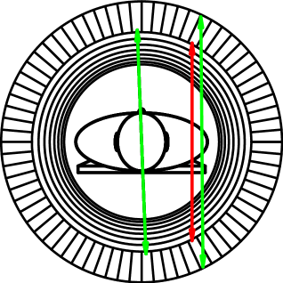
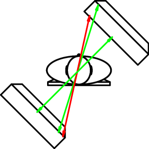
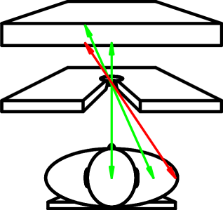
For the PET-modality, the parallax effect appears for any positron source displaced from the geometrical center of the tomograph’s field-of-view, or in general for any -ray impinging non-normal on the crystal (refer to figures 3.4(c) and 3.4(d)). Knowing neither the incidence angle nor the interaction depth, the incidence direction of the -ray cannot be unambiguously determined. In positron emission tomography, the parallax error is also known as radial elongation or radial astigmatism. For a typical commercial whole-body positron emission tomograph with wide detectors and a ring diameter of , the lacking DOI information reduces the spatial resolution by at a distance of only from the center of the field of view (Cherry et al. [Cherry]). Since the DOI effect increases strongly with the distance from this center, PET scanners are often designed with inner ring diameters much larger than it would be necessary to fit the patient.
Lack of interaction depth information leads to an additional positioning error when large-sized continuous scintillation crystals together with the center of gravity positioning scheme are used. This error is caused by the incomplete scintillation light collection near the borders of the detector. It leads to a strong, depth of interaction dependent image compression which is the main reason that nearly all research groups abandoned this particular design of PET detector modules. This particular error will be discussed in detail in section 5.8.
3.3.2 Compton Scattered Events and Randoms
Another very important error in emission tomography is the presence of scattered -photons. Although it is likewise caused by the inaccessibility of an important parameter, it is completely different in nature to the just discussed uncertainty. For all imaging modalities of nuclear medicine, it is necessary not only to detect -photons with energies between and , but also to determine information about their direction and line of flight. At these energies, -photons are very likely to undergo elementary processes like Rayleigh scattering, Compton scattering or photoelectric absorption within the detecting elements and also inside the explored patient, animal or tissue. Since the -rays are emitted isotropically, actually all surrounding matter, including detector housing, electronics etc., can cause scattered radiation. Since the photoelectric absorption destroys the -photons, they can no longer be detected and therefore only reduce the efficiency but, except for PET, do not lead to mis-positioned events. In positron emission tomography, two photons have to be detected. If one annihilation photon is absorbed before arriving at the detector element, no coincidence signal is possible and this event is lost as in the single photon case. However, the necessity of detecting two -photons can lead to the random coincidence detection of two different annihilation events when only one photon of each annihilation arrives at the detector. This leads to randomly positioned events.
Coherent (Rayleigh) scattering involves the interaction with an atom. Hence there is virtually no change in energy. Moreover, the scattering angles are usually low; that is, the original direction of the photon is only changed marginally. Compton (incoherent) scattering is an inelastic process that is due to interaction with the atomic and molecular electrons. In the energy range of relevance for nuclear imaging, especially PET, the probability of Compton scattering is high in all materials and tissue involved. Three types with different impact on the final image can be distinguished: Compton scatter within the explored body/tissue, Compton scatter within the detector but without detection by the same detector element (Back scatter) and inter- and inner-detector element Compton scatter. The last effect is of special relevance for the present work and will be discussed in detail in chapter 6. Back scatter includes large changes in the direction of the photon. The change in energy depends on the energy of the photon itself. While 180° scattered photons leave the interaction position with of their initial energy, photons will loose 2/3 of its energy under the same circumstances. Hence, in PET, one can effectively filter backscattered events by means of energy discrimination. Also, the detection efficiency of backscattering is normally low (Zaidi and Koral [Zaidi:2004]) and can be further optimized by means of adequate detector design. The impact of this scatter type on the final image is therefore normally low compared to Compton scattering within the region of interest (ROI).
Figure 3.5(a) shows the different types of mis-positioned events for single photon emission modalities. Clearly, the presence of collimators in single photon emission modalities reduces significantly the fraction of detected -photons that were scattered inside the ROI, but leads to additional mis-positioned events due to scattering within the collimator. Typical values for fractions of mis-positioned events in this modality are of the order of 5% when a based radiopharmaceutical (energy: ) is used and when a based radiopharmaceutical (energy: ) is used (Zaidi and Koral [Zaidi:2004]).
In annihilation coincidence detection, an event is registered whenever two events are recorded within a specified temporal window. True coincidences are those events that really arise from the pair of annihilation photons without intermediate scatter. Erroneous LORs can arise from a pair of annihilation photons when one of them or both undergo Compton scattering before being detected (event (2) in figure 3.5(b)). Also it is possible that two photons are detected (they may be scattered or not) from different annihilation events (event (3) in figure 3.5(b)). It is rather likely that one of the two photons of an annihilation pair is absorbed inside the ROI or fails to be detected by the system. The fraction of mis-positioned events is much larger in coincidence detection modalities because the -radiation is in general not collimated.222In many commercial PET scanners, passive collimation parallel to the plane of the drawing 3.5(b) is performed by septa. This is referred to as 2D-mode PET. If the septa are removed, it is called 3D-mode PET. Even with septa, all events in figure 3.5(b) can occur and there is actually no collimation for two spatial directions. Random events do not exist in single photon emission tomography.
An increase in scattered and random events results in a decreasing signal to noise ratio (SNR) of the reconstructed image. Even though the total of true events can be increased by designing detectors with higher efficiency, this would lead also to higher detecting efficiency for scattered events and randoms. In general, the different fractions and the final SNR depend in a complex manner on the geometry of the scanner, the detector element design and also the explored object (Humm et al. [Humm:2003]). For instance, Compton scattered events are of lower importance in small animal PET. In order to provide a physical measure for characterizing the influence of scattered events and randoms, the noise equivalent count rate (NEC) was introduced:
| (3.1) |
where , and are the count rates for true events, random events and single detected photons. Noise equivalent count exhibits a maximum when plotted against the administered activity. This is the activity at which an optimum SNR is expected.
3.3.3 Errors Contributed by the Radiopharmaceutical
Beside the limitations mentioned so far, Positron Emission Tomography has to deal with a further position uncertainty arising from the nature of the decay which was already shown in figure 1.6. In particular, this measurement error is caused by the range of the positron within the explored tissue (Phelps et al. [Phelps:1975], Palmer and Brownell [Palmer:1992], Levin and Hoffman [Levin:1999]) and the non-collinearity of the annihilation photons (Beringer and Montgomery [Beringer:1942], de Benedetti et al. [DeBenedetti:1950]).
Radionuclides that are used for PET have to be -emitters. They are nuclides with a proton excess and can decay by two processes:
| (3.2) | |||
| (3.3) |
The first reaction (3.2) describes the ordinary -decay. For this mode, decays directly to the ground states are possible. The second reaction (3.3) is the competing electron capture process.
In most cases, radiopharmaceuticals for PET are based on fluorine 18F, oxygen 15O, carbon 11C, and nitrogen 13N. The transitions of these radionuclides are allowed Gamow-Teller (18F) and allowed Fermi-transitions (15O, 11C, and 13N). Therefore, they exhibit the required short half-lives in the order of minutes as it was discussed in section 1.6. Decay schemes for these radionuclides are displayed in figure 3.6. Since for -decay the positron is always accompanied by a hardly detectable neutrino that shares the momentum and energy, the energy spectrum of the positron is continuous.
After the decay process, the positron loses energy since it interacts with the tissue until it finally annihilates with an electron and gives rise to the emission of two -rays propagating in nearly exactly opposite directions. The permanent collisions with the molecules slow the positron down and the annihilation in general does not occur until the is in thermal equilibrium with the environment. For this reason, the range of the positron strongly depends on its initial energy. This process can be described diffusively (Palmer and Brownell[Palmer:1992]) or alternatively by the Bethe-Bloch formula (Leo [Leo:1994]). Figure 3.7 shows the results for the distributions of the positron range in water and corresponding FWHM and FWTM values that were obtained by Levin and Hoffman [Levin:1999] from Monte Carlo simulations.
Besides the loss of spatial resolution in positron imaging devices caused by the positron’s range, there is a second equally fundamental effect, which in certain coincidence detector configurations can result in a more serious loss of resolution. After the thermalisation process of the positron, the kinetic energy of the annihilating pair is typically of a few eV which is mainly ascribed to the orbital momentum of the electron. In their center-of-mass frame, the photon energies are and their directions are exactly opposite. However, having a non-vanishing residual momentum, the two back-to-back -ray photons formed upon annihilation are not seen at exactly with respect to each other in the rest frame of the particle detectors (de Benedetti et al. [DeBenedetti:1950]). The angular spread leads to an approximately Gaussian-like distribution with the full width of at half maximum (Beringer and Montgomery [Beringer:1942]). For a system with a large detector-detector separation, this effect can result in a significant positioning error when reconstructing the location of the radiopharmaceutical. Both positron range and photon non-collinearity cannot be measured with present -ray imaging detectors and represent fundamental limitations to the spatial resolution of positron emission tomography.
3.4 Detector Improvements
Block detectors as discussed in section 1.5 made from BGO and LSO are still the most commonly used PET detector designs for commercial PETs. Typical performance parameters are detection efficiency, energy resolution, timing resolution and spatial resolution (Moses, [Moses:2001]). In the case of scintillation detector modules, the scintillation crystal poses the most important limit to the performance parameter. One important issue is to increase the very low total detection efficiency of usually for commercial PET scanner. This can be achieved by increasing the intrinsic efficiency of the modules or by increasing the total volume of the scintillation crystal. While the latter possibility is mainly a questions of costs, the first possibility together with high spatial resolution constitutes a pair of antagonistic design goals. This is because a higher intrinsic detection efficiency can only be achieved by thicker crystals or crystals of higher stopping power than BGO. For the moment, there is no alternative scintillator with higher stopping power than BGO and only the first possibility is left, but this would increase radial elongation as explained in section 3.3.1.
The timing resolution of scintillation detectors is mainly determined by the decay time of the scintillator. The shorter this parameter is, the higher will be the concentration of the detected light at the very first moments of the scintillation pulse leading finally to smaller statistical errors and a better temporal definition of the rising edge of the pulse. If the timing resolution of the -ray detector is sufficiently high, the possible positions of the positron’s annihilation point can be confined to a fraction of the FOV. This effectively increases the SNR of the acquired image. LSO is a very attractive alternative to BGO because it has a significantly faster decay time but nearly the same stopping power. Moreover, it has 3-4 times as much light yield compared to BGO and therefore allows for higher energy resolution and better definition of the detected position.
Developing PET detector modules with high timing resolution and the ability to measure depth of interaction information are two active fields of research. Notably, techniques of DOI measurement have mushroomed in recent years.
3.4.1 Depth of Interaction Detection
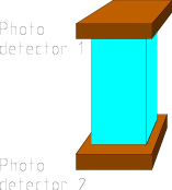
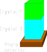
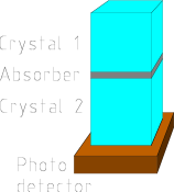
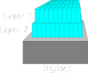
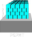
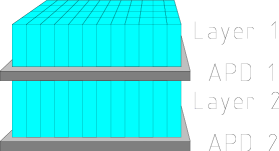
Detectors that do not provide information about the DOI of the recorded -ray introduce parallax errors which lead to uncertainties in the parameterization of the line of response (LOR) and, as a consequence, to a nonuniform and non-isotropic spatial resolution (Hoffman et al. [Hoffman:1989], Kao et al. [Kao:2000]). One possible strategy to partially overcome the effect of parallax errors is to restrict the transaxial field of view (FOV) of PET-systems to a small fraction at the center of the PET-system’s sensitive volume. Unfortunately this causes other unwanted effects such as loss of efficiency and an increasing relevance of photon non-collinearity, besides the fact that it makes compact PET scanners impossible. For existing -ray imaging systems, the image quality can be improved potentially if a sufficiently good estimate of DOI is provided by the detector. Especially for PET-detectors based on pixelated scintillators, a number of techniques for designing DOI capable detectors for -rays in the fields of nuclear medical imaging have been proposed. One of them consists in measuring the ratio of scintillation light detected at opposite crystal surfaces using two photodetectors and is shown in figure 3.8(a) (Moses and Derenzo [Moses:1994]). The DOI information is derived from the difference in the signal amplitudes of the upper and lower detector. To avoid additional expensive photodetectors and their associated electronics, other techniques can be used. Phoswich detector use pulse shape discrimination for DOI detection. Various layers of crystal pixels with different scintillation characteristics are stacked on a single position sensitive photodetector (refer to figure 3.8(b)). The DOI information is derived from measuring the pulse widths for the coincidence events (see for instance Seidel et al. [Seidel:1999]). Very similar to this approach is the introduction of absorbing bands between the different crystal pixel layers as shown in figure 3.8(c). This was also proposed by different research groups (Bartzakos and Thompson [Bartzakos:1991] and Rogers et al. [Rogers:1996]). A staggered double-layer array of crystal needles as displayed in figure 3.8(d) was proposed by Liu et al. [Liu:2001]. The relative displacement of the pixel layers allows the identification of the active layer by the detected transverse position. Similar to this method is the one proposed by Tsuda et al. [Tsuda:2006] and shown in figure 3.8(e). By introduction of vertical reflecting sheets between specific pixels and at different interfaces in each layer, the measured transverse positions are displaced by a well defined amount and allow for identification of the active layer. Completely independent crystal pixels have been proposed for the MADPET-II dedicated small animal PET scanner by Rafecas et al. [Rafecas:2001a]. This is shown in figure 3.8(f). Also combinations of different techniques are possible. However, all these approaches imply costly detector modifications to a greater lesser extent. They need additional photodetectors, smaller crystals or crystals of a different type.
Proposals for interaction depth measurements in continuous scintillation crystals for nuclear imaging were reported by Karp and Daube-Witherspoon [Karp:1987], Matthews et al. [Kenneth:2001] and Antich et al. [Antich:2002]. Except for Karp and Daube-Witherspoon, who used a temperature gradient applied to in order to force a variation of the signal shape with the interaction depth that could be used for discrimination, the other groups sampled the scintillation light distribution and computed the standard deviation from the data set because of its correlation to the interaction depth.
3.4.2 Time-of-Fight PET
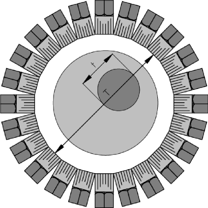
Commercial PET scanners have an inner ring diameter of . This distance is covered by a -ray traveling at the speed of light in . If the detector elements were able to estimate the time of arrival with this resolution, the supposed annihilation position can be restricted to a region of diameter and smaller than the disk defined by the PET scanner (refer to figure 3.9). The higher the timing resolution of the coincidence system is, the smaller will be the region from which the annihilation photons can originate. If this information is implemented in the reconstruction algorithm, the quality of the image can be improved significantly (Moses [Moses:2003]). One of the parameters that is improved is the SNR. But also the noise equivalent count rate is increased, because many random events can be now rejected. For a timing resolution of , the random rate is reduced by a factor 1.5-2, is increased by a factor 1.4-1.6 and the noise variance is lowered by a factor of 5.
Chapter 4 Parameterization of the Signal Distribution
Where there is much light, the shadow is deep.
IN chapter 2 it has been pointed out that the use of continuous scintillation crystals carries several general advantages and that good results can be obtained with -ray imaging detectors based on this design. When Positron Emission Tomography emerged as a novel imaging technology, it was straightforward to take the design from existing Anger-type cameras and use it for positron cameras, because they are just -cameras optimized for the detection of the annihilation radiation. The key problem arises from the high energy of this radiation. While -photons from the isotope have an energy of approximately , the energy of annihilation photons is more than three times as large. The detection of these photons presupposes the photoconversion within the scintillation crystal but the interaction probability decreases with increasing -ray energy. Therefore, the crystals have to be thicker in order to stop the same number of photons. Since it is not normally known at which depth the -ray interacts, an uncertainty is introduced. This may cause serious positioning errors for -rays with non-normal angles of incidence and, depending on which positioning method is used, depth-dependent variations in the position measurement. Apart from Anger [Anger:1963], there have been attempts by several research groups (Karp et al. [Karp:1985], Rogers et al. [Rogers:1986], Siegel et al. [Siegel:1995] and Seidel et al. [Seidel:1996]) to develop -ray detectors for positron emission tomography using continuous scintillation crystals instead of arrays of small crystal segments. Except for a few, all groups abandoned this design due to the strong border artefacts in large-sized continuous scintillation crystals caused by the center of gravity (CoG) algorithm (see section 5.8). Clearly, the crucial point is how the position measurement is implemented. The mentioned resolution degradation at the crystal edges is inherent in the CoG algorithm, but not necessarily in other positioning methods. There are statistical based position reconstruction schemes (Liu et al. [Liu:1990], Joung et al. [Joung:2002]) that do not suffer from this systematic error. However, a sampling of the signal distribution, i.e. the digitization of all channels, is required and the border-effects are avoided at the expense of higher computation time and detector costs. An alternative access to the real three-dimensional position where the photoconversion took place seems to be possible by using the width of the signal distribution, since this parameter is correlated with the interaction depth (Siegel et al. [Siegel:1995], Matthews et al. [Kenneth:2001], Takacs et al. [Takacs:2001], Antich et al. [Antich:2002] and Lerche et al. [Lerche:2005b]).
In this chapter, a parameterization for the density distributions of light seen by the photocathode and charge seen by the anode-segments of the position sensitive photodetector is derived. Although there are many simulation tools based on the Monte Carlo method, the analytic model was preferred, because it leads to a better understanding of the resulting distribution.
4.1 Included Contributions and Conventions
The signal distribution that is finally accessible for the reconstruction software emerges as an interplay of a broad variety of physical phenomena. The generation starts with the photoconversion of the incident -ray via a sequence of elementary interactions, e.g. Rayleigh scattering, Compton scattering and the photoelectric effect. However, only the position of the very first -ray interaction corresponds to the true line of response (LOR). The photoelectric effect and Compton scatter events produce so-called knock-on electrons that excite the atoms of the crystal material along its path until being completely stopped. Also, ionization with secondary electrons of high energy (-electrons) is possible. The scintillation light arises from the de-excitation of the scintillation centers along the different electron paths. Since common scintillators for PET are normally made of a high density material, these paths are rather short. One can estimate the range of these electrons using an empirical formula from Tabata, Ito and Okabe (Tsoulfanidis [Tsoul:1995]) based on experiments that measured the range of positrons by extrapolating the linear part of the transmission function and defining the intersection with the background to be the extrapolated range . The largest possible distance of is covered by an electron that emerges from a unique photoelectric interaction of an incident -ray and that produces no -electrons. However, the majority of produced electrons will travel much shorter distances before being stopped and we assume these elementary interactions to be point-like.
In this chapter, only signal distributions arising from single photoelectric interactions will be considered. This seems to be a very rough approximation, since for -rays one expects various Compton scattering interactions as part of the photoconversion even for dedicated PET scintillators such as LSO. The influence of inner-crystal Compton scattering on spatial resolution that can be achieved with the CoG algorithm will be discussed in detail in section 6. In section 7 it will be shown that even with this rigorous approximation, very good agreement with the real detector response is achieved. Signal distributions that arise from various interactions are superpositions of the independent single-event distributions. If the energies deposited at these points are different (as in the vast majority of the cases), the distribution arising from the point with maximum energy deposition will dominate.
Four issues have to be clarified before beginning with the derivation of the theoretical model. The first is the significance of continuous scintillation crystals. Crystals of almost every possible spatial dimension can be called continuous as long as one does not reach the molecular scale. Actually, the definition depends strongly on the scale, since a crystal of dimensions can be considered continuous, if the region of interest is confined to this same volume. The volume of interest for the present work is however defined by the product of the required scintillator thickness and the sensitive area of the photodetector. Throughout this work I will refer to a continuous crystal whenever this volume of interest is covered by one single crystal. Similarly, the expression pixelated crystal or crystal array is used, if the same volume is covered by several independent crystals. The second issue is the treatment of the crystal surfaces. Generally, only one of the six scintillator faces is coupled to a photodetector. For all other faces there exist many possible treatments that allow an optimization of the detector performance. However, the aim of the present work is not the detector optimization, and therefore, all free surfaces are assumed to be fine ground and covered by highly absorptive coatings in order to avoid reflections while the one that is coupled to the photodetector is assumed to be polished.
The third issue concerns the choice of the point of origin. Throughout the following sections and chapters the reference system is chosen in such a way that the sensitive area of the photodetector is parallel to the --plane and centered at the point of origin . The - and -spatial directions are understood to be the transverse and horizontal spatial directions respectively and the -direction the normal or vertical direction. The scintillator is placed within the half-space with and the detection material of the photodetector within the half-space with . The last issue is a pure naming convention. The expression depth of interaction (DOI) refers to the distance between the position of the -ray’s photoconversion and the crystal surface facing to the photodetector (refer to figure 4.1). For the derivation below, the distance between the photoconversion point and the crystal surface coupled to the photodetector is more intuitive. Throughout this work, this parameter will be primarily used and it will be called the interaction distance (ID).
4.1.1 The Inverse Square Law
The starting point for the derivation of the signal distribution is the inverse square law. It says that the intensity of light radiating from a point source is inversely proportional to the square of the distance from the source. This law is founded in strictly geometrical considerations and therefore applies to all isotropic radiation phenomena. It can be easily derived using the divergence theorem and gives
| (4.1) |
where is the amount of scintillation light at the observation point , is the total amount of released scintillation light and is the position of photoconversion. Equation (4.1) shows the geometrical character of the inverse square law since the denominator is just the expression for the surface area of a sphere with radius . Moreover, it states that the total number of light photons released at the scintillation center is conserved and does not change as the light propagates through the crystal.
4.1.2 The Cosine Law
In the previous paragraph, the inverse square was derived for spherical surfaces. Commercially available photodetectors offer always, except for a few special cases, a planar design of the sensitive area. Only for almost normal incidence of the scintillation light, the difference between planar and spherical surface element will be not very important. However, since continuous and large-sized crystals in the sense of section 4.1 are used in this study, a large fraction of the scintillation light impinges on the photodetector at large angles.
In the case of scintillation detectors, the position of the light source is confined to the volume of the scintillation crystal. For optimum performance, it has to be coupled through light guides as close as possible to the photodetector. Therefore, the normal distance between the light source and the photodetector never exceeds the thickness of the crystal. Furthermore, it is small compared to the planar extension of the detector. The photon flux corresponding to the surface element is covered by the detectors sensitive surface element as shown in figure 4.2. By similarity of the triangles spanned by and and and one deduces that
| (4.2) |
With this result, the inverse square law of equation (4.1) becomes
| (4.3) |
Equation (4.3) inherently has the correct normalization. Integrating over an infinite plane normal to the -unit vector and at , one obtains which is exactly the expected result since just the half of all released scintillation light will be collected.
4.1.3 Exponential Attenuation
While the scintillation light travels within the optical components of the detector, it is attenuated according to the exponential law
| (4.4) |
where is the inverse of the attenuation length at the wavelength , is the initial intensity and the attenuated intensity. An important requirement for scintillators is a high transparency to its own scintillation light in order to allow an effective light collection. Therefore, one can assume that is large compared to the spatial extensions of the scintillator. Otherwise, the chosen scintillation material would not be adequate for the application. Furthermore, can be approximated by the constant average value , since the emission spectra of many scintillators are confined to intervals of less than a few hundred with only small variations of over this interval.
4.1.4 Light Transmission to the Photodetector Window
The scintillation light that reaches the borders of the crystal is either absorbed at one of the five absorbing crystal sides or detected by the photodetector coupled to the transparent side. The photodetector itself contains a transparent entrance window for protection from environmental influences. Although this window is optimized with respect to collection efficiency and transparency, its refraction index in general does not match the one of the scintillation crystal. Furthermore, since the refraction index of the entrance window and the refraction index of the scintillator are much larger than the refraction index of air, air-gaps between both media have to be avoided. Optimal optical coupling is achieved with optical gel or silicone of intermediate refraction index. Hence, the scintillation light traverses an optical multi-layer system consisting of several homogeneous media in sequence, e.g. the scintillation crystal, the optical grease, the entrance window and the photocathode. There is also a fraction of light that is transmitted to the the vacuum if photomultiplier tubes are used for detection. The behavior of light at the interface between optical media of different refraction indexes is well described by Snell’s Law and the Fresnel equations. In order to reduce the complexity of the derived model-distribution, the intermediate layer of optical fat is not included in the considerations. This approximation can be made, since the refraction index is chosen to lie in between the values for the entrance window and the scintillation crystal, and because the thickness of the additional layer will be very small. Thus, it will cause only a very small deviation of the light path.
Refraction of the Light
The relationship between the angles of incidence and refraction for a wave impinging on an interface between two media is given by Snell’s law
| (4.5) |
where the angles and are taken with respect to the normal on the interface plane and and are the refraction indices of the scintillator and the entrance window respectively. The refraction index of inorganic scintillation crystals for -ray detection is comparatively high. is normally larger than . This leads to total reflection whenever the angle of the incident ray is larger than the critical angle . As a consequence, only the fraction of the scintillation light that is confined to the cone of aperture enters the photodetector and contributes directly to the signal distribution (Ambrosio et al. [Ambrosio:1999]). The scintillation light outside this cone is trapped within the crystal due to total reflection and most of it will be lost by absorption. The light inside the cone is refracted away from the normal on the interface. This is shown in figure 4.3.
For a photodetector, the sensitive material, i.e. the photocathode or the semiconductor will be located at the plane behind the window of thickness . Due to the refraction, light that is emitted from a scintillation event at the impact position will not be detected at the projected distance but at . The scintillation light seems to come from a point at normal distance from the interface instead of coming from point . One therefore has to compute as a function of the true interaction distance , the distance , the window thickness and . This is equivalent to find the roots of the following quartic equation:
| (4.6) | |||
Equation (4.6) has eight mathematical solutions but only one is of physical interest for the present problem. It is given by
| (4.7) | |||
| (4.8) |
With the aid of we can define the new, virtual photoconversion position . This is the position from which the scintillation light seems to come from. The dependence of on the projected distance from the impact position is shown in figure 4.4(a) for . In figure 4.4(b), the dependence of the angle of incidence of the light path on the detecting surface is shown for the same -values. At this point, important observations can be made. First, although the effect of total reflection prohibits the transmission of scintillation light into the photodetectors entrance window for certain angles, the light distribution seen at the detecting material will never be truncated. This is due to the fact that the light within the cone of aperture can pass to the medium of refraction index but will be refracted away from the normal onto the optical interface. For a light ray of incident angle , the refracted light would be bent in such a way that it propagates just within the plane of the interface. For all light rays with incident angles , the refracted angle will be in the interval . That is to say, the entering light which is confined to the cone of half-angle will be redistributed and causes a new continuous distribution illuminating completely the infinite plane at .
Another interesting phenomenon is that this resulting distribution is narrower than a light distribution without refraction. This effect was already observed by Tornai et al. [Tornai:1994] and is shown in figure 4.5(a) for the simple distribution (4.3). From the geometrical arguments in figure 4.3 one would intuitively expect that the light distribution observed at the detection material would be broader. However, the distribution is biased towards forward angles because increases more rapidly at larger for and consequently the photon density decreases with for larger distances (refer to figure 4.5(d)). Figures 4.5(b) and 4.5(c) show the behavior of the widths of both distributions for different IDs (and also DOIs). One can see that the FWHM of the distribution 4.3 depends linearly on the ID and that the detected width varies only slightly at around 80 % of the original width. For completeness, the fraction of detected light as a function of the critical angle for total reflection is shown in figure 4.5(e). Since the energy resolution of scintillation detectors depends strongly on the light collection efficiency, a good matching of the refraction indices and has to be achieved. A low light collection efficiency leads to larger statistical errors when the scintillation light is converted into electrical signals and consequently to a lower signal-to-noise ratio (SNR). This is shown in figure 4.5(f) for a hypothetical distribution of 2000 detected photoelectrons.
Fresnel Transmission
Apart from the refraction of the scintillation light path, reflection at the interface even for angles smaller than the critical angle are observed. Actually, Snell’s law only predicts the relationship between the angles of the incoming and the refracted light-path. The fractions of the intensities of incident light that is reflected from the interface and incident light that is transmitted to the second medium is described by the Fresnel coefficients for reflection and transmission .
| (4.9) | |||
| (4.10) |
Here the subscripts and specify the polarization of the incoming light. The light is called s-polarized if its electric field vector is normal to the plane spanned by the incoming light path and its normal projection onto the interface. If the electric field vector lies completely within this plane, the light is called p-polarized. Alternatively, these polarizations are often called transverse magnetic mode (TM) and transverse electric mode (TE) respectively. Scintillation light is not expected to be polarized along a specific direction but is supposed to be completely unpolarized. One therefore has to average over all possible polarizations thereby obtaining the fraction of light transmitted to the photodetectors window
| (4.11) |
where the refracted angle can be expressed as a function of
| (4.12) |
and the incidence angle can be obtained by virtue of Snell’s law (4.5), once the refracted angle is known.
4.1.5 Angular Sensitivity of the Photocathode
The physical effects considered so far, e.g. inverse square law, cosine law and optical transmission into the entrance window, are common to many different scintillation detector configurations. Also, the photodetector itself has a characteristic influence on the detected signal distribution because it is not an ideal device. Therefore, the type of photodetector used has to be specified at this point. For this work, a position-sensitive photomultiplier tube has been chosen as photodetector. A photomultiplier converts light into an electrical signal by photoemission of electrons from the photocathode. There are two main kinds of photocathodes: semi-transparent cathodes that are evaporated onto the inner side of the input window and opaque cathodes that are deposited on a metal electrode inside the tube (Flyckt et al. [Flyckt:2002], Kume, [Kume:1994]). Position-sensitive photomultipliers mostly use semi-transparent photocathodes because then the cathode can be very large and the entrance window on which it is deposited can be flat or curved. In this case, the photoelectrons are emitted from the side opposite the incident light.
Most photocathodes are made of compound semiconductors consisting of alkali metals with a low work function111The (photoelectric) work function is the minimum energy required to liberate an electron from the surface of the particular metal compound.. Often, the materials applied are silver-oxygen-cesium (), antimony-cesium (), Bi-alkali compounds (, and ) and the tri-alkali compound , besides the less frequent applied solar-blind types ( and ) and semiconductors of negative electron affinity and extended near-infrared sensitivity (, and ) (Flyckt et al. [Flyckt:2002], Kume, [Kume:1994]). Each of these photocathodes has its typical spectral response, which is, however, of less importance for the present derivation of the signal distribution. The quantum efficiency for photoemission not only depends on the wavelength of the incident light but also on the angle of incidence of the light. The dependence on this angle is called the angular sensitivity. It is mainly a consequence of reflections and multiple internal reflections inside the photocathode (refer to figure 4.6) and is therefore well described by a standard application of the Fresnel equations for reflectance and transmittance of multi-layer systems (Jones [Jones:1976], Chyba et al. [Chyba:1988] and Motta et al. [Motta:2005]).
The photocathode can be treated as a continuous medium with complex refractive index .222Complex refraction indices are used to describe absorptive media. It is deposited onto the photomultiplier’s entrance window of refractive index and faces the PMTs interior vacuum on the other side (). Calculating the reflectance and transmittance for a light beam incident from the entrance window on the photocathode one obtains
| (4.13) | |||
| (4.14) |
where
| (4.15) | |||
| (4.16) |
for s-polarized light (TM waves) and
| (4.17) | |||
| (4.18) |
for p-polarized light (TE waves). In addition, and
| (4.19) | |||
| (4.20) |
was used, where is the thickness of the photocathode and the vacuum wavelength of the incident scintillation light. Equations (4.13) and (4.14) have been derived and verified by various research groups (Jones [Jones:1976], Chyba et al. [Chyba:1988] and Motta et al. [Motta:2005]) and agreement with experimental data was found.
Neither the reflectance (4.13) nor the transmittance (4.14) are formulae of direct interest for the considered model for the signal distribution. Except for spurious reflections at the PMT’s dynode system and housing, and photoemissions at the first dynodes, the transmitted light does not contribute to the signal distribution. The reflected flux will also be neglected since we suppose our detector to have absorbing borders and therefore the major part will not be detectable. The scintillation light that will neither be reflected nor transmitted must have been absorbed by the photocathode and one has
| (4.21) |
Since the light is supposed to be completely unpolarized, one has to average equation (4.21) over all possible polarizations. Figure 4.7 shows a typical photomultiplier absorbance (4.21) and the different contributions for TE and TM waves.
4.1.6 Background Light
Besides the scintillation light that reaches the photocathode directly, there are also photons that are scattered or reflected. The contribution of the scattered photons is expected to be very small for reasons explained in section 4.1. However, the overall contribution of light reflected at the absorbing borders can become very important for different reasons. First, it is impossible to achieve ideal absorbing surfaces. Residual reflection is expected from all absorbing surfaces of the scintillation crystal. The total area of these surfaces is always larger than the area that is coupled to the photodetector. Secondly, if total reflection occurs at the entrance window, the ratio of reflected light to direct light even becomes more biased towards higher fractions of reflected light. Apart from this, we have Fresnel reflections at all optical interfaces.
A consequent inclusion of all possible contributions produced by reflection phenomena is clearly impractical. Instead, one has to look for a simple, computable model that satisfactorily describes the most important functional dependences of the distribution caused by reflections. Actually, an exact model is not even required because the distribution of reflected scintillation light is already a first order correction to the model. The following approximations are made:
-
Two or more successive reflections are neglected since they will be very improbable for black surfaces.
-
The black surfaces are supposed to exhibit ideal Lambertian reflectance. This assumption can be made since the crystal is only polished at the side that is coupled to the photodetector. All other surfaces are fine-ground and covered with a black epoxy resin composite of a very low reflection coefficient.
-
Light rays that undergo first a total reflection on the interface between the scintillator and the entrance window, and are subsequently diffusely reflected at one of the black-painted surfaces, are also considered because they are of the same intensity as light rays directly reflected at the black sides.
-
Fresnel reflected light from the different optical interfaces is not included. This would be already a second-order correction.
-
It was shown in section 4.1.4 that the refraction of the light leads to a narrower detected distribution when passing into the entrance window. We define as the effective window thickness that leads to the same average distribution width as the true refracted light distribution for the considered range of interaction distances. is used to approximate the effect of refraction of the background light.
The application of the inverse square law of equation (4.3) together with Lambert’s cosine law (Born and Wolf, [Born], Xu et al. [Xu:2003]) gives the four different contributions shown in figure 4.8. One has diffuse reflection at the crystal border
| (4.22) |
total reflection at the scintillator-window interface and subsequent diffuse reflection at the crystal border
| (4.23) |
with ; diffuse reflection at any of the crystal borders and
| (4.24) |
and total reflection at the scintillator-window interface and subsequent diffuse reflection at any of the crystal borders and
| (4.25) |
with . in equations (4.23) and (4.25) is the unit-step distribution and in equations (4.24) and (4.25) has to be replaced by or depending on the surface over which the integration is carried out. is the thickness of the scintillation crystal and its transverse dimension supposing a square shape. The complete background light distribution is given by the superposition of the contributions (4.22)-(4.25).
4.2 Complete Signal Distribution
The total scintillation light distribution is given as a superposition of the background light and the product of the contributions discussed in sections 4.1.1-4.1.5.
| (4.26) |
with
| (4.27) |
The subscript in (4.26) indicates that the light density does not only depend on the observation point and the -ray photoconversion position , but also on the scintillation detector configuration, e.g. the refraction indices, the entrance window thickness, the crystals spatial dimensions, etc. Sample distributions are plotted for different photoconversion positions in figure 4.9 with the following detector design parameters: , , , , , , , and . Also shown are the contributions of the background light due to diffuse reflection at the crystal borders. It can be seen that this contribution becomes important for large interaction distances and near the crystal borders and edges, while it is very low for small . Also the expected variation of the distributions width with the interaction distance can be observed. If the second moment and the standard deviation are computed from the distribution, the dependence can also be observed in this variables. However, both variables also depend on the planar impact position to greater or lesser extent. Figure 4.10 shows the dependence of the standard deviation and the second moment on the interaction distance for different transverse photoconversion positions. The graphs shown in the sub-figures 4.10(a) and 4.10(b) are obtained from a light distribution with reflected background as discussed in section 4.1.6. A strong variation in both measures can be observed for large interaction distances shown in the plots (). This is not expected and not observed for a signal distribution without any reflections (sub-figures 4.10(c) and 4.10(d)) and may be an artefact caused by the important approximations used for the derivation of the background light model.
Chapter 5 Enhanced Charge Dividing Circuits
Character is like a tree and reputation like a shadow. The shadow is what we think of it; the tree is the real thing.
THE first time that the center of gravity algorithm (CoG) was used for position estimation in nuclear medicine was in 1953, when Hal Anger developed the first scintillation camera (Anger [Anger:1958]) (refer to figure 1.3 of chapter 1). As a consequence of its subtle and easy electronic implementation, it has nowadays become very useful for the position estimation of -ray imaging detectors even though it introduces systematic errors. The method is often called centroiding and the measured position estimates for the and spatial directions are given the name centroid. Actually, only in rare cases can one avoid using the center of gravity algorithm for the analysis of the signal distribution. High-energy physics experiments show a dramatic increase in the detector segmentation and therefore a tremendous amount of data have to be processed. As a consequence, the use of the center of gravity algorithm for position determination has become very widespread for scientific and practical applications (Lauterjung et al. [Lauterjung:1963], Kuhlmann et al. [Kuhlmann:1966a], Bock et al. [Bock:1966], McDicken et al. [McDicken:1967], Doehring et al. [Doehring:1969] and Landi [Landi:2002]).
In this section, the mathematical properties of the center of gravity algorithm and especially the consequences that result from its electronic implementation are reviewed in detail. However, the special emphasis is put on the analysis of how the existing charge dividing circuits can be enhanced to measure the second moment in addition to the centroid and the total charge.
5.1 Introduction, Conventions and General Considerations
5.1.1 Statistical Estimates
By analogy with the geometric centroid, which represents the center of gravity111Occasionally, the method is also called center of mass algorithm. In an uniform gravitational field, the center of mass and the center of gravity are identical. of a body, the generalized functional centroid is defined as
| (5.1) |
provided that the integrals exist. In equation (5.1) is an integrable function and is the support within the domain of . If is replaced by an arbitrary probability density function , equation (5.1) reduces to
| (5.2) |
with , since is a probability density function. is called the mean, or more generally, the expectation value of respect to . The mean (5.2) is not to be confused with the average probability given by
| (5.3) |
Equation (5.2) can be generalized to yield the expectation value for an arbitrary function respect to the probability density function :
| (5.4) |
whenever the integral is absolutely convergent. The same generalizations can be made for equation (5.1). Of special statistical interest is the class of monomials with . Plugging in this class into equation (5.1) for the functional centroid, one obtains
| (5.5) | |||
| (5.6) |
The sequences and of real or complex numbers are called the normalized moments and the normalized central moments of respectively being and by definition. Special names are given to the lowest order central moments of probability distribution functions. As already mentioned, the first moment is called the mean. is given the name of variance. It is a measure of the spread or width of . The next two higher centered moments are called skewness and kurtosis respectively. While the skewness is a measure for the degree of antisymmetry of the function, the kurtosis characterizes its relative flatness compared to a standard distribution. Further details can be found in standard textbooks, e.g. [Lindley, Press:1992]. If the moments are not normalized, then and give the norm of and normally represent physical quantities. It is also possible (and straightforward) to define the joint moments and expectation values for multivariate functions , and defined on :
| (5.7) | |||
| (5.8) | |||
| (5.9) |
Alternative estimators for probability distribution functions are the median and the mode. The mode is the value , where takes on a maximum. Clearly there exist multi-modal probability distribution functions. The median of is the value for which larger and smaller values are equally probable, i.e. the value for which the area below to the left from is equal to the area below to the right from . Figures 5.1 show these values for the two different probability distributions and on the support interval . Note that for general probability distribution functions, all mentioned estimators take on different values, as can be seen for in figure 5.1(a), while there are classes of distribution functions for which some or even all of the mentioned estimators give the same results (figure 5.1(b)). Actually the single condition of only considering axially symmetric univariate functions obviously makes the median coincide with the mean. For single mode axially symmetric univariate functions these values also coincide with the mode. This and the fact that numeric computation of the different estimators are of different computational effort, are the reasons for occasionally taking one of these estimators as the approximation for another. One has to take special care with these approximations if one is dealing with asymmetric distribution functions, since the introduced errors can become significant.
5.1.2 Signal Characteristics of Photomultiplier Tubes
The anode current of a photomultiplier tube operated in the saturated current region depends on the incident scintillation light flux but not on the load that is connected to the anode (Flyckt et al. [Flyckt:2002]). One can treat the anodes of the photomultiplier tubes like ideal current sources, since they are more or less sophisticated collection electrodes with necessarily low internal impedance (Güttinger et al. [Guettinger:1976], McHose [McHose:1989-tp133]).
The temporal dependence of the scintillation light emission that was induced at time by a detected -photon can be approximated by an exponential decay law
| (5.10) |
being the decay time constant of the scintillator used and the average number of scintillation photons set free from the particle with energy . The resulting number of photoelectrons is given by the convolution of with the photomultiplier’s pulse response . This response is mainly determined by the transit time that requires the electron avalanche to pass the multiplying stages and to reach the anode. In particular, the difference in this time for each single photoelectron leads to temporal impulse broadening (Kume [Kume:1994]). If one assumes a of Gaussian shape, the current at the anodes becomes
| (5.11) |
where is the elementary charge, the gain of the photomultiplier tube, the electron transit time spread, the average number of photoelectrons and the error function. Increasing the supply voltages of the dynode system leads to a higher electric field strength between the dynode stages and consequently leads to a higher electron speed and shorter transit times. The geometric design type of the dynode system and the total size of the photomultiplier are also of importance for the timing resolution. After all, photomultiplier tubes are, with rise times between and , photodetectors of exceptionally fast response (Kume et al. [Kume:1988], McHose [McHose:1989-tp114]). The response pulse width is therefore normally negligible compared to the decay time of the scintillator and equation 5.11 can be approximated by
| (5.12) |
where has been substituted by the average charge collected at the anode. For proper signal collection, the anode is maintained at ground potential via a load resistance . This is shown in figure 5.2(a). The parallel capacitance can be required, or is just a parasitic one and builds, together with the load resistance , an R-C network. As can be easily verified by Fourier-analysis, the pulse response of this R-C network is a decaying exponential with the time constant . It has to be convolved with the photomultiplier pulse given in equation (5.12) leading to the following voltage pulse
| (5.13) |
The rise time of the voltage pulse is the time from the beginning of the pulse at until it reaches its maximum value, and is given222In order to cope with unavoidable noise, the anode signal rise time is often defined as the elapsed time between 10% and 90% amplitude of the leading edge of the anode current pulse. by the position of the only extremum of (5.13):
| (5.14) |
being . For the ideal case of , the rise-time in equation (5.14) becomes zero. However, this is due to the approximation made in (5.12). The real rise-time in this case would be given by the maximum position of (5.11). As is switched on, the rise-time will be rapidly dominated by the time constant of the anode circuit. This result is of particular interest for the study of charge dividing circuits made in this chapter. Since is proportional to as well as to , any change in their values leads to a variation in the pulse shape of the anode signal. As will be seen, the resistor especially is required to feature a large variation depending on the position of the anode-segment of the position-sensitive photomultiplier tubes used. This will lead to a strong variation of the rise-time of the anode-signal depending on the impact position of the -ray. If this signal were used to generate the trigger signal for the coincidence detection, the varying pulse shape would introduce a significant temporal jitter, lowering the temporal resolution of the detector as a result. The use of the last dynode instead avoids this problem completely and should be preferred when a charge divider is used for position detection.
While these last considerations are of major importance for the timing characteristics of -ray imaging detectors, especially in coincidence mode, they are of sparse interest for the positioning algorithm itself. All versions of the charge dividing circuits discussed here work without capacitors except for a few that are needed for frequency and offset compensation of an operational amplifier. However, they do not change the pulse shape and do not affect the computation of the first order moments of the signal distribution. These are obtained exclusively by using resistances, which are supposed to behave in an ideal way, i.e. any frequency dependence, temperature dependency, etc. is neglected. Consequently, analyzing the currents that are the temporal derivatives of the charges is equivalent to analyzing the charges itself. In this work, except for a few exceptions, the currents will be studied.
5.1.3 General Preamplifier Design
In the following section, three possible electronic implementations of the center of gravity algorithm are presented. All three versions have in common that they provide currents which have to be measured as exactly as possible. A particular property of all presented charge dividing circuits is that the stages that read and amplify these currents necessarily need an input impedance that is small compared to the typical resistor values used for the charge divider. Therefore, amplifier configurations with minimized are required so that the described circuits work predictably.
As input stage, normally the current controlled voltage source shown in figure 5.3(a) is used. Expressions for its input impedance , output voltage and output impedance can be found in standard textbooks, e.g. [Tietze] and, when neglecting parasitic capacitances, are given by
| (5.15) |
Here, denotes the differential gain and the output impedance of the used operational amplifier OP. is the loop gain of the circuit and for the inverting amplifier is given by , with a factor depending only on the external feedback network. In the case of the current controlled voltage source, becomes very small, while the differential gain for modern operational amplifiers easily exceeds . As one can see from the middle equation in (5.15), it is easy to reduce the input impedance to a very small value. However, the output resistance of the same operational amplifier will typically be of a few hundred Ohms, so that the output impedance of circuit 5.3(a) can get very small. The problem of the low output impedance of the - converter stage can be solved by a downstream voltage controlled voltage source, shown in figure 5.3(b). Its input impedance, output voltage and output impedance are given by
| (5.16) |
where denotes the common mode resistance of the used amplifier, which normally is of a few and can reach in special devices up to . For the non-inverting amplifier, the open loop gain is also given by , with taking the value . For the maximum value of , the output voltage follows the input voltage. It can be realized by removing from the circuit and shorting . In this case, one also obtains the minimum possible output impedance. The final configuration is shown in figure 5.3(c) and represents a standard configuration for charge dividing circuit readout. It combines the advantages of both sub-circuits discussed, and is still inexpensive and easy to implement. There are further proposals to optimize operational parameters of preamplifier circuits for photomultipliers, which is outside the scope of this work (refer to Kume [Kume:1994], Flyckt [Flyckt:2002] and Fabris et al. [Fabris:1999]).
5.2 Charge Dividing Circuits for Position Determination
The underlying principle of the positioning principle invented by Anger for his scintillation camera (Anger [Anger:1958]) is based on Kirchhoff’s rules. It uses the fact that a current that is injected into a configuration consisting of two resistors, and (refer to figure 5.4(a)), is divided into two partial currents and depending only on the ratio . As a corollary, it is possible to deduce this ratio from both currents and for the notional case that although the sum of both resistor values and is known, their ratio is not.
| (5.17) |
This can be of special interest for position detection of the injected current when there is a known correlation between the resistances and and the position. Consider the simplest case, when one has the situation shown in figure 5.4(b). A steady current is injected at the position into a wire of length . An infinitely small wire segment has the resistance with and , where is the specific resistance of the wire and its cross-section. The total resistance of the wire from to is obtained by integration of over its length, while the resistances to the left and to the right of the injection point are obtained by integrating over the corresponding wire-segment:
| (5.18) |
The current , which is injected at position into the wire, will be divided into two fractions, and , corresponding to the ratio of and and thus on the injection position . Likewise, the parallel connection of and in equation (5.18) is given by
| (5.19) |
It is just the overall resistance that sees the current . Making use of Kirschoff’s voltage law, , the currents to the right and to the left of , namely and , can easily be computed:
| (5.20) | |||
| (5.21) |
where was used. With either of the two equations (5.20) and (5.21), it is now possible to reconstruct exactly the position on the wire where the current was injected. For this, the values of and and the distribution of the resistance along the wire must be known. Normally one uses the difference of both currents for the computation:
| (5.22) |
If one supposes a constant resistance distribution along the wire, the resistance to the left and to the right are then given by and , where . Thus, from equations (5.17) and (5.18), one obtains the following expressions:
| (5.23) |
For this reason, one can easily deduce the injection point of the current from and . Note that the equation on the far right of (5.23) does not depend on the resistance but only on the length of the wire.
The statistical uncertainties of this positioning method are obtained straightforwardly by error propagation and are given by:
| (5.24) |
with the limits
| (5.25) |
Clearly, the relative error in the measurement of at the center position diverges. The absolute error at this position is just the geometric sum of the relative measurement errors in the currents to the left and to the right, scaled by a quarter of the wire-length. At both ends of the wire, the relative positioning error depends only on the measurement error of the current extracted at the opposite end, which does not necessarily equal zero, although the respective current does.
Now consider the case of a current distribution , that is injected simultaneously at all possible positions along the wire as shown in figure 5.4(c). It is supposed that the injected current distribution is normalized.
| (5.26) |
Since the superposition principle applies to electromagnetic fields, the impulse response of the wire (equations 5.20 and 5.21) must be summed up for all possible injection points , weighted by the value of the function at this point . This will transform the currents and into the following functionals of :
| (5.27) |
and leads to the equivalent of equation (5.22),
| (5.28) |
with
| (5.29) |
Equations (5.28) and (5.29) are valid for any possible dependence of the resistance-distribution along the wire. Now consider the simplest non-trivial case of a wire with a constant cross section and constant specific resistance . One than has Setting in equations (5.18), the resistances to the left, to the right, of the whole wire (equation 5.18) and the parallel connection in equation (5.19) become
| (5.30) |
and
| (5.31) |
Equivalently, the currents to the left and to the right in equation (5.27) are given by the simple relations
| (5.32) |
that directly leads to the first moment of the arbitrary distribution as discussed in the previous section 5.1.1.
| (5.33) |
when the currents (equations 5.32) are plugged into equation (5.28). The discretized version of equation (5.33) is widely used in the field of nuclear medical imaging to compute the planar interaction position of the impinging -ray within the scintillation crystal. Axial symmetry of the distribution and the existence of exactly one maximum is required for this method to work, since only for axial symmetric distributions does the first moment coincide with the unique maximum of the distribution. If this condition is not fulfilled, systematic errors in real -ray detector setups are introduced. Since the length of the wire is always limited to a finite value, in the most normal case the distribution is truncated on its ends at the left and the right. This will destroy the symmetry of the distribution whenever the position of its maximum is different from the center of the wire. These and other errors of the center of gravity algorithm will be discussed briefly in section 5.8.
5.3 Anger’s Approach
For the Anger-type gamma camera one necessarily needs a discrete positioning logic instead of wires with a constant resistivity since commercially available photodetectors in general come with a finite number of detector segments. The adaptation to that case can be achieved by connecting a set of resistors to each photomultiplier or each anode-segment with their values adjusted in such a way that there is a linear correspondence between the currents and the position of the photomultiplier tube. Figure 5.5 shows such a configuration for one dimension. For each position , the injected current is divided into and with a ratio that corresponds uniquely to that position by choosing the values of resistors and in an adequate way. Since electrical currents are subjected to the superposition principle, the currents and are summed up on the upper and lower bus giving rise to and respectively. The resistances represent the input impedance of the attached amplifier stage, which have to be as low as possible for optimal linearity of the positioning network. Rewriting equation (5.17) for this case, one obtains
| (5.34) |
In the special case that there is only one single position , with and all other , one has and . For the general case, the superposition principle has to be applied and all currents and must be summed up to obtain and respectively.
| (5.35) |
where is the total number of injection points . If the input impedance of the downstream current amplifier cannot be neglected, the centroid would read
| (5.36) |
In order to determine the required resistor values and a current is considered that is injected at all positions , but only at one position at a time. One can then compute the positions from the currents and . For any arbitrary linear position encoding one just need to choose the resistor pairs to fulfill
| (5.37) |
However, there are infinitely many possible functional dependences for and which fulfill this requirement. is just the total resistance and must not be the same for all positions. Therefore, any pair of resistor values of the form
| (5.38) |
fulfill equation (5.37) and an additional constraint for is necessary. Choosing a constant , yields the trivial solution to (5.37). The parameter is the scale and defines, which position within the resistor array maps to . A very common choice is for the center of the resistor array and a unity scale. For these values, the right hand side of equation (5.35) transforms to the discrete version for the computation of the centroid (equation 5.1).
The impedance seen by the source of the current is given by the parallel connexion of each resistor pair,
| (5.39) |
As discussed in paragraph 5.1.2, photomultipliers act like an ideal current source and the impedance (5.39) does not affect the working of the charge dividing circuit. The only restriction is given by the fact that the anode currents lift the anode potential by the amount with respect to the last dynode. When this voltage becomes too large, the PMT will stop working correctly.
For situations where the impedance of the different inputs of the charge divider is important, equation (5.39) can be used to adjust it to the required value for each . Of special interest is the constraint , i.e. an input impedance that is equal for all positions . One then obtains for the resistor values , and :
| (5.40) |
with equidistant points along the -axis.
The generalization to the higher dimensional case is straightforward, however applications of the CoG using charge dividing circuits normally do not exceed 3 dimensions. One only has to connect one more charge divider with its corresponding busses for each additional spatial dimension that has to be measured. This is shown in figure 5.6(a) for the two-dimensional case. On obtains for the currents to the left, right, up and down at each injection point
| (5.41) |
and their equivalent bus currents , , and are obtained by summation over both position indexes and
| (5.42) |
with .
In analogy to equation (5.35) one obtains
| (5.43) |
The impedance of the resistor network at point is given by the parallel connexion of the four resistors , , and , which is just the inverse of the sum of their inverse values. Once again, there is no unique solution for the required linear encoding for the current differences in (5.43) and further constraints can be implemented on the positioning circuit. Reasonable ones are the requirement of a constant input impedance for all positions or, as will be shown later, an input impedance that depends quadratically on the positions. It can be easily shown that if the resistor values fulfill
| (5.44) |
a constant input impedance will be achieved. Likewise, one obtains the above-mentioned quadratic encoding of the impedance if the following resistor-value position dependence instead of (5.44) are chosen.
| (5.45) |
Equivalent results can be obtained for the -dimensional case shown in figure 5.6(b).
5.4 Proportional Resistor Chains
The second possible configuration of charge dividing circuits is based on position-sensitive RC-line readouts for proportional gas chambers (Borkowski et al. [Borkowski:1970]). It was developed to determine the position of ionizing events with large volume proportional detectors. A discretized version designed for use with multi-anode position-sensitive photomultiplier tubes was presented by Siegel et al. [Siegel:1996]. This version needs significantly fewer resistors than the original Anger logic and also reduces the wiring effort, exposing a nearly equivalent positioning behavior. This is clearly a great advantage with respect to its implementation. As for the charge dividing circuit by Anger, it is possible to extend the circuit to arbitrary many dimensions, as long as the level of electronic noise remains sufficiently low.
The continuous case has already been treated in section 5.2. For the discrete case the wire is replaced by a chain of a finite number of resistors . Consider such a network (figure 5.7) for a number of detector outputs. The anodes are numbered by and in unit steps. In this way, one only has to multiply the index by the distance between the centers of two adjacent anode segments to get the true position . If now a current is injected at an arbitrary position , it is grounded by the resistances,
| (5.46) | |||
| (5.47) |
to the left (equation 5.46) and to the right (equation 5.47) from respectively. is the sum of all resistances used in the network. Plugging equations (5.46) and (5.47) into the second theorem of Kirchoff and applying its first theorem , one obtains the following currents at the two ends of the chain
| (5.48) |
They depend linearly on the injection position . In the case of more than one injected current at two or more different positions, one obtains the resulting currents by superposition of all different currents and :
| (5.49) |
Equation (5.49) directly leads to the relations normally used for the sum of currents and the centroid of the index:
| (5.50) |
In order to get the centroid in the position space, one simply uses the fact that and thus
| (5.51) |
The current at the point will see the impedance
| (5.52) |
5.4.1 2D Proportional Resistor Network
It was shown that the generalization to higher dimensions in the case of Anger’s solution is straightforward. For the proportional resistor chain approach however, one faces a situation where the electronic implementation of higher-dimensional detector-readouts is easy, but it is very difficult to give explicit expressions for the centroids as functions of the used resistor values and number of anode segments. To achieve positional sensitivity for two dimensions Borkowski et al. [Borkowski:1970] proposed a circuit configuration that was later discretized by Siegel et al. [Siegel:1996] and which is shown in figure 5.8. In this configuration, the currents from the different sources are injected into the interconnection points of (horizontal) 1D-proportional resistor-chains, where is the number of anode-segments along the spatial direction. Equivalently, denotes the number of anode segments along the spatial direction. The currents along one horizontal resistor chain are divided and superposed according to equations (5.48-5.49) of section 5.4. Now one has such currents and that are injected into the two vertical resistor chains where they are divided and superposed as in the 1D case. However, contrary to this case, the horizontal sum currents and do not see the same impedance to ground. According to (5.52), they will see approximately
| (5.53) |
instead, if . Therefore, the equations (5.48-5.49) have to be modified in order to correctly describe the actual charge division that takes into account the lateral impedance :
| (5.54) |
The dependence in equation (5.54) will propagate through the rest of the derivation for the centroids and finally results in a nonlinear positioning behavior. Fortunately, one can re-linearize the behavior of the network by varying the value of the lateral horizontal resistors in figure 5.8 (Siegel et al. [Siegel:1996]). However, the fact that there are closed loops within this circuitry adds a new order of complexity to the problem and makes a general description for dimension, by explicit expression for the centroids as a function of the number of anode-segments per dimension and the position index rather complicated. The solution can be found by network analysis using the branch current method. In this method, one establishes a set of equations that describes the relationship of the currents and voltages to each other through Kirchhoff’s current law and Ohm’s law. This set of algebraic equations can be solved, giving the exact currents and voltages at each node of the network.
As a first step, one has to compute the lateral horizontal resistor values in order to recover the linearity of the 2D-proportional positioning network. Since the position-sensitive multi-anode photomultiplier tube H8500 [data:H8500] from Hamamatsu Photonics Co. was used for the experimental validation of the findings in this section, it is done here for the spacial case of (refer to figure 5.9). Consider the case where, of all 64 anode-segments, only one is active, and that the active is one of the first row in figure 5.8 (or the first column in figure 5.9 respectively). Then the following set of equations is obtained:
| (5.55) |
The equations are valid due to the symmetry of the charge dividing circuit. If the system (5.55) is solved, the four currents , , , and can be expressed as functions of the different resistor values and . The centroids are computed from these currents using equations (5.50) that can be naturally adapted to the 2D case as follows:
| (5.56) |
where the constants and still have to be determined. If one further constrains this set of equations with and , one gets the constant value of 7/9 for independent of any resistor value. For the expectation value , a quotient of polynomials in , and is obtained. However, this value is supposed to give the same value as owing to the symmetry of the network and the requirement that it behaves in the same manner for both spatial directions. Repeating this procedure three times with currents only at the positions , , and , one gets a new set of 4 equations, whose solution gives the values for the lateral horizontal resistors.
| (5.57) |
They can be parameterized in the following way:
| (5.58) |
or
| (5.59) |
Equations (5.58) and (5.59) have been verified for the cases and . Once the 2D-proportional resistor network has been linearized, one can determine the two proportionality constants and . This can be done in exactly the same way as the linearization of the network, but replacing the resistances seen by the injected current to its left and right by and in equations (5.55) and using the results (5.57). In analogy to (5.51), for the expectation values of and one obtains
| (5.60) |
Note that the factors coincide with for the case . However, the general validity of this expression for arbitrary has not been proved here.
The set of equations (5.55) can equally be used to determine the impedance of the network of each of its 64 inputs. For this, one solves equations (5.55) and its three equivalents when the current is injected in rows 2,3 and 4 for the voltage at the injection point. By virtue of Ohm’s law and together with the injected current , this is equivalent to the impedance. The other 4 rows are given implicitly due to the symmetry of the network.
One obtains 4 equations for the impedances at the different interconnection points along the horizontal resistor chains which are given in Appendix C. An explicit parameterization in the position indexes and can be given for the case reported by (Siegel et al. [Siegel:1996]) with :
| (5.61) |
with the parameter values
| (5.62) |
Equation (5.61) shows that the quadratic dependence of is reproduced only for the spatial direction, i.e. , while the spatial direction includes , manifesting in this way the antisymmetry of the network in both spatial directions. Note that the behavior is not due to the linearization of the position response by varying the lateral horizontal resistor values . If all are set to , one will obtain the following parameter values
| (5.63) |
that still contain higher than quadratic orders in . Note that approximate values of the parameters and are given here for clearity although they can be computed exactly. They are given in Appendix C.
5.5 Hybrid Solution
The third and last possible implementation of the CoG algorithm using charge divider circuits is the combination of both previous methods (Siegel et al. [Siegel:1996]). Clearly there can be no hybrid version for one dimension. Instead, the different previously mentioned approaches are applied to different spatial dimensions in the circuit. This is shown in figure 5.10 for the 2D-case.
As discussed in section 5.1.3, it is possible to read the currents , , and with shunt feedback transresistance amplifiers that have an input resistance of virtually . In this case, the horizontal resistor chains in figure 5.10 decouple among each other and can be treated separately according to section 5.4. It was also shown that all resistors, including both at the chain ends, need to have the same value in order to obtain correct results from equations (5.50-5.52). This can be assured using equations (5.40) of section 5.3, where the positioning properties for the vertical component in figure 5.10 were also discussed. Choosing the following values for and of the spatial direction charge dividers:
| (5.64) |
the expressions for the centroids along the - and -spatial directions give
| (5.65) |
Along the -spatial direction, the impedance of the hybrid-circuit inputs is the same as for the 1D proportional resistor chain given by equation (5.52). It does not depend, however, on the index for the -spatial direction, since this was the constraint for finding expression (5.64). Thus one obtains for the input impedance of the hybrid solution
| (5.66) |
Siegel et al. state that the positioning performance of the three circuits is quite similar. Therefore, the natural consequence of choosing one of the three versions is to consider the complexity of implementation and their cost as the most important criteria. In this case, the clear favorite is the multidimensional version of the proportional resistor chain. First, it is the version which can be managed with fewest resistors; only components are required. Second, there are no crossing wires in the circuit which eases the layout considerably and allows for a compact design. The most expensive solution is the proposal from Anger. It requires resistors and a more complicated layout. The hybrid solution gets by with resistors.
5.6 Simultaneous Measurement of the Second Moment
After the discussion of how the centroids of a distribution can be measured with different charge dividing circuits, the emphasis is now put on the second moment. The motivation for measuring this moment is justified by the fact that the square root of the centered second moment is an excellent measure for the width of a distribution function. It was discussed in detail in section 4 that there is a strong correlation between the -ray’s depth of interaction within thick crystals and the induced scintillation light distribution observed at the sensitive area of a photodetector. Using this effect for depth of interaction determination has been proposed at various times and by different researchers (refer to section 3.4.1). However, the problem consists of how to implement this measurement in the detector electronics, while simultaneously meeting all typical requirements such as fast measurement, low computational effort, low costs and sufficiently good measurement. Observing the impedances seen by the currents fed into the charge dividing circuits (equations 5.39, 5.52 and 5.66) a possible solution becomes quite obvious. Since the impedances are quadratically encoded with the injection position and owing to Ohm’s law one has , one already disposes of the correct weighting for the sampled distribution and the only step that remains is to do the summation over these voltages. This can be done with a standard configuration of a summation amplifier explained in electronics textbooks and shown in figure 5.11(a).
The output voltage of this circuit is the sum of the input voltages , weighted by :
| (5.67) |
Theoretically there is no upper limit on the number of individual inputs when the electronic components behave as ideal ones. In practice, however, this limit is imposed by the thermal noise of the resistors and the maximal output voltage swing of the operational amplifier used. The spectral density for the noise for each ohmic resistance in figure 5.11 is given by , where is the Boltzmann constant and the absolute temperature. After integration over all frequencies, one obtains the measurable effective noise. For this, the parasitic capacitance of each resistance has to be taken into account which results in for , ensuring the convergence of the integral.
| (5.68) |
Equation (5.68) holds for each resistance used in the configurations of figure 5.11 and also the impedances (equations 5.39, 5.52 and 5.66) of the centroid networks. For ambient temperature and a typical capacitance of , equation (5.68) gives an effective noise of approximately , which is three orders of magnitude below the given signal level. A more important constraint is given by the maximal output voltage swing that can be delivered by the operational amplifier used. With an adequate choice of , one has to ensure that is always smaller than this device parameter, otherwise the operational amplifier saturates and distorts the signal.
The impedance of the inputs of the summing amplifier is approximately given by their input resistance . Since is connected in parallel to the impedances (5.39), (5.52) and (5.66) of the networks for the transverse positioning, the desired quadratic dependence gets distorted. In order to minimize this effect, one has to choose the individual very large compared to the impedances at the different inputs of the charge dividing circuits. Alternatively one can use the adder configuration of figure 5.11(b). In this version, each input of the summation amplifier is buffered with a voltage follower described in section 5.1.3. In this way, one is able to realize very high input impedances that are also independent of the weights of the adder. However, the large number of required operational amplifiers can pose thermal and power consumption problems on this solution.
The resistance in figures 5.11 is required for offset compensation (Tietze and Schenk [Tietze]). Since the inverting terminal of the operational amplifier is connected to virtual ground when using the inverting configuration, the input current causes an offset voltage at the output of of the amplifier. This offset voltage can be compensated by a resistance of value
| (5.69) |
and connected as displayed in figures 5.11. In order not to introduce additional noise with this resistor, the capacity is connected in parallel to , shortening by this means all signal components with non-vanishing frequencies. Similarly, is not required for the correct working of the method of determining the second moments, but is needed for compensation of the non-ideal behavior of the amplifier configuration (Franco [Franco]). It avoids oscillations of the operational amplifier caused by stray capacities at the inverting terminal.
The summation amplifiers of figure 5.11 can be attached to any of the three discussed charge dividing circuits as shown in figure 5.11(c). One can use the values of the individual to adapt the summation amplifier to the particular requirements of each of the three charge dividing circuits. The value of can be used to adjust the amplification of the sum signal for avoiding saturations of the operational amplifier. Throughout the remaining part of this work, only implementations of the summation circuit shown in figure 5.11(a) will be considered. This configuration was preferred to the buffered version shown in figure 5.11(b), which is complicated to realize in practice. The voltage follower requires space and impedes the development of a simple circuit layout. On the other hand, the power consumption of each of the required operational amplifiers imposes a serious design problem. A very low supply current of already leads to an overall consumption of approximately required for the buffers when a position sensitive photodetector with anode-segment is used. For this and other reasons, the solution proposed in figure 5.11(b) is more suitable for ASICs (application-specific integrated circuits).
As an important disadvantage, one introduces a systematic error when computing the second moment using the circuit in figure 5.11(a), since the current coming from the anode-segment of the photodetector will see the input impedance of the summation amplifier in parallel to that of the charge dividing circuit. This leads not only to improper weights for the signal distribution but also extracts currents from the charge dividing circuit for the transverse positioning. In order to minimize this effect, the weighting resistors of the summation amplifier have to be chosen as large as possible. Here, the fabrication tolerance of 1% of the standard SMD-resistors used can serve for a reasonable design criterion. If one chooses the weighting resistors at least 100 times larger than the smallest input impedance of all the inputs of the charge dividing circuit, the errors introduced in the centroid and the second moment will be smaller than 1% for a 1D resistor chain.
5.6.1 Anger Logic
In the case of the true Anger Logic, the application of the analogue summation circuit is straightforward. The specific design of this circuit, which uses an individual charge divider for each current from the anode-segments, produces a completely decoupled set of input voltages for the summation circuit since the output currents of the Anger logic are connected to virtual ground (refer to figure 5.6(a)). One now has two possibilities to obtain a quadratic weighting of the signal distribution. Choosing the resistor values for the charge divider according to equations (5.44), i.e. the same input impedance for all CDR inputs, implies the implementation of the quadratic dependence using the resistors of the summation circuit. By virtue of equation (5.67) and the constant input impedance of the Anger logic the relative values of the summation weights are given by
| (5.70) |
Note that equation (5.70) has a singularity at , i.e. for this position one would obtain . In practice, this requirement can be implemented by omitting this resistor, that is to say, one does not include this value into the weighted sum in the same manner as this value is excluded in the mathematical definitions (5.7)-(5.9) for . In the majority of the cases, however, there is no reason for this consideration, since most position-sensitive photodetectors have an even number of detection segments. Also one subsequently has to invert the signal since summing amplifiers are realized by the inverting configuration of operational amplifiers. For the determination of the absolute values of the one can use the above-mentioned design criterion of adjusting the minimal systematic error to the resistor tolerance.
The second implementation configuration is given by equations (5.45). Here, the quadratic impedance variation seen by the anode-currents is inherently incorporated into the charge divider. One therefore has to give all summands the same weights with one single value . Once again the error-criterion for the determination of the absolute values can be used.
5.6.2 Proportional Resistor Chains
In the case of the proportional resistor chains, the computation of the second moment using the described summation amplifier is not as trivial as in the case of the true Anger logic. The reason lies in the fact that all resistors are used to generate the weights for each position. Therefore, the charge dividing circuit does not decouple the voltages produced by the input currents over the impedances of the network from their neighborhood. Fortunately, this does not avert the successful computation of the second moment but makes the mathematical description more complicated. First the one-dimensional case is studied, since for this it is possible to find an explicit and exact expression for the summed voltage. Furthermore, it is of interest for the hybrid case. Based on this result, approximate solutions for the two-dimensional case can be found.
One-Dimensional Case
First, the situation that induces a current injected at a single but arbitrary anode of index with is considered. Owing to Ohm’s law, the voltage seen at this same position is just the product of the current and the impedance to ground, i.e. given in equation (5.52):
| (5.71) |
where was used for the last step. As in the second case of the Anger logic, the required quadratic dependence is inherently incorporated into the charge divider. However, an attached summation amplifier would not give just the sum of all with since the resistor chain in figure 5.12 would act as a voltage divider for the . Therefore the connected analogue adder will see and add and all with that appear due to the current at all interconnection points . Since all resistors of the chain have the same value, the voltage fractions and to the left and to the right of the injection position are given by
| (5.72) |
As a consequence of the superposition principle, the adder sums up all voltage fractions (including ) of all . Additionally each summand will be amplified by the (same) weight . Therefore one has to sum over all and all :
| (5.73) |
Equation (5.73) can only be an approximation since the finite impedance of the summing amplifier’s inputs was not taken into account. However, this approximation is sufficiently good if the adder version of figure 5.11(b) is used. If one considers for a moment the situation where the current is only injected at one position, then the sum over collapses. The remaining sum over reads
| (5.74) |
where the sum of the arithmetic series was computed in the next to last step. Note that we did not impose any restriction on where the current is injected, so the contribution of this partial sum to the complete sum (5.73) is the same constant factor for all injection points . It is this particular detail that allows the computation of the second moment by attaching a summing amplifier to the proportional resistor chain and hybrid charge divider. Besides, it leads to an additional amplification of of the voltage signal since fractions are fed into the summing amplifier. For a signal composed of various with different , the sum over gives
| (5.75) |
The second moment can be normalized by virtue of equations (5.50). However, one has to take into account that the electronic channel and amplifiers for the voltage sum and the currents and in general exhibit unequal amplifications and due to different design requirements. One finally gets
| (5.76) |
which can be solved for the wanted second moment of the set of currents :
| (5.77) |
and
| (5.78) |
respectively.
For the simpler implementation version of the summing amplifier (refer to figure 5.11(a)), an exact solution for the voltage sum can be found, where exact means that all electronic components are considered as ideal. That is to say, the input impedance of each input is exactly given by (refer to figure 5.13). With the branch current method for analysis of the network (figure 5.13), an explicit solution for the input impedance at the connection can be found:
| (5.79) |
| (5.80) |
with . As expected, tends to unity for a vanishing , and for one can make . Similarly, an implicit and exact expression for the sum-voltage that is generated at the output of the operational amplifier by a single current at the position can be computed.
| (5.81) | |||
| (5.82) |
Also in equation (5.81) tends to unity if vanishes. However, the errors in each input impedance get summed up and one now has to assure that if one requires a deviation smaller than 1% from the ideal sum-voltage that would have been obtained with a summing amplifier with infinite input impedance. If a compound signal consisting of various at different positions is applied to the charge divider their contributions are superposed. Thus, the sum over has to be performed as follows:
| (5.83) |
Two-Dimensional Case
For the two-dimensional case of the charge dividing circuit with proportional resistor chains it becomes rather difficult to find an explicit expression for the voltage sum. As for the one-dimensional case, a current injected at an arbitrary input of the network causes not only a voltage 333The notation for a ‘punctual’ current and of the voltage for the two-dimensional cases of the charge divider are not to be confused with the voltages (equations 5.71-5.74) that will arise at positions when the single current is injected into position of an one-dimensional resistor chain. at this input but also well-defined fractions at all the other inputs since they are coupled among themselves through the weighting resistors for the first and second moments. This leads to a distortion of the desired quadratic weighting for the summing amplifier that is different for both spatial directions and that can be corrected only partially. An additional disadvantage is that the expressions that describe the dependency of the quantity of interest on the configuration of the charge divider are complex. Therefore it is a clear advantage of the true Anger logic that each input has their charge dividing resistors for its own and that an exact quadratic weighting can be implemented in this case.
An important point is that the electronic configuration of the proportional resistor network breaks the symmetry with respect to rotations by 90°within the --plane. It was shown in section 5.4.1 that one is able to correct this symmetry breaking for the determination of both centroids. The input impedance however, which is used for the determination of the second moment of the signal distribution, shows a rather different functional dependence along both spatial directions. Instead of the desired variation proportional to , the position dependent impedance (5.61) was obtained. Unfortunately, one cannot adjust the different resistor values of the network in order to obtain the desired behavior as was done for the true anger logic, since this would affect the computation of the centroids. Clearly one also finds this unequal behavior in the voltage sum that is needed for the measurement of the second moment. Nevertheless, the summing amplifier itself gives us the possibility to nearly regain symmetric behavior of the voltage sum. If an analogue adder, as shown in figures 5.11(a) or 5.11(b), is attached to the proportional resistor network of figure 5.8, one can give each row of signals a different weight (see equation 5.67). But, as shown in the previous section, along each row the weights of summing amplifier have to be the same since this is the spatial direction for which the 2D-proportional network intrinsically shows quadratic position encoding.
First consider the bare 2D-proportional resistor network and suppose that an ideal summing amplifier is attached to it, i.e. with . A network analysis now gives a coupled linear system of 76 equations and 76 unknowns. A general solution depending on the different resistor values is very hard to find and the result would be probably much more complex than the exact solutions for the 1D-resistor chain (equations 5.79 and 5.81 in section 5.6.2). For this reason and within the scope of this work, only a solution for the specific case of the charge divider configuration reported in case B of Siegel et al. [Siegel:1996] is given; (that is: anode-segments, and the corresponding values given in equation 5.57). For other network configurations, a solution can be found in an analogous way.
The voltage that can be observed at the output of the (ideal) summing amplifier of unity gain for all rows when the single current is injected into the charge divider at the position was found to be
| (5.84) |
While the column index has the desired quadratic behavior, the row index does not even appear in equation (5.84). Furthermore, a detailed comparison between this result and equation (5.75) brings out that the only difference is a factor of ten. Figure 5.14 gives a graphical representation of . Once again one has to sum over and if instead of the single current a composite signal is applied.
| (5.85) |
Note that the last obtained result (5.85) already allows for sensible measurement of the signal distribution’s second moment. This is a direct consequence of the rotational symmetry about an axis normal to the --plane and through the photoconversion point of the signal distribution generated by the detected -photon which was commented on in section 4. Owing to this symmetry, a supposed resistor network with attached unity-gain summing amplifier is able to successfully measure the second moment of the distribution since they are equal along both spatial directions. The motivation for searching for a symmetric equivalent to equation (5.85) is founded on the possible maximization of the SNR of the measurement. An electronic implementation of a quadratic variation for the direction would lead to a highly increased signal while the statistical and electronic errors remain the same. Actually, one already performs the sum over all the 64 voltages, but because all rows have the same weight one will get no benefit from the sum over the index . The summing amplifier itself allows us to implement different weights for each row of the network by varying the values of the input resistors of the circuits shown in figures 5.11(a) and 5.11(b). As a criterion for the determination of these values, the symmetry behavior of the quadratic encoding of the anode-segments was used. For this, the voltage sum of the 64 inputs was computed as a function of the gains , , and . Here, are the input resistances of the first and eighth row, the second and seventh row, the third and sixth row and the fourth and the fifth row. This choice already implements the desired symmetry with respect to the center of the network. For better clarity, the summed voltage at the different inputs of the enhanced charge divider network is shown in matrix form:
| (5.86) |
where the gain matrix is given by
| (5.87) |
The quadrants of the matrix which are not displayed have the same elements as the one shown but in a different order and according to the symmetry of the network. If one wants a second moment with same weighting behavior along both directions and , one has to make the matrix symmetric. Unfortunately, this is not possible and one have to settle for an approximate symmetry between the and the index. As possible Ansatz for finding an almost symmetric weighting matrix, one can require that at least one row-column pair of (5.87) has the desired symmetry. This gives a linear system of 4 equations which can be solved exactly and as a function of . One needs at least one degree of freedom left in order to adjust the minimum input impedance of all 64 inputs to a value that ensures the correct working of the centroid determination.
Since one is free in the choice of the column-row pair, there are 4 such sets of equations and for all exist unique but suboptimal solutions that differ from each other. To find an optimum solution to the posed problem, one can measure the asymmetry of the matrix as follows:
| (5.88) |
The following values,
| (5.89) |
will minimize expression (5.88) and are the desired optimum gains for the different resistor rows. Since the gain for each row of summing amplifier inputs is , the corresponding resistor values are given by
| (5.90) |
for different weights of the input rows. With this change in the summing amplifier, the voltage representing the second moment of the signal distribution now becomes
| (5.91) |
A plot of the 64 values is shown in figure 5.15 to the left. In the same figure but to the right, the relative deviation between the approximate equation (5.91) and the results obtained with network simulations is shown. These discrepancies are clearly due to the fact that the current that is extracted by the analogue adder at each of the 64 inputs distorts the ideal weighting as derived in section 5.6.2. Furthermore, the network simulator treats all elemental devices of the circuit as real as possible, while for the derivation of equation (5.91) ideal components have been supposed.
5.6.3 Hybrid Solution
In this last case of possible implementations of charge division circuits with second moment capability, one faces a similar situation as just discussed. One once again has a circuit that is not symmetric with respect to swapping the coordinates and and once again this symmetry-breaking is not reflected in the measurement of the centroids but can be observed very well in the measurement of the second moment. It is clear from equation (5.83) and the fact that the four outputs are connected through the downstream amplification stage (see section 5.1.3) to virtual ground, that the voltage sum for the hybrid circuit has to be
| (5.92) |
If one supposes a summing amplifier of the second type (figure 5.11(b)), one can set . Alternatively one can equate by choosing the input resistors of the summing amplifier sufficiently large. can then be neglected for the symmetrization of equation (5.92). This substantially eases the symmetrization of equation (5.92). Since the rows of the hybrid circuit (figure 5.10) decouple from each other, for even one only has to set
| (5.93) |
where the factor has been derived from the requirement of unity gain for both central rows, e.g. . For the case of odd , equation (5.93) has to be adjusted according to this situation. With the aid of the feedback resistor of the summing amplifier, the global gain is introduced and the symmetrized version of the sum voltage (5.92) reads
| (5.94) |
The voltage values are plotted in figure 5.16(a) for the case of . As for the other results, expression (5.94) for the voltage sum of the hybrid solution was verified with Spice simulations (Simulation Program with Integrated Circuits Emphasis, see for instance Tietze and Schenk [Tietze]). The small differences between the model and the simulations are shown in figure 5.16(b). They are mainly due to the approximation made with , that is, by the finite input impedances of the summing amplifier.
5.7 Anode Inhomogeneity Compensation
One point that has not been considered so far are the differences in the response of the different anode-segments. For real devices one clearly cannot expect all the detection segments to behave in exactly the same manner. The deviation in the total sensitivity , that defines the ratio of the anode current and the incident light flux can alter significantly from one segment to another, especially for large size position sensitive PMTs. is generally an accumulation of various effects like the photocathode sensitivity , the quantum efficiency , the photoelectron collection efficiency , the gain of the electron multiplier system and the anode sensitivity [Flyckt:2002]. The variation over the detector’s spatial extension of each of these factors is finally reflected in the signal distribution at the output of the detector. Due to the large number of contributions involved, the inhomogeneity of the sensitivity is mostly determined experimentally and provided by the manufacturer in the form of an anode uniformity map for each single device.
As shown in chapter 7, the normalized nontrivial moments that are intended to be measured with the presented enhanced charge division circuits are nearly unaffected by these variations. This however does not apply to the 0th moment which represents the energy. In favor of a high intrinsic energy resolution, one is tempted to correct for this detector inhomogeneity. In systems that digitize all channels of the used photodetector independently, the way to go would be a software correction of these aberrations from their optimal behavior. In the present case, many computation steps are performed analogically and the detector-caused inhomogeneity of the signal results in a systematic error of these computations. The problem can be solved satisfyingly with additional active electronic components or, in the case of the Anger logic, with a passive compensation of the anode inhomogeneity.
5.7.1 Passive Compensation
The true Anger logic described in section 5.3 has the already mentioned advantage that each anode-segment has its own independent charge divider. Therefore it is possible to connect a (different) correction shunt as shown in figure 5.17(a) at each input of the Anger logic (Tornai et al. [Tornai:1996]). The value of that is required for the compensation of the anode inhomogeneity can be easily computed from the manufacturer’s anode uniformity map and the input impedance of the Anger logic at the respective position according to
| (5.95) |
For the proportional resistor chain and its derived positioning circuits, this compensation method cannot be used. This can be demonstrated for the simple case of a 1D-resistor chain of two inputs shown in figure 5.17(b). Suppose that the two anode-segments whose signals and are fed into this charge divider are of different strength, e.g. , and are wanted to be equalized. Without loss of generality one can further assume that . The passive compensation works by reducing all signals of the photodetector to the strength of the lowest one. Therefore one encounters the situation shown in figure 5.17(c). A first condition on the values of the resistors and is given by the fact that the computation of the first moment requires linear weights for the currents and . Therefore, the condition
| (5.96) |
has to be fulfilled. In order to equalize both currents and , the fraction has to be bled to ground by the resistor and one obtains (neglecting the trivial solution of )
| (5.97) |
With this configuration, the circuit behaves as desired for the current fed into the left input of the circuit. Unfortunately, the current will also be divided at the left node and the computation of the centroid gives
| (5.98) |
This leads to unacceptable systematic errors in the centroid even for near to unity. As a consequence, one obtains for a composed signal a positioning error, which is comparable in its size to the mispositioning, that would exist if the network were not compensated at all.
5.7.2 Active Compensation
A second obvious possibility which works with each of the described enhanced charge dividers is to use an independent current amplifier for each of the inputs of the positioning circuit. Figure 5.18 shows this for a 1D-resistor chain. One only has to adjust the gain of each single amplifier corresponding to the anode uniformity map. Besides the universality of this circuit, another important advantage is that it does not bleed parts of the signal to ground but amplifies it. For the correct working of this charge divider circuit, the fixed gain amplifiers (FGAs) have to deliver currents at their outputs. Furthermore, a very small input impedance is needed, since photodetectors for photon-counting applications normally act as current sources. The main drawback of this method is its complicated implementation owing to power consumption and required space on the printed circuit board.
5.8 Errors of The Center of Gravity Algorithm
At the end of the present section, the systematic and statistic errors that are introduced by the center of gravity algorithm as well as the imperfection of the photodetectors and readout electronics are discussed. Important sources for systematic errors are discretization effects and border effects. The first are a consequence of the sampling of an arbitrary signal distribution that enforcedly includes its discretization. Almost always, this destroys existing symmetries of the distribution. Border effects arise because it is impossible to realize detectors of infinite spatial extension and lead also to breaking of the symmetries of the signal distribution. On the other hand, one faces signal fluctuations that are caused by the quantization of the signal and a quantum detection efficiency which in no real case can reach 100%. The thermal noise of the electronic components falls far short of the other mentioned error sources and it will be shown that one must not worry too much about this error.
5.8.1 Signal Fluctuations
Fluctuations in the signal distribution are caused by various underlying processes. The signal generation starts with the photoconversion of the -ray into one or more electrons within the scintillation crystal. Depending on the underlying process, e.g. the Compton effect, photoelectric effect or pair production, one or more primary electrons are generated. These primary electrons produce the scintillation light via the decay of the secondarily ionized atoms. Together with these random processes, inhomogeneities of the material and non-proportional energy dependency lead to important fluctuations in the total light output of the scintillator. While this affects all anode-segments by the same amount, the distribution of the finite number of these scintillation photons over the sensitive area of the detector leads to fluctuation that differs for all anode-segments. In the following step, the visible light photons will be converted independently and one by one into photoelectrons at the cathode of the detector. This is a Poisson process and probably the most important cause for segment-dependent signal fluctuations for photomultiplier tubes. Finally, the fluctuation will lead to an uncertainty in the centroid measurement , which can be estimated using error propagation. For this, a set of values that represent the signals of the anode-segments with center-positions is considered. The superscript indicates that the signals are generated by the photoconversion of a -photon at position . If the errors of the anode positions are assumed to be negligible, one obtains for the error in the centroid the expression
| (5.99) |
where the centroid is given by
| (5.100) |
Setting for the fluctuations of Poisson dominated process, equation (5.99) reduces to
| (5.101) |
where denotes the standard deviation for the set . This result is not unexpected. Since the standard deviation gives an idea of the dispersion of the set of variables , equation (5.101) states that the error of the centroid is smaller the narrower the signal distribution is. Furthermore, the result also scales with the square root of the sum of all signals , e.g. the total amount of photons collected by all the anode-segments. One therefore expects a better position estimate from the center of gravity algorithm the more light is released by the -ray and the narrower the distribution of this light is.
As already mentioned, any measurement of the (characteristic) parameter of the distribution observed with the photodetector has to be sampled and therefore will be only available in the form of the finite set of values . Normally, this sampling is done by integrating the distribution of interest piecewise over many small and equidistant intervals. Mathematically, this amounts to a convolution (Landi [Landi:2002]) of the real distribution with the interval function444The interval function is defined through . of width :
| (5.102) |
The set of measured values is just given by the functional value of at the positions :
| (5.103) |
It is clear from equation (5.102), that the resulting distribution has to be wider than the original distribution , since one always has for any real photodetector. This means together with equation (5.101), that when the CoG algorithm is used together with a continuous light distribution, the pixel size of the detector used is of great importance. As an example, the projection of the normalized one-dimensional inverse square law onto the abscissa ,
| (5.104) |
is used to study the influence of the detector pixel size on the width of the sampled distribution . For the computation one can set w.l.o.g. While the undisturbed distribution (5.104) has a FWHM equal to , the sampled distribution will have the width . The results are plotted in figure 5.19 for two different depths and different values of . Obviously, this result is not directly applicable to equation (5.101) since there the standard deviation was computed. Nevertheless, the qualitative result that one gets a larger statistical error of the CoG for a coarser sampling of the distribution still holds since the standard deviations as well as the FWHMs of the distributions and are strictly increasing functions.
The statistical error made in the second moment is not related to the center of gravity algorithm but will be given for completeness. It can be computed equivalently to (5.99) and yields
| (5.105) |
Note that is just the central second moment for .
5.8.2 Discretization Errors
The necessary discretization of the signal distribution leads to additional systematic errors (Landi [Landi:2002]). The definition of the moments for a distribution was given by (see equation (5.5) in section 5.1.1)
| (5.106) |
At this level and for normalized , the method gives a perfect position measurement for and all other moments for whenever the integration interval covers the support of the distribution. Unfortunately, is not accessible to experiments, is not normalized, nor is it possible to build detectors of infinite spatial extension. Each real detector performs a discrete reduction that essentially modifies the properties of the method. In its simplest form, the sampling is a set of finite disjoint integrations of the distribution. Therefore the detector readout is the set of the following numbers
| (5.107) |
which is just another definition of equivalent to the one given with equation (5.102). Except for the case of and , the centroid (5.100) differs from almost everywhere by a systematic error due to the discretization. This error was studied in detail by G. Landi [Landi:2002]. It was found to be
| (5.108) |
where is the Fourier transform of . The dependency of the discretization error has the form of a Fourier Series with the amplitudes that scales with the sampling interval . Evidently the discretization error completely vanishes for all , that is, for all those cases when is located exactly over the center of one interval or exactly between two intervals. At these special points, the symmetry of the distribution will be correctly reproduced by the detector. If converges to the Dirac -function, the discretization error reaches its maximum values. This is intuitively expected because the exact position of the Dirac -function within one interval cannot be determined.
One obtains the following simple form of the Fourier transform for the special signal distribution (5.104) with frequencies :
| (5.109) |
With this result, one can easily find an upper limit for the discretization error (5.108), since majorizes555One also has to pay attention to the sine factor within the series (5.108). Generally it is possible that this factor cancels exactly the alternate sign for all inside the sum. This happens for and which is just the previously discussed case where the center of gravity algorithm does not break the symmetry of the distribution and does not contribute any error at all. the series (5.108) and by computing the alternating harmonic series one gets the following expression for the upper limit of the discretization error:
| (5.110) |
From the previous section it is known that for the present example distribution is proportional to its width. Therefore equation (5.110) states that the discretization error becomes significant for detector setups with much larger than the width of the distribution to be measured.
5.8.3 Symmetry Breaking of the Current Distribution
Another systematic error which is of special interest within the scope of the present work is introduced by the fact that all practicable detectors can never be of infinite size. Owing to this intrinsic property of the devices, the sampled signal distribution has a finite support. This error is well known and because of its severity it has been subjected to detailed studies by many investigation groups (e.g. Freifelder et al. [Freifelder:1993], Clancy et al. [Clancy:1997], Siegel et al. [Siegel:1995] and Joung et al. [Joung:2002]) in order to avoid or combat this degradation often referred to as image compression or edge effects. Actually, this error is a simple consequence of applying the CoG algorithm with an integration interval smaller than the support for the signal distribution. It can be observed for all moments whose distribution is (necessarily) truncated by the detector design. Being one of the most important of all errors considered here, it often forces the designer of the detector to restrict the usable area to a central region and render inoperative a large peripheral area. There are many recipes to extract the best results from each detector technology and geometry, e.g. scintillator or semiconductor, pixels or continuous. The error discussed in this section depends crucially on the detector configuration. Here, only the special configuration of a scintillation detector with continuous crystal is considered. Even in this case, the response performance can be varied by different approaches in order to optimize total light yield and other important parameters. Some well-known design enhancements, for example diffusive reflective coating, are, however, excluded for an optimal performance of the depth of interaction measurement. Since reflection on the crystal edges would destroy the correlation between the distribution width and the depth of interaction (not the second moment), all crystal surfaces that are not read out by a photodetector have to be coated anti-reflective.
First, the 0th moment is considered since it is required for the energy measurement and for the normalization of the center of gravity algorithm according to equation (5.1). The error that is made by truncating the integration becomes clear from splitting the integral into the integration over the support of the detector and two residual parts and to the left and to the right respectively:
| (5.111) |
Note that the signal distribution will have its symmetry center at and not . Therefore, except for the case , the integration of over the intervals and give different results. The generalization of equation (5.111) to any -th moment is straightforward and given by
| (5.112) |
where the are the normalized distribution moments according to its definition (5.5), and the normalization of the moments has to be done with . From equations (5.111) and (5.112) it becomes clear that the introduced error depends on the signal distribution in a non-trivial way. Nevertheless, some general properties can be extracted from them. Consider the case of a distribution that is symmetric around the impact point , i.e. . Actually, this is a property of many signal distributions of interest in the field of experimental high energy physics and/or when using scintillation detectors. Result (5.112) splits then into two cases depending on whether is odd or even. The error in the odd moments vanishes completely for . Contrariwise, the error in the even moments will never vanish for the class of non-trivial distributions with . Obviously this is the symmetry behavior of the CoG algorithm and the error that distinguishes the real impact position from the centroid comes along with the breaking of the symmetry of the distribution by the integration over the finite interval.
For the test distribution (5.104) the centroid actually measured is given by:
| (5.113) |
The other finite support moments can be obtained similarly by straightforward application of the definition (5.112). Result (5.113) is plotted for various impact depths and a typical detector size in figure 5.20(a). From equation (5.113) and its graphical representation in figure 5.20(a), it is seen that the truncation of the signal distribution at the detector’s limits compresses the identity at the detector’s edges. The closer the impact position is to the edge, the stronger the compression. The degree of compression varies also with the depth of interaction. This compression not only results in a characteristic mapping of the impact position, but also leads to a resolution loss at the detector’s edges. Since it will be attempting to find the inverse mapping of the dependences in figure 5.20(a), the point spread function of the detector will be broadened as shown in figure 5.20(b). A detector response that compresses the images at its edges is corrected by the application of an expanding reverse mapping. However, not only will the center-points of the point spread function be dispersed, but also the point spread function itself. Together with the depth dependence of the detector’s positioning characteristic, the distortion at peripheral zones of the sensitive area are subjected to a significant resolution degradation. The different image compressions for different impact depths easily lead to superposition of impact positions that makes the bare center of gravity algorithm useless except for a small region at the center, especially for applications that require thick scintillators.
5.8.4 Electronic Noise
Finally, the influence of thermal noise generated by the passive and active electronic devices is considered. In general, the spectral density of the noise power at the frequency is given by , where denotes the Boltzmann constant and the absolute temperature of the device (Tietze and Schenk [Tietze]). Since the power is also given by and by virtue of Ohms law, the spectral density of the noise voltage and current can be derived to yield
| (5.114) |
where the factor 4 arises from averaging the function over a full period. At room temperature, amounts to and therefore the noise voltage of a resistor is given by . Clearly the noise voltages of any two resistors are not correlated at all and the noise voltages of the summing amplifier have to be added quadratically, while one has to take into account that they will be amplified along with the desired signal voltage.
| (5.115) |
Here, is the noise contribution to the output signal of the operational amplifier itself and the contribution caused by the compensation resistor (refer to figure 5.11 in section 5.6). Using the network configuration of the two-dimensional proportional charge divider (figure 5.8) together with the optimum values for the summation weights computed in section 5.6.2, one obtains a typical total noise voltage of . The spectral noise of the operational amplifier was assumed to be of , which is a typical value for modern operational amplifier. Therefore, the strongest contribution in the sum (5.115) arises, with , from the operational amplifier itself. The reason for the rather low contribution from the summation network () lies in the posterior attenuation of the signal. Actually, the presented summation amplifier, with a mean gain of factor , is more likely to be called a summation attenuator. This very small gain is needed in order to avoid saturations of the operational amplifier but also effectively suppresses the thermal noise of the resistor network.
Typical signal amplitudes observed with our experimental setup described in chapter 7 are of and more. Thus, the electronic noise of the summing amplifier can be neglected compared with the other error sources discussed in this section. The same holds for the currents , , and .
Chapter 6 Compton Scattered Events
We did not inherit this earth from our parents, we are borrowing it from our children.
AN important issue that has not been addressed so far is the influence of Compton scattered events on the presented method for the determination of the interaction depth. Compton scattering is the process in which a -photon and an electron scatter off one another. Owing to its small rest energy , a significant amount of the -ray’s incidence energy is transferred to the target electron. It is therefore referred to as incoherent scattering in contrast to the coherent Rayleigh scattering that describes the process in which a -photon and an atom scatter off of one another. Coherent scattering entails usually only a small change in the photon’s original direction and there is virtually no loss of energy. Compton and Rayleigh scattering are only two of a number of individual processes by which photons interact with matter, e.g. photoelectric absorption, pair production and the nuclear photoelectric effect.111The nuclear photoelectric effect describes the process of liberating an electron from the atomic nucleus or one of its nucleons. The probability that the incident photon undergoes one of these processes when traversing the target matter can be expressed in terms of the mass attenuation coefficient , where is the (density dependent) linear attenuation coefficient and the material’s density. The mass attenuation coefficient is related to the total atomic cross section by the atomic weight. This quantity can also be obtained as the sum of cross sections for the mentioned different types of possible interactions of the photons with the target material:
| (6.1) |
in which is the atomic photoelectric effect cross section, and are the Compton and the Rayleigh cross sections respectively, is the cross section for pair production and is the nuclear photoelectric effect cross section (refer to Hubbell [Hubbell:1999], Johns and Cunningham [Johns:1983]). All contributions in equation 6.1 show a strong energy dependency. For photon energies below pair production is not allowed. The major interaction process in the energy range between and are coherent and incoherent scattering and photoelectric absorption with a cross section for Rayleigh scattering that is one or two orders of magnitudes smaller than in equation 6.1. It can therefore be neglected without grave inconvenience with the remaining major processes Compton scattering and photoelectric absorption.
When discussing the consequences of these two processes, one has to distinguish between interaction inside (detector scatter) and outside (object scatter) the detector’s sensitive volume, i.e. inside and outside the scintillation crystal. Object scatter can cause serious problems at the moment of image reconstructions. Its impact and possible correction has been addressed by numerous studies (see Zaidi and Koral [Zaidi:2004]) but will not be treated here. In object Compton scattering, the photon leaves the interaction point with a new direction and a new energy. The error will be introduced when constructing the line of response (in coincidence imaging) or the origin of the -ray (in single photon tomography) and not when determining the impact position inside the detector, especially if the detector has poor energy resolution.
Compton scattering inside the scintillation crystal instead affects the position determination. The -photon can undergo photoelectric absorption or can have been Compton scattered multiple times within the crystal, and at each interaction position it will deposit a fraction of its energy. At best, the scattered -photon escapes the sensitive volume after one or more interactions taking away a sufficiently large energy fraction and allowing a discrimination against photoelectric events. Obviously, photoelectric absorption does not introduce any position blurring and is therefore the preferred interaction processes. While it is not possible to control which elementary process a single photon undergoes, one can optimize the fractions (or probability) of Compton-scattered events and photoelectric events by choosing an adequate scintillator. For the detection of annihilation radiation with energy, materials of high density and high atomic number are required (cf. section 3.2.1). LSO matches all requirements for positron emission tomography quite well and is one of the scintillators of choice for this imaging modality. Nevertheless, its Compton attenuation coefficient at is, at , nearly twice as large as the photoelectric attenuation coefficient of (Berger and Hubbell [Hubbell:1987]). In figure 6.1, all LSO coefficients are plotted for the energy range to .
The physics behind Compton scattering is very well understood. From relativistic energy and momentum conservation the equation for its kinematics can be derived:
| (6.2) |
with the photon’s relativistic -factor, the photon’s initial energy, the photon’s final energy and the change in the photon’s direction. For annihilation radiation with equation 6.2 transforms into the simpler expression
| (6.3) |
From equation (6.3) it can be seen that the maximum energy transfer to the electron is given by for backscattering and that the photon no loses energy at all if it is scattered forward. This is the most likely direction in which the photon is expected to be scattered as can be seen from the Klein-Nishina (see for instance Leo [Leo:1994]) differential cross section for Compton scattering:
| (6.4) |
in which is the classical electron radius (). The photon’s final energy, the energy transfer to the electron and the (normalized) differential cross section are shown for in figure 6.2.


6.1 Inner Crystal Compton Scattering
From the plot of the attenuation coefficients for LSO in figure 6.1, it is clear that a large fraction of the impinging -rays is expected to undergo single or multiple Compton scattering in the scintillation crystal. For a detected -photon, there exist different possibilities of how they have deposited their energy. If the very first interaction is a photoelectric effect, a single scintillation light distribution as described in chapter 4 arises from this impact position and no blurring due to Compton scatter will occur. This is just the case that was considered throughout this work up to now. Another possibility is that the scattered -photon escapes from the scintillation crystal. If is the energy resolution of the detector and less than approximately 100%- of the are deposited in the scintillator, this event can be discriminated using the energy window. The last possibility is the total absorption after one or more Compton interaction(s). These events will deposit the whole photon energy within the scintillator and cannot be discriminated by virtue of the energy. These are of the kind of events studied in this chapter. Various light distributions of the form (4.1) originating from the different interaction points are then superposed at the photodetector and the moments will be computed from this superposed signal distribution. However, only the first -ray’s interaction point is connected to its origin by a single straight line segment (line of flight). Although the energy is determined for each possible scatter angle (and vice versa) by equation (6.2) and therefore allows, at least theoretically, the reconstruction of the scattered path, the information that is necessary for doing so is lost because the moments are computed from the superposed light distribution. Even with much more sophisticated detectors (Sánchez et al. [Sanchez:1996]) it is rather difficult to exactly distinguish the several consecutive Compton interaction position.
Monte Carlo simulations have been carried out in order to investigate the impact of this effect on the spatial resolution and the depth of interaction resolution in -ray imaging detectors using continuous LSO crystals (Sánchez [sanchez:privcom]). In a similar study, the same effect was examined for different scintillators ( and ) and detector geometries, e.g. individual crystal pixel readout, different Block detector designs and large-sized continuous crystals together with PSPMTs (Thompson [Thompson:1990]). He found that the strength of the caused resolution degradation strongly depends on the detector’s geometry and components. For this reason, and because the results also depend strongly on the applied scintillation material, their findings are not directly applicable to our detector setup.
Instead of setting up from-scratch programs for Monte Carlo simulations as done by Thompson, the GEANT 3 library (Brun and Carminati, [Geant3:1994]) was used. A large LSO crystal of rectangular shape and with , and dimensions was simulated with the -rays impinging on the center of the - plane and normal to the same. A total of 20000 events were simulated and the results were classified by their number of interactions within the scintillator. An event is registered as detected when it deposits all its energy () within the crystal. Table 6.1 shows the obtained probabilities.
| Number of Interactions | Counts | Fraction of Events | Detected Events | Total Fraction of Detected Events | Relative Fraction of Detected Events |
| 0 | 3807 | 19% | 0 | 0% | 0% |
| 1 | 7389 | 37% | 5499 | 27% | 40% |
| 2 | 5752 | 29% | 5273 | 26% | 38% |
| 3 | 2302 | 12% | 2218 | 11% | 16% |
| 4 | 614 | 3% | 600 | 3% | 4% |
| 5 | 114 | 0.6% | 114 | 0.6% | 0.8% |
| 6 | 18 | 0.1% | 18 | 0.1% | 0.1% |
| 7 | 4 | 0.02% | 4 | 0.02% | 0.03% |
3807 of the -rays pass through the crystal without any interaction. 7389 events occur with exactly one interaction within the simulated crystal volume. However, only 5499 of these were counted as detected events. These interact via the photoelectric effect and do not cause any spatial resolution degradation. The remaining 1890 -photons were scattered coherently or incoherently and escaped from the LSO block. With growing number of interactions, the probability of being detected rises significantly. The total of all detected events gives the efficiency at the center of the detector and reaches approximately 68%.
For estimating the position blurring caused, the displacement vectors were computed. Here, is the position of the first interaction of the -ray and with the positions of all following interactions. Obviously, has the same - coordinates as the -ray source. The displacement vectors were then projected onto the - plane () and onto the -axis () and their centroids and were computed:
| (6.5) | |||
| (6.6) |
Figure 6.3 shows the histograms of the displacements of the centroids of all detected events for the projections onto the - plane and onto the -axis.
The two distributions of and show a long tail and a very sharp maximum which is caused by the photoelectric events. These events have displacement vectors and equal to zero and cause no blurring at all. From figures 6.3(c) and 6.3(d) it can be seen that the slope of the tail is flatter the higher the number of interactions is.
For want of a suitable model distribution, the data has been interpolated in order to compute the FHWM and FWTM. The results have been summarized together with additional statistical estimates, e.g. mean, standard deviation and median, in table 6.2. The same computations have been repeated for the total of all those detected events that undergo at least one Compton scattering. Rather large values can be observed for the mean values and standard deviations of all four statistics. In contrast, one obtains small values for the full widths at half maximum. This combination is characteristic for distributions with a narrow maximum and a long tail of low intensity. Except for the case of transverse displacement without photoelectric absorptions, the computed medians are also very small.
6.2 Screening of Forward Scattered Events
Another remarkable feature is that the transverse displacement gives a broader statistics than the normal displacement. This is obviously not expected, since the Klein-Nishina formula strongly favors forward scattering (see figure 6.4). One instead would expect a much stronger blurring along the direction parallel to the -ray beam. The reason lies in the geometry of the scintillator block. As already observed by Thompson [Thompson:1990], the degree of spatial blurring that results from inner crystal Compton scattering depends strongly on the configuration of the -ray imaging detector. In the case discussed here, the scintillator has a spatial extension of . That is, its transverse extension is twice as large as its normal extension.
Suppose an incident -ray is forward scattered. Then, the energy of the scattered photon is approximately by virtue of equation (6.3). This scattered photon now sees a remaining crystal thickness of being the -component of this first interaction position. The distribution of is shown in figure 6.4(c) for the subset of all these events that are detected (68% of all simulated events). As is expected for the annihilation radiation, a large fraction of -rays travel a large distance along the -direction before interacting, due to the lower cross section for higher energies. The mean value is approximately for the present simulation. Therefore, all those events that are forward scattered in the first interaction most likely escape from the crystal without any further interaction because their energy is still high and the remaining crystal thickness is small. This is not the case for events whose first interaction results in a large scattering angle. First, the spatial extension of the crystal along the - and -direction is larger and the scattered photons need to travel a larger distance through the scintillator in order to escape. Secondly, their energy is significantly reduced and therefore their probability for interaction increased (refer to figure 6.1). As a consequence, the distribution of the first scattering angles of all detected events is biased towards large scattering angles because the detector described here is nearly “blind” to the forward scattered events. The distribution is plotted in figures 6.4(a) and 6.4(b). From the histogram 6.4(a) the mean scattering angle can be computed to be about 63°. If all events are considered, the mean value of the first scattering angle is, at approximately 57°, noticeably lower. For an angle of 63°, the energy of the outgoing photon is and its probability of interaction almost twice as large. The distribution of the energy deposition at the first interaction position of all detected events is shown in figure 6.4(d). It is also biased towards lower energy and the mean value is 315keV.
| Component | FWHM | FWTM | Mean | Standard deviation | Median |
|---|---|---|---|---|---|
| transverse (all detected events) | 0.2 | 1.33 | 1.46 | 2.36 | 0.3 |
| transverse (detected events with nr. of interactions ) | 1.08 | 8.51 | 2.44 | 2.64 | 1.49 |
| normal (all detected events) | 0.22 | 0.4 | 1.04 | 2.56 | 0.11 |
| normal (detected events with nr. of interactions ) | 0.38 | 2.86 | 1.04 | 2.56 | 0.11 |
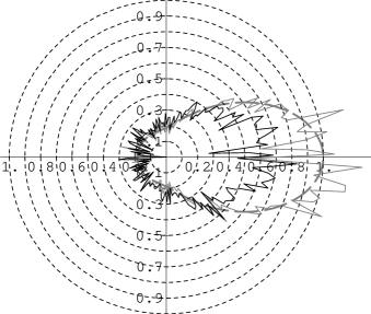
Chapter 7 Experimental Verification
Die gefährlichste Weltanschauung ist die Weltanschaung derjenigen, die die Welt nicht angeschaut haben.
THE experimental verification of the derived theoretical models of chapters 4 and 5 is hampered by the fact that it is nearly impossible to design a measurement setup that allows a sufficiently good definition of the -rays interaction depth. The same statement holds for the evaluation of the detector performance concerning the energy resolution, spatial resolution and depth of interaction resolution. For a -ray impinging normally to the plane of the photodetector’s sensitive area, the depth at which the photon interacts is subjected to a random process and it is not accessible by experimental preparation. The possibility of using a sandwich-like configuration consisting of several inactive layers and only one scintillation layer, but all having the same optical properties, has been discarded for economic reasons. Moreover, it is questionable if these set of sandwiches really reproduce the properties of a single thick scintillator slab. Lateral irradiation with a collimated -ray, as was explained by Moses and Derenzo [Moses:1994] or Huber et al. [Huber:1999] for the use with small scintillation crystal needles, has to be discarded for another reason: due to the large transverse spatial extension of the crystal slab, the intensity of the -ray would decrease quickly from the edge and lead to very high counting statistics at the side of the detector that faces the radioactive source and very low statistics at the opposite side.
Another important problem is caused by the collimation of the -ray beam. When using collimators, one has to keep in mind that, for the energy of the annihilation photons, the probability for scattering is already rather high. For lead or tungsten, which are the most suitable materials for collimators, the photon cross-sections for photoelectric absorption and incoherent Compton scattering actually have very similar values. This leads to a high fraction of Compton scattered photons in the -ray beam and fans out the collimated beam. A second possibility is given by electronic collimation using a second coincidence detector, which is required anyway for Positron Emission Tomography. In this case, the spatial extension of the radioactive source has to be taken into account. Commercially available positron emitters normally have a diameter of one millimeter or more. Modern -ray imaging detectors already reach intrinsic spatial resolutions in the range of to a few (Correia et al. [Correia:1999], Joung et al. [Joung:2002] and Tavernier et al. [Tavernier:2005]) and one has to correct the obtained results for the spatial extension of the -ray source. The same arguments hold for beams collimated with a tungsten or lead collimator.
In this section a method is explained, detailing how information about the depth of interaction can be obtained without the necessity of preparing several experiments for different DOIs. This method is subsequently used to verify the analytic model for the signal distribution derived in chapter 4. Also, the four first-order moments, namely , , and (refer to chapter 5), are measured at 81 uniformly distributed test positions within the sensitive area of the photodetector.
7.1 Experimental Setup
For the measurement of the moments, two identical and opposite -ray detectors were used. Each module consisted of a single large-sized scintillator-block with spatial dimensions . As scintillation material, cerium-doped lutetium oxyorthosilicate (, also LSO, invented by Melcher and Schweitzer, [Melcher:1992]) was chosen for the excellent matching of its properties with the requirements for Positron Emission Tomography (cf. section 3.2.1). According to the arguments given in section 4.1 and the findings of section 4.2, the five side-surfaces that were not coupled to the photodetector, had to be covered with a highly anti-reflective layer. Furthermore, these sides were not polished but only fine ground. The reason for this decision was not only economical. A polished crystal surface together with the glue of the painting or the epoxy possibly builds an interface of two optical media with different refractive indices. Most probably, this would lead to total reflections because the refraction index of LSO is, at 1.82, rather high. Black epoxy resins can be used to realize high quality anti-reflective coatings that generally out-perform most other resin types in terms of mechanical properties and resistance to environmental degradation. We also observed that the reflections caused by simply black painted side-surfaces result in a high fraction of reflected scintillation light that renders the determination of the distribution’s second moment with the method presented here almost impossible.
electronics PSPMT optical grease scintillator
As position sensitive photodetector, the Flat-Panel type multi-anode PMT H8500 from Hamamatsu Photonics K.K. [data:H8500] was chosen. Photomultipliers generally have outstanding signal characteristics, namely very high gains together with low noise, fast response, high stability and a long life. The price per unit sensitive area is also very low compared to other photodetectors making it a very versatile light detector. The H8500 is characterized by a sensitive area with a dimensional outline of only . That is to say, it is an extremely compact PMT with a very low dead area at the borders, allowing a high packing density and very compact -ray imaging detectors. The small thickness of the H8500 indicates that the 12-stage metal channel dynode system is also very compact, leading to a low electron transit time and electron transit time spread. The H8500 has a borosilicate window of refractive index at incident wavelength and a thickness of . It has a standard bi-alkali photocathode of thickness Å [hamamatsu:privcom] with a complex refractive index of (Motta and Schönert [Motta:2005]). The anode consists of an array of segments of size and an inter-segment pitch of .
A non-curing optical grease (Rhodorsil Pâte 7, Rhodia Siliconi Italia) was used to attach the LSO crystal to the entrance window of the H8500. The refractive index of this gel () lies in between the refractive indices of the scintillator and the entrance window. It avoids air-gaps between the two media and optimizes the scintillation light collection. Figure 7.1 shows schematically the internal configuration of the detector module.
The electronics contained in each detector module includes the proportional resistor network displayed in figure 5.8 of section 5.4.1 together with the summation amplifier (figures D.1 and figures 5.11(a), 5.11(c) of section 5.4.1), the high-voltage power supply (Hamamatsu, [data:C4900]) and the preamplifiers and line drivers displayed in figures D.2 and D.3. of Appendix D. The preamplifier and line-driver modules perform the current-to-voltage conversion, restore the baseline of the signal and amplify it for an optimal matching of the input voltage range with the analog-to-digital converter module. The basic configuration from Siegel et al. ([Siegel:1996]) was adopted for the 2D proportional resistance network and the values , , and were taken for the summation resistors (refer to section 5.6.2).
Although the method for depth of interaction detection presented in this work is not confined to imaging modalities based on coincidence detection, the experiments have to be carried out in temporal coincidence for two reasons. First, approximately of the natural lutetium contained in LSO is radioactive (, years) causing a background of roughly 280 detected single events per second and of scintillation material. decays via -decay with a maximum energy of and with subsequent decays of the and levels of through -decay with transition energies of , , and (Lauckner et al. [Lauckner:2001], Melcher and Schweitzer [Melcher:1992], Huber et al. [Huber:2002]). Therefore, a -ray source of high activity is required for the use of LSO with single photon imaging modalities, whereas the isotope produces only a negligible background event rate in temporal coincidence mode. A second important advantage of coincidence detection is that the -ray beam can be collimated electronically as long as the coincidence detector is also sensitive to the -ray’s impact position. Such a collimation should be preferred for the reasons explained above and because it allows simple off-line manipulation of the data set as well as a variation of the collimation diameter.
The electronic configuration of the generation of the coincidence trigger and the data-acquisition system is shown in figure 7.2. For the derivation of the trigger impulse one preferably uses the additional last dynode signal provided by the H8500 PSPMT. The signal from the last dynode is synchronous to those from the anodes and its pulse height is proportional to the total amount of detected scintillation light. Therefore, we can use this signal instead of a fraction of the anode-signals for energy discrimination and detection of temporally coincident events. Two channels of the octal leading edge discriminator 623B from LeCroy were used to establish the low energy threshold for both dynode signals. The sum of the width of both resulting logic pulses defines the time coincidence window which was set to its lower limit of approximately , i.e. using the minimum pulse width of provided by each discriminator module. These signals are fed directly into a logic unit (Ortec CO4020) configured for coincidence mode operation. From this signal two pulses are generated. The first pulse has a duration of and is delayed by . This signal is used for triggering the 12-channel charge integrating analog-to-digital converter module (Zavarzin and Earle, [Zavarzin:1999]). Each of the 12 channels is internally equipped with a delay line, baseline restoration, signal shaping and an analogue integrator whose integration time is defined by the width of the trigger pulse. The internal delay of the input signals by comes in very handy for the derivation of the coincidence trigger. The second pulse of width from the logic unit and without delay is fed into the common veto input of the discriminator unit in order to avoid re-triggering of the ADC module while a conversion is in progress. Once the digital data is available, it is transfered to a PC using a 100MB Ethernet connection.
The complete experimental setup was mounted inside a black room in order to minimize detection of stray light (refer to figure 7.3). While the coincidence module was mounted stationary, the test detector was mounted on top of a - translation stage with a precision of and driven by PC-controlled stepper motors. A source of nominal activity was aligned with the center of the coincidence detector. Furthermore, it was placed at the large distance from this detector but as close as possible to the test detector (distance ). Due to geometric arguments, the positions of valid annihilation events detected at the test detector have to lie within a small circular spot of diameter whenever they are detected at the coincidence detector within the circle of diameter . In the experiment, was set to approximately .
After the alignment of the radioactive source and both modules, the test detector was calibrated for offsets introduced by the preamplifier and the analogue-to-digital converters. For this purpose, the charge integrating digitizing card provides an internal clock allowing a fast simultaneous offset measurement of all 12 electronic channels with the high voltage of the Photomultiplier tubes turned off. The gain of the different electronic channels was supposed to be nearly the same and was not calibrated.
The energy, both centroids and the second moment of the signal distributions of valid coincidence events were measured at 81 different positions . With the aid of the translational stage, the test-detector was automatically moved to each of these positions as indicated in figure 7.4 and 192000 coincidence events were registered before moving to the next position. The data was stored in raw format (all 12 electronic channels for each event) for subsequent processing, i.e. computation of the moments, electronic collimation and energy and position filtering. Approximately of all events produced an ADC overflow or underflow. These events have been removed from the data sets.
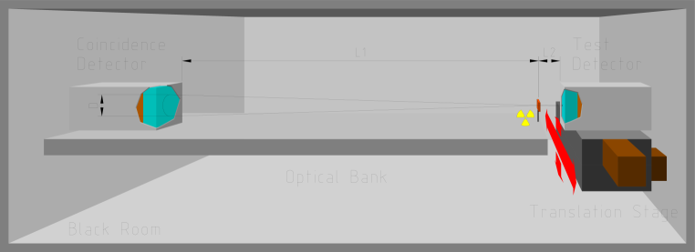
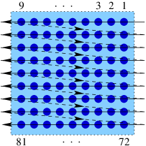
7.1.1 Spatial Extension of the Radioactive Test-Source
A point source of nominal activity was used for these measurements. The radioactive isotope is absorbed in an ion-exchange bead and fixed at the geometric center of an epoxy resin capsule. However, this source with a diameter of cannot be considered as a point-like source for the present experiment, since the spatial resolution is expected to be of the same order and therefore one has to correct the results for this finite size effect. Furthermore, one has to take into account that the source is a -emitter and that the positrons have a finite range before giving rise to the annihilation radiation (refer to section 3.3.3). This leads to a penetration of -particles into the epoxy resin and also to an expected higher activity at the center of the source pellet. The resulting effective source diameter can hardly be measured and a description with analytic models would be too cumbersome. Instead, it was estimated using Monte Carlo simulations (Sanchez, [sanchez:privcom]) with GEANT 3 (Brun and Carminati [Geant3:1994]).
Figure 7.5(a) shows a normalized density plot of the positron endpoint positions of simulated events projected onto the --plane. However, for the estimation of the effective diameter only the radius is of interest. One has to normalize the bin-content of the histogram for with because the circumference and therefore the counts in each bin grow with the radius. The simulation results are displayed in figure 7.5(b). In order to compute the FWHM from the histograms of the radii, the following empirical model distribution
| (7.1) |
was least-square fitted to the data (figure 7.5(b)). The obtained best-fit parameters are:
| (7.2) |
Equation 7.1 can be easily inverted for finding the FWHM of the distribution:
| (7.3) |
and leads to the final result for the effective source diameter
| (7.4) |
7.1.2 Model Distribution for Event Statistics
As mentioned in the introduction of this chapter, another experimental difficulty in the setup is imposed by the fact that one cannot easily prepare a measurement for the distribution moments at well defined interaction depths. Unfortunately, one is only able to define the impact position along the two spatial directions that are normal to the -ray beam. The position of interaction along the remaining direction parallel to the beam is subjected to the random processes of photoabsorption and Compton scattering. For thick scintillation crystals one therefore faces a large uncertainty in this third position component while thinner crystals produce a lower uncertainty. However, the attempt to reduce the crystal thickness would lead to lower interaction probability (efficiency) and would clearly change the optical behavior of the crystal.
Another possibility consists of properly defining the depth of interaction and one of the spatial dimensions or . This can be achieved experimentally when a -ray beam parallel either to the -axis or the -axis enters the crystal at one of the small sides normal to the sensitive area. The remaining component of the impact position can be measured sufficiently well by means of the center of gravity algorithm, since no superposition from different depths occurs. An important drawback of this method is the attenuation of the -ray beam along the indeterminate spatial direction. Especially for large-sized crystals this leads to low statistics at the side opposite to the -ray source. Furthermore, it does not allow fast and handy calibrations of the detector.
The depth enhanced charge dividing circuits presented in chapter 5 allow for a more suitable approach since all three spatial components of the impact position can be measured simultaneously, provided that the spatial resolution is sufficiently good and the dependency of the second moment on the depth of interaction is known and sufficiently pronounced. In this case, one expects a characteristic distribution of the second moment which has to be a superposition of the detector response at all possible interaction depths. By making the following assumptions, an adequate model for the distribution of the second moment was derived. First, it is supposed that there is a constant intrinsic resolution for the spatial direction parallel to the -ray beam. This is clearly only an approximation since there are various possible effects that can make this intrinsic resolution depend on the position. However, the superposition requires integration over the crystal’s spatial extension along -axis and, therefore, does not admit very sophisticated integrands. Furthermore, the detector’s response function for an exactly defined depth of interaction is expected to have Gaussian shape and width . The second assumption is that the second moment at all points depends linearly on the depth of interaction. This allows for linear transformations of the integration variable and legitimates the use of the model for the second moment instead of the true depth of interaction. Evidence for this second assumption has been reported by Antich et al. [Antich:2002] and was also predicted by the model derived in chapter 4 (refer to figures 4.10(a)-4.10(d) in section 4.2).
The -ray beam’s intensity decreases exponentially due to the attenuation within the crystal. Therefore, the amplitudes of the Gaussians decrease with increasing depth of interaction and one obtains the convolution
| (7.5) |
where is the attenuation coefficient of the scintillation crystal for the -ray energy of interest, and and are the upper and lower limits of the crystal respectively. Outside of these limits one does not expect any events and the distribution is equal to zero. The subscript indicates that all parameters in equation 7.5 are understood to refer to the moment space. Figure 7.6(a) illustrates the integral in equation 7.5. An explicit form is obtained by resolving the previous integral:
| (7.6) |
where stands for the error function. Since there is a linear dependence between the second moment and the depth of interaction, the corresponding intrinsic depth resolution in the position space is given by scaling . The integration limits and in equation 7.5 define with a measure for the true crystal thickness in the moment space. Therefore, in position space one obtains the resolution
| (7.7) |
In figures 7.6(c) - 7.6(e), plots of the model distribution for different parameters are shown. One can observe that the distribution adopts a Gaussian shape for the case . Actually, it can be seen directly from the definition 7.5 that the distribution approaches a Gaussian-like shape in the limit . If is large compared to and , the distribution approaches an exponential decay distribution that is horizontally shifted by . For both these limits, fits with this special model distribution cannot produce reliable estimates for the parameters and . Clearly, these limits have to be avoided with a proper experimental setup. In the experiment, the majority of histograms did not approach these limits and the fit routine gave acceptable results.
Note that all assumptions that were made for the derivation of the model also hold for the zeroth moment, i.e. the energy, and both first moments (the centroids). As shown in section 5.8, these moments also exhibit depth of interaction dependence. In particular, near the crystal borders it shows the characteristic shape displayed in the examples in figures 7.6(a)-7.6(e) and, therefore, has to be preferred to the Gaussian model. The model (7.6) was modified in some cases by adding a constant or linear background.
Figures 7.7(a)-7.7(f) show some examples of the model fitted to distributions measured with the experimental setup that was described above. The left column shows best fits for the case when the -ray beam entered the detector at the center of the PSPMTs sensitive area (). The right column shows the results obtained when locating the beam at one of the corner positions, e.g. . It can be seen that the model reproduces well the measured distributions for both cases. All other positions will result in distributions of a form in between these two extreme cases.
A more reliable method to estimate the goodness of the fit results is given in Press et al. [Press:1992] and is reasoned as follows. The probability that a value for obtained by fitting the model to experimental data occurs for a determinate number of degrees of freedom is given by
| (7.8) |
where is the Euler gamma function and is the incomplete gamma function. The values of , and are given together with the graphs in figures 7.7(a)-7.7(f). Note that in this estimation nothing is known about the achieved precision of the best fit parameters. It is possible to obtain good values for and while the errors of the adjusted parameters could be rather large. Actually, this is the case when the measured distributions becomes similar to the Gaussian or exponential case. These limits contain only poor information on , and and, thus, their errors are quite large.
7.2 Results
First of all, the method of depth of interaction determination is tested using an inclined -ray beam. This inclination must be reflected somehow in the histograms for the second moment and the centroids. Likewise, the broken symmetry of the light distribution that was explained in section 5.8.3 must become apparent from the same histograms if the -ray interacts with the crystal near one of its absorbing borders. Once this has been tested, it will be shown that the quality of the second moment is sufficiently good in order to filter subsets with similar DOI parameters out of the data.
After these qualitative crosschecks, the moments measured at the 81 test positions were compared to the predictions of the model for the signal distribution established in chapter 4. In addition, the possible resolution which can be obtained for each of the lower-order moments is measured.
7.2.1 Qualitative Verification of the Method
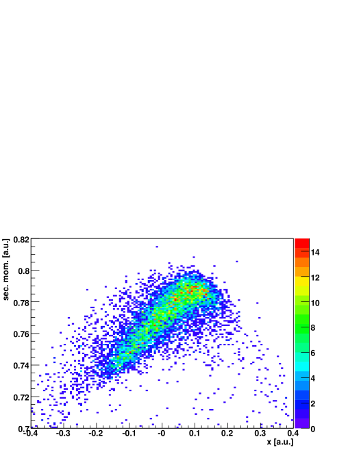
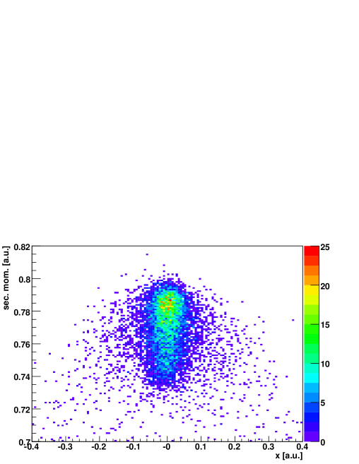
In order to crosscheck the presented method, the test detector was irradiated with an electronically collimated -ray beam inclined by with respect to the -axis. The beam was adjusted in such a way that its axis crossed the geometric center of the crystal and laid in the --plane. In figure 7.8(a), is plotted versus the -centroid and a correlation between these two measures is apparent. In contrast to this, one cannot observe this correlation for the -centroid (figure 7.8(b)) since the -ray beam is perpendicular to this direction. Antich et al. [Antich:2002] already reported this result. They studied the possibility of using crossed-wire photomultiplier tubes together with large-sized scintillator crystals for three-dimensional position readout for SPECT/PET. However, they needed to digitize all 32 channels from the Hamamatsu R2486 PSPMT in order to obtain this impact parameter. Using the enhanced charge dividing circuits described in chapter 5, only 5 electronic channels were necessary and the moments were computed analogically and online.
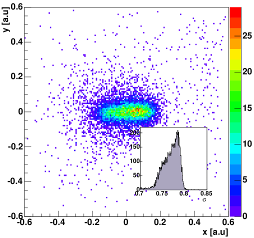
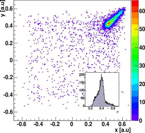
The distribution of the measured centroids within the --plane is shown in the density plot 7.9(a). There is an apparent blurring along the -direction and almost none along the -direction. The small inset shows the histogram for the standard deviation of the signal distribution. In the same figure to the right, the distribution for the - and -centroids is shown for a -ray beam hitting the test detector at an outer corner of the photocathode. The blurring of both centroids is now caused by the effect described in section 5.8.3 and not by the -ray beam itself, because this time it is normal to the photocathode. The small inset shows the corresponding distribution of the second moment. Note that due to mechanical limitations of the experimental setup, the radioactive source could not be placed very close to the detector when the detector was inclined by . Therefore, a more important blurring in all directions is observed in figure 7.9(a).
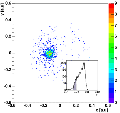
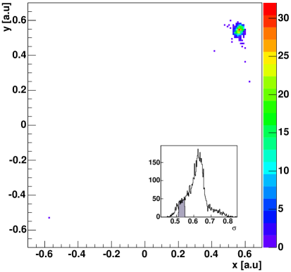
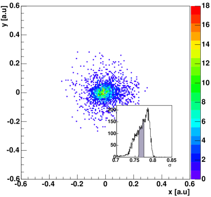
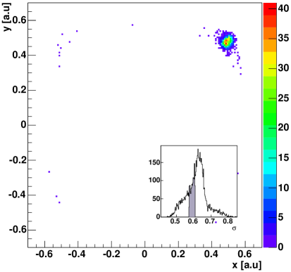
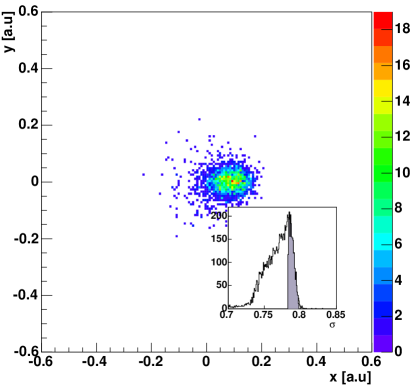
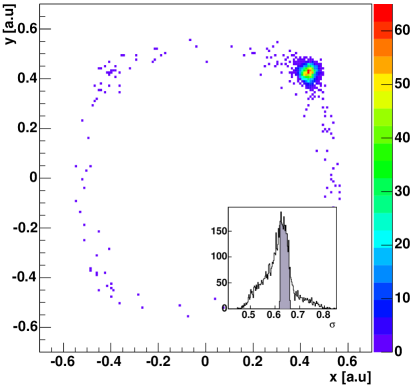
The information that is given for each detected event with the second moment (or alternatively the standard deviation) can be used for filtering out events with a specific second moment. This is illustrated in figures 7.10(a)-7.10(f). In the left column, three density plots for the - and -centroids are displayed. The shaded regions of the histograms in the small insets indicate those events that are selected for display in large density plots. This was repeated for three characteristic subsets of -values (low, medium and high). By this means, the long spot in figure 7.9(a) could be fragmented into three smaller spots of almost circular shape. The same procedure was repeated for the normal -ray beam impinging on an outer corner of the photocathode. Once again, a clear discrimination of subsets of similar - and -centroids is possible. All observed effects in these preliminary experiments can be easily explained assuming that:
-
1.
the signal distribution behaves like the analytic model derived in chapter 4,
-
2.
the enhanced charge divider circuit presented in chapter 5 measures indeed the second moment, and
-
3.
the arguments given for deriving the fit model (expression 7.6) in fact describe the steps of the formation of this distribution.
Throughout the rest of the present work it is therefore assumed that the second moment (or alternatively the standard deviation) is appropriate for estimating the depth of interaction.
7.2.2 Validity of the Model for the Signal Distribution
In order to test the accuracy of the analytic model for the signal distribution, some further effects have to be taken into account. The model includes the most important physical effects until the scintillation light is absorbed, with or without its detection. In addition, the photomultiplier is assumed to behave as ideal. That is, neither photoemission from the dynode-system, nor reflections inside the PSPMT, nor effects like dark-current are considered. Actually, photomultipliers behave almost ideally in many aspects.
After the photoemission of an electron, it is attracted by the strong electric potential of the first dynode where its impact causes various secondary electrons. In the case of the H8500 from Hamamatsu, this process is repeated twelve times because it has twelve dynode stages. The special design of these dynodes provides for low transverse dispersion of the electron avalanches. These are finally collected by the anode pads. The size and pitch of the anode pixels are found to be and respectively [data:H8500]. However, the effective sensitive area of the device () is larger than or . This is because the electron avalanches can be focused towards the anode pads and the small gaps between them are not critical. Dividing the effective area by the total number of pixels, one can define the effective pixel size , area and pitch to be , and , respectively.
The particular combination of photocathode, focusing dynodes and anode matrix configuration performs an integration by intervals of the scintillation light. The intervals are defined by the effective pixel size and its position. The integration gives a set of 64 positive numbers that correspond to the amounts of scintillation light detected at each of the 64 equal-sized segments of the photocathode. It was already mentioned that the light sensitivity can vary significantly from one anode segment to another. The typical value for this uniformity is given by the manufacturer and is of the order of 1:3. Eventually ratios as high as 1:6 can be reached. Therefore, an anode uniformity map is provided with each delivered PSPMT. In order to obtain reasonable predictions of the detector energy response behavior, one has to multiply each of the 64 values obtained by integration with the relative anode sensitivity of the segment that corresponds to this integration interval.
From this set of corrected numbers, the moments can now be computed. The energy is obtained by simply summing up all 64 corrected numbers. For computing the centroids and the second moment, the numbers have to be multiplied with linear and quadratic weights respectively before building the sum. Since it was shown there that all configurations of charge dividers can be configured to reproduce an exact linear weighting along both transverse directions, the weights for the centroids (normalized first order moments) are nothing but the center positions of the anode segments. The situation for the second moment is more complex due to several reasons. First of all, one has to decide which type of second moment is appropriate. By definition (5.7), many second moments are possible in the multivariate case, e.g. , , etc.. Due to limitation by electronic design, minimum cost requirements and the desire to maximize the SNR of the measured moment, the composite second moment is chosen. In the ideal case, the weights would then be given by the sum of squares of the anode center positions: . However, this behavior can only be approximated with the charge divider configuration that uses proportional resistor chains. Therefore, higher orders and mixed terms of the center position also occur. Furthermore, the electronic signals have to be amplified and prepared for integration, introducing corrections that would be far too complex to be treated analytically. For these reasons, the impulse response of the circuitry for the second moment computation for each of the 64 segments was simulated using the circuit simulation program Spice. The response was fitted using a polynomial Ansatz consisting of even orders of and as well as their mixed contributions, and with the following result:
| (7.9) |
All mathematical operations performed by the PSPMT as part of the present -ray imaging detector can now be written in the form
| (7.10) | |||
| (7.11) | |||
| (7.12) | |||
| (7.13) |
The values for all parameters of the signal distribution together with the configuration of the enhanced charge divider circuit was described in section 7.1. The electronic amplifier configuration is sketched in appendix D. Figures 7.11(a)-7.11(d) graphically represent the weights for the centroids, the second moment and the anode uniformity.
The moments were then computed numerically for the 81 different transverse positions , with and at the two limit values for the depth of interaction and . The data obtained from the measurement of the different moments at these positions are, however, distributions of all possible values of between these two limits. One can obtain these limits (parameters and ) from the experimental data by means of the fit model (expression 7.6) described in section 7.1.2.
In order to compare the parameters and to the computed moments for the limits and one has to take into account that the analog-to-digital conversion introduces a global and linear shift of the measured moments which is very difficult to predict analytically. The ADC module internally shapes, delays and integrates the current pulses fed into their inputs before the analog-to-digital converter maps the area to an integer of the interval ( and are reserved for under- and overflows, respectively). This sequence of transformations produces both a global offset and a global proportionality constant . The determination of these parameters is best done by minimizing the sum of differences since the measurements are subjected to statistical errors. Hence, the following sum is defined:
| (7.14) |
Here, stands for one of the four moments , , and , each having its own pair of transformation parameters and . That is, the sum in equation (7.14) has to be computed four times. The optimum values for and of each moment are given by those that minimize . Table 7.1 summarizes the results for a signal model without diffuse reflected background light and another including the latter contribution.
In figures 7.12(a)-7.13(h), the measured and predicted values are displayed for a model that includes the reflective background discussed in section 4.1.6. For clarity, the predicted values (gray dashed line) are displayed in 2D-plots together with the measured data (black data points) and in the order illustrated in figure 7.4. The right column of plots shows the deviation between the model prediction and the measured values (light-gray solid lines), displayed together with the measurement errors (dashed black lines).
An important observation is that the model distribution derived in chapter 4 reproduces very well the spatial dependence of the three non-trivial moments. In the case of the zeroth moment, i.e. the energy, the agreement was, however, poorer. The model fails to reproduce correctly the details of the energy variation over the sensitive area especially for the upper limit in the interaction distance (). Note that this affects the non-trivial moments only marginally because the aim of normalization is to suppress the dependency on the trivial moment. The measured centroids (figures 7.12(a)-7.12(h)) exhibit errors at the central positions that are much larger than the discrepancy between prediction and measurement. Most likely this is caused by the fact that the parameters and cannot be estimated very well with the fit model (7.6) when the distribution are nearly of Gaussian shape. In the case of the composite second moment (figures 7.13(a)-7.13(d)), it is observed that the agreement between model and measurement is much better in the limit (parameter ) than in the limit (parameter ). Since this also occurs for the zero-order moment (figures 7.13(e)-7.13(h)), it has to be assumed that the model for the background light does not reproduce well the distribution of the additional light. However, a model with the background light switched off, fails completely to predict the trivial moment (figures 7.14(a)- 7.14(d)). Therefore, a detailed study of the reflection properties is necessary in order to find a more reasonable background model.
Other reasons for the remaining deviations between measurements and those obtained from the theoretical model are Compton scattering as described in chapter 6, lack of mechanical precision and possible light reflections inside the PSPMT, e.g. at the dynode system and the housing. In particular, the mechanical tolerance may be of relevance. While the precision of the motorized translation stage used () is sufficiently good for our purposes, the remaining parts of the mechanical setup like housing, source holder and test detector mounting, not only miss this precision but are estimated to introduce errors in the transverse directions up to . This precision has to be significantly increased if a model with higher accuracy is required. Table 7.2 summarizes some statistic estimators of all observed measurement errors and deviations between model (with residual reflections) and measurement. Except for the centroids, relative errors are used. Absolute errors have been preferred for the centroids because at nominal positions around , the relative error of the centroid will diverge even for very small absolute errors. All relative errors are of the order of 10%, while the absolute errors of the centroid are about . Note that this corresponds to the estimated mechanical uncertainty of the test detector assembly.
| moment | p. | model-measure deviation | measurement error | unit | ||||||||
|---|---|---|---|---|---|---|---|---|---|---|---|---|
|
|
|||||||||||
|
|
% | ||||||||||
|
|
% | ||||||||||
|
|
mm | ||||||||||
|
|
mm | ||||||||||
|
|
mm | ||||||||||
|
|
mm | ||||||||||
|
|
% | ||||||||||
|
|
% |
For the case of a model without diffuse reflections, only the results for the zeroth order moment have been plotted (figure 7.14(d)). The results for the other moments are very similar to the case with reflected background and their errors of the same order. Actually, this model was only applied to demonstrate that even for very low reflectanceivity of the absorbing coatings, residual reflections on these surfaces cannot be neglected if the model is also required to yield good agreement for the trivial moment.
7.2.3 Moments as 3D Position Estimate
At the end of this chapter, an estimation is given of what 3D-spatial resolution can be expected from the presented detector setup if the raw moments were used as position estimates. While it has been reported elsewhere (Clancy et al. [Clancy:1997], Joung et al. [Joung:2002], Tavernier et al. [Tavernier:2005]) that this is not satisfactory for many reasons, the results are given here not only for completeness. Instead, the availability of an analogically computed second moment that can be used to estimate the depth of interaction via the standard deviation is an interesting extension of the conventional Anger logic. Unfortunately, this new estimate suffers from the same problems as the centroids: as the -ray’s impact position gets closer to one of the borders, the light distribution is distorted and the moment is subjected to an additional variation not caused by the interaction depth. The following chapter will treat this problem by presenting an algorithm for recovering the true three-dimensional impact position from the set of moments.
In order to obtain the standard deviation from the three non-trivial and normalized moments , and , the definition of the variance for two dimensions can be applied only with some modifications:
| (7.15) |
where denotes the expectation value of . Note that is just the additional moment provided by the enhanced charge divider. and are the centroids and , respectively. However, one has to take into account that different electronic amplifier designs (refer to Appendix D) are used for the centroids and for the composite second moment. Therefore, they arrive with different gain-factors at the ADC-module. Moreover, as it was discussed before in this section and also in section 5.4, proportional resistor chains do not provide exactly the second moment, but also include higher than quadratic orders. We define, therefore, the ID-estimator as the square root of the composite second moment , reduced by the transverse dependency defined in equation (7.9):
| (7.16) |
For measuring the three-dimensional resolution of the detector, model (7.6) is fitted to the histograms of the centroids and the energy for all 81 test positions. The FWHM is computed from the best fit curves and its error is estimated by applying standard error propagation. Equation (7.7) with the corresponding error propagation was used for the bare second moment and . Since the centroids always reproduce a compressed image of the radioactive sources, they have to be expanded by applying the inverse of the position-to-centroid mapping. However, not only the center-position is shifted in this way but the point-spread function is also proportionally blurred. This expansion has to be applied to the FWHMs of the centroid distributions and the FWHMs also have to be corrected for the finite source diameter (7.4). The results are displayed in figures 7.15(a)-7.16(d). As expected, the energy and centroid resolutions degrade considerably towards the edges and borders of the crystal. The values for and likewise depend strongly on the transverse coordinates. Nevertheless, a good depth of interaction estimate is given by , reaching a mean DOI resolution of and its best value of at the center. This a high resolution in comparison with the methods discussed in section 3.4.1. The resolution of the bare second moment becomes very poor at certain test positions. These positions are part of a connected region of the PSPMT’s sensitive area, at which the resolution of this moment is subjected to strong variations. This effect can be easily explained by the fact that the parabolas of the bare second moments for different DOIs intersect at this particular region. As a consequence, even large variations of the interaction depth lead only to very small variation for this moment, although the intrinsic width of the point-spread function for the DOI remains the same. Then, the denominator of equation (7.7) becomes very small and this explains the observed large values (see also Lerche et al. [Lerche:2005b]).
Mean values, standard deviations, maximum and minimum values for the resolutions of the five moments are summarized in table 7.3.
| Moment | Mean | StdDev | Min | Max | Unit |
|---|---|---|---|---|---|
| 24.9 | 8.8 | 16.6 | 71.2 | % | |
| 3.4 | 3.2 | 1.4 | 20.9 | mm | |
| 3.3 | 3.1 | 1.3 | 19.9 | mm | |
| 15.9 | 23 | 2.2 | 73.1 | mm | |
| 4.9 | 1.8 | 1.9 | 9.0 | mm |
Chapter 8 3D-Impact Position Reconstruction
Imagination is the real and eternal world of which this vegetable universe is but a faint shadow.
AS mentioned in chapter 2, the reason for using large-sized continuous scintillation crystals111In the sense of section 4.1. is mainly founded in the aim to reduce the cost of -ray imaging detectors. Clearly this can only be justified if there is no significant loss in the performance of the different characterizing parameters. With the development of the block detector by Nutt and Casey [Casey:1986], a promising technique for building PET scanners appeared. Since the intrinsic spatial resolution of the -ray imaging detector can be obtained by selecting an adequate size of the crystal element, this design has been adopted by several research groups for use with small animal positron emission tomography. There have been some alternative efforts to use continuous crystals for -ray imaging for coincidence and single photon imaging (Siegel et al. [Siegel:1995] and Seidel et al. [Seidel:1996]), relying on the Center of Gravity algorithm implemented as described in section 5.2. They report strong edge artefacts, especially when thick crystals for the detection of high energy photons are required. As shown in section 5.8, these errors are inherent in the CoG algorithm for crystals of finite size and thickness. Other groups abandoned the conventional Anger positioning scheme in favor of statistic based positioning (Joung et al. [Joung:2002]) or the use of neural networks (Tavernier et al. [Tavernier:2005]), but at the expense of independently digitizing all photodetector segments. Despite the fact that a better spatial resolution can be achieved by using these methods, they are obtained by drastically increasing the number of electronic channels. Due to the fact that the data acquisition and analysis system has to be more complex, the final cost of the device is significantly increased.
8.1 The Truncated Moment Problem
In chapter 5, DOI enhanced designs of charge dividing networks were presented. These networks have been developed primarily in order to allow for an efficient estimation of the depth of interaction of the -ray. However, the experimental results of chapter 7 revealed that using the standard deviation as DOI estimator yields a good resolution at the central region of the sensitive area but degrades towards the crystal edges. The reason for this effect is that near the edges, the detected signal distribution is distorted because a large fraction of the scintillation light is absorbed by the black painted surfaces. This causes a change in all moments and their use as three-dimensional position and energy estimators becomes a poor approximation for a large fraction of the sensitive area.
Using directly the second moment instead of the square root of the central second moment (i.e. the standard deviation) is not possible without problems because it is subjected to strong quadratic variations along the transverse spatial directions. Moreover, the second moments for different DOI intersect at an annular region of the sensitive area. That is, there is a region of the sensitive area where the measured second moments of events with different depth but same --position are almost equal to each other. For points within this region, no DOI information can be obtained directly from the second moment since all DOIs are mapped to a similar value. However, this applies only to the non-centered second moment. For the standard deviation no intersections are observed (refer to chapter 7 and also Lerche et al. [Lerche:2005b]).
As a consequence, one is tempted to recover the true impact positions from the available moments given by equations (7.10)-(7.13). This is a typical inverse problem and for its solution one needs to find the following three functions, or at least good approximations for them.
| (8.1) | |||
| (8.2) | |||
| (8.3) |
No inverse function is required for the energy since is used for normalization of the moments involved and the true energy of the detected event, i.e. the amplitude of the signal distribution 4.26, acts as a multiplicative constant.
A special feature of the present inverse problem is that one has to reconstruct distribution parameters from some known moments of the distribution. Thus, it is very similar to the truncated moment problem (Kreĭn and Nudel’man [Krein], Tkachenko et al. [Tkachenko:1996]). There are three essentially different types of moment problems depending on which type of intervals they are defined on. For historical reasons, the moment problem on the semi-infinite interval is called the Stieltjes moment problem. On it is called the Hamburger moment problem and on the bounded interval it is referred to as the Hausdorff moment problem.
8.2 Polynomial Interpolation
A promising technique for inverting the system of equations (7.10)-(7.13) is given with standard polynomial interpolation. The approximation of functions by interpolation embraces a large variety of methods including Spline interpolation, Taylor series, continued fractions, etc., which are well understood and widely used (see for instance Kincaid and Cheney [Kincaid] and Press et al. [Press:1992]).
Polynomial interpolation has been recently applied to a rather similar problem (Olcott et al. [Olcott:2005], [Olcott:privcom]). They studied the spatial response of a scintillation crystal array coupled to a position-sensitive avalanche photodiode (PSAPD). These photodetecting devices present a promising technology for -ray imaging detectors but suffer from a strong pincushion-like distortion. Olcott et al. used finite element methods for solving Laplace’s equation on the resistive layer of the PSAPD in order to predict its spatial response function. Finally, they expanded the supposed detected positions using a two-dimensional polynomial basis, thereby obtaining a matrix of coefficients that could be inverted and applied for linearity correction with encouraging results.
The differences compared to the inverse problem posed by equations (7.10)-(7.13) and the detector setup discussed in the present work are minor. Instead, the fact that an additional measure of the distribution, i.e. the second moment, is made available, probably increases the performance of the method.
8.2.1 Polynomial Interpolation in One Dimension
Before applying this method to the inverse problem, some useful properties are summarized (refer to Kincaid and Cheney [Kincaid]). The interpolation problem consists in finding a polynomial of lowest possible degree for a given set of known data points . If the interpolation points are distinct real numbers, then there is a unique polynomial of degree at most such that
| (8.4) |
This theorem holds for arbitrary values and a proof can be found in Kincaid and Cheney [Kincaid]. The interpolation polynomial can be written in terms of powers of
| (8.5) |
which, together with the interpolation conditions (8.4), leads to a system of linear equations that can be used for determining the coefficients . This system has the following form:
| (8.6) |
The coefficient matrix is known as the Vandermonde Matrix (also called an alternant matrix), and has the form
| (8.7) |
While the Vandermonde matrix is non-singular because the system has an unique solution for any choice of , it is often ill-conditioned and does not allow an accurate determination of the coefficients . There are still other algorithms for polynomial interpolation that all produce the same result, since the solution is unique as stated above. Depending on the posed problem, they have advantages and disadvantages. The amount of work involved to obtain in equation (8.5) seems excessive and algorithms that intrinsically implement Horner’s scheme222Horner’s scheme rearranges a polynomial into the recursive form and therefore requires only additions and multiplications for evaluating the polynomial. may be preferred. However, as will be shown later, the expansion into the polynomial never has to be computed because there is no need to know the functional form of the distribution. Only the three-dimensional impact position has to be estimated.
The discrepancy between the true function that produced the data points and the interpolating polynomial at the position is given by . This error can be expressed as a function of the ()th derivative of at the corresponding position as follows:
| (8.8) |
where it is supposed that all distinct interpolation nodes lie in the interval , and that to each in this interval corresponds a point in that satisfies equation (8.8). The error of the polynomial can be optimized by choosing adequate interpolation nodes. When the roots of the Chebyshev polynomials defined by
| (8.9) |
on the interval are used as nodes, equation (8.8) transforms into
| (8.10) |
The roots of the Chebyshev polynomials are given by the following closed-form expression:
| (8.11) |
Again, proofs for both error estimates (8.8) and (8.10) can be found in Kincaid and Cheney [Kincaid].
8.2.2 Polynomial Interpolation in Higher Dimensions
For clarity, higher dimensional interpolation is explained considering the two-dimensional case. Generalizations to higher dimensions are straightforward using the results derived in this paragraph. In the two dimensional case, the interpolation problem consists in finding a smooth interpolant for the set of distinct interpolation points . With each point there is an associated real function value . Clearly, the interpolation function has to reproduce these values at the interpolation points such that
| (8.12) |
Within the scope of this work, the higher dimensional interpolation can be reduced to univariate cases using a tensor product of the interpolation described above. For this, the interpolation nodes have to form a Cartesian grid such that with being the interpolation points in the -spatial direction and the interpolation points in the -spatial direction. As in the one-dimensional case, the interpolation polynomial can be written in the form
| (8.13) |
with and Equations (8.12) and (8.13) again result in a set of linear equations that can be used to find the coefficients of the interpolating polynomial:
| (8.14) |
The Vandermonde matrix now has the form
| (8.15) |
So far, only functions that map a region into the one dimensional space have been considered. Let now the unknown function that has to interpolated be a mapping from the two-dimensional space into the two-dimensional space, e.g. . Then, each interpolation node has a pair of associated real numbers . Obviously, a single polynomial cannot reproduce this two-dimensional mapping. However, one can define a combined function using one polynomial for each dimension of the image as follows:
| (8.16) |
where and are ordinary one-dimensional polynomials that satisfy the following relations:
| (8.17) | |||
| (8.18) |
As in the previous cases, one can write both polynomials and as a sum of the different orders weighted with the coefficients and . Together with equations (8.17) and (8.18) one now obtains two systems of linear equations, one for the coefficients and another for the coefficients :
| (8.19) | |||
| (8.20) |
Note that the Vandermonde matrix is exactly the same in both systems (8.19), (8.20) and they can be written in matrix form as follows:
| (8.21) |
Equation (8.21) can be rewritten in one single equation by gathering all and values in the matrix and all and values in the coefficient matrix . In this way, one obtains the single matrix equation
| (8.22) |
where the Vandermonde matrix is obtained from the interpolation nodes . As stated formerly, is non-singular and its determinant is therefore nonzero if the interpolation nodes are distinct. Therefore, equation (8.22) can be inverted in order to obtain the coefficients as a function of the function-values at the interpolation nodes. Thus one has
| (8.23) |
were, denotes the pseudo-inverse (also called Moore-Penrose matrix inverse) of described in the next section.
8.2.3 Moore-Penrose Matrix Inverse
The matrix that has to be inverted in order to obtain (8.23) from (8.22) is the Vandermonde matrix (8.15). In general, this matrix is not a square matrix but a matrix, where is the total number of interpolation points and and the interpolation orders along the - and -spatial directions respectively. By definition, the inverse of an matrix has to satisfy the relation
| (8.24) |
where denotes the identity matrix. Clearly, this is only possible, if the matrix is a square matrix. For general matrices with , the matrix product does not commute and the first identity in expression (8.24) does not hold. A generalization of the matrix inverse for non-square matrices was independently given by E.H. Penrose and R. Moore. Whenever the inverse of exist, one can define a new matrix as
| (8.25) |
This matrix is either called the pseudo-inverse or the Moore-Penrose inverse. is the transpose of the matrix . In the present case, the pseudo-inverse of the Vandermonde matrix can be computed, since has a non-vanishing determinant. In addition, the inverse of exists as a consequence of distributivity of determinants and because .
8.3 Inverse Mapping of the Gamma-Ray Impact Positions
At this stage, an algorithm for computing the true three-dimensional photoconversion position of the -photon from the moments of the produced signal distribution can be given. For this purpose, the method given by Olcott et al. [Olcott:2005] was adapted to the three-dimensional case.
As a first step, the detector’s response is computed by using the signal distribution of section 4.2 at a three-dimensional grid of interpolation nodes that are the supposed -, - and -coordinates of the photoconversion. At each position, a set of three non-trivial moments, representing the centroids and the second moment are computed from the signal distribution as was described in section 7.2.2. This is the response that one expects from the detector by virtue of chapters 4 and 7 and forms the matrix , where the subscript indicates that these values are the moments extracted using an enhanced charge divider configuration. These moments are used as interpolation nodes and the Vandermonde matrix is built from them. The coefficients that map the polynomial expansion of the detector response back into the space of impact positions can be found using the Moore-Penrose inverse of the previous paragraph.
| (8.26) | |||
| (8.27) |
Throughout the remaining work, is called the system matrix of the used -ray imaging detector.
In order to apply the inverse mapping to a measured set of moments , this vector is expanded over the same three-dimensional polynomial basis as the Vandermonde matrix, giving a matrix that has to be contracted with the system matrix to give an estimate for the true impact position:
| (8.28) |
8.4 Results

Before the three dimensional resolution of the detector using the reconstructed photoconversion position is measured at the same 81 positions as in chapter 7, the position reconstruction from the moments is tested qualitatively. The generalization from section 8.2.2 to the three-dimensional case is straightforward. For this, a three-dimensional array for the detector’s response at different impact positions has been created. Along the transverse directions, the roots of the 50th order Chebyshev polynomial have been taken as coordinates for the test-points. An important remark has to be made here. In section 8.2.1 it was mentioned that the error of the approximating polynomial can be minimized using the roots of the Chebyshev polynomials. However, the chosen test-points are not the interpolation nodes, because they are the photoconversion positions from which the moments are computed. Instead, one has to use the moments that correspond to these photoconversion positions as interpolation nodes. Due to the nonlinear response function of the CoG algorithm (refer to section 5.8), the moments will not coincide with the roots. Nevertheless, the roots of the Chebyshev Polynomials have been used for generating the test-points. In this way, the density of the sample points increases towards the edges of the photocathode where the maximum distortion is caused by the CoG. A example for a grid is shown in figure 8.1. Along the -direction, 16 equidistant depths have been used. Note that it is highly recommendable to use interpolation nodes inside the intervals and for the transverse and normal directions respectively. For these intervals, all monomials in the representations (8.5) and (8.13) are confined to the image intervals and respectively. The same argument is valid for the non-unity elements of the Vandermonde matrices by definition. Outside these intervals, the monomials can become rather large even for values only slighter larger than 1. This constraint is easily achieved by the linear (and therefore bijective) mappings and . The limits of the preimage interval and are obviously given by the limits , and of the scintillation crystal. This also holds for both centroids because the signal distribution is non-negative everywhere. In the case of the composite second moment nothing has to be done because it is confined to an interval as a consequence of the experimental configuration (see figures 7.13(a) and 7.13(c)). It is important that none of the test-points contain any crystal limit , and as its coordinate since the signal distribution model of chapter 4 is not defined at these points. Furthermore, it has been observed that the use of test-points with the particular transverse coordinates , or lead to large reconstruction errors in the near neighborhood of these points. The reason for this behavior is not known but it can be easily avoided by choosing an even number of test-positions along the - and -spatial directions. Then, the mis-positioned events disappear completely.
Once the three-dimensional grid of test-positions has been created, the detector response is computed at each of them as described in section 7.2.2. In particular, the parameter values for the signal distribution and the optimum scalings resumed in table 7.1 have been used. This gives two matrices and of dimension representing the true impact position and the corresponding three non-trivial moments respectively. Moments and positions were then scaled down to the intervals and . The system matrix of the test detector was then computed by virtue of equation (8.27). Different interpolation orders have been tested.
8.4.1 Qualitative Validation of the Method
First of all, the impact positions of all detected events were reconstructed from the measured moments at all 81 test-positions. All two-dimensional position plots were inspected to make sure that the algorithm works in a qualitatively correct way, i.e., that no artefacts were present and that the reconstructed events were grouped around a reasonably small region around the nominal -ray beam position. At a first glance, it could be observed that the method works as expected. For impact positions within the central region of the photocathode, transverse positions and centroids are nearly the same because the positioning error of the CoG algorithm is small for these points. The second moment is, however, subjected to a strong quadratic variation with the impact position which is successfully removed to a great extent by the interpolation algorithm. As a result, the majority of the reconstructed interaction depths lie within the interval of possible values of the DOI. A low fraction of events lead to reconstructed DOI values outside this interval. There are two possible reasons for this. First, there are always statistical errors in the measurements of the moments and actually the intrinsic resolution for the DOI parameter is finite. On the other hand, there is a significant fraction of Compton scattered events, as was explained in chapter 6, which are not included in the response prediction of chapters 4 and 7. While the centroids will always be smaller than the true impact positions, (there can be no event outside the interval , neither for the nor the spatial directions) there is no well defined upper limit for the second moment. Consider an incident -ray perpendicular to the plane of the photocathode that is scattered off at 90° to the normal direction. It will deposit at this position and the scattered photon will travel parallel to the photocathode. If the scattered photon covers a large distance and is photoelectrically absorbed at its second interactions, one will get an event with a very large second moment that does not correspond to the the interaction distance because the signal distribution is a superposition of two equal distributions like in expression (4.26) but displaced horizontally. Such events cannot be reconstructed because they are not included in the predicted position response. While the centroids remain inside the interval even for this special event, the second moment seems to originate from an event of very high ID. Therefore, the polynomial interpolation will project it outside the interval . In chapter 6, the frequency and expected range of events with large scattering angles was discussed. Due to the screening of forward scattered events, many of the undiscriminated Compton scattered events will behave similarly to the discussed example. Nevertheless, it was found that half of all Compton scattered events have a transverse range of the scattered photons of the order of . This is significantly less than the obtained spatial resolution for both transverse and normal directions (see section 7.2.3) and therefore will not lead to large positioning errors for the majority of the cases. The other half of the Compton scattered events are part of the long tails of the histograms 6.3(a)-6.3(d). They will produce strongly misplaced positions and large reconstructed interaction depths. Note that this may provide an excellent possibility for filtering inner-crystal Compton scattered events. Unfortunately, the errors in the reconstructed positions are still too large and an improvement of the method’s accuracy is required. This possibility has been mentioned here for completeness but has not been studied in detail.
Figure 8.2 shows various graphical representations of the centroids for the adjacent beam positions = and . A total of 192000 temporal coincidence events have been registered at each beam position. The electronic collimation was adjusted to filter out all events that are confined to the central circular region of diameter at the coincidence detector corresponding to a circular region of diameter at the test detector (refer to section 7.1). Only photopeak events have been considered. The moments have been computed and were used for position reconstruction as described above with the results plotted in figures 8.2(a)-8.2(d). When using the centroids as impact position estimate, it is hardly possible to distinguish each position. The typical elongation of the centroid along the direction can be clearly observed for the distribution caused by the beam at position = . The image is also compressed giving maximum positions of approximately and instead of the true beam positions and 333These positions have been scaled to the reference interval .. The use of the reconstructed positions improves the quality of the image in all aspects. Both peaks are now well separated and can be easily distinguished. The distribution of the penultimate beam position is centered very close to the true impact position and the Gaussian shape of the other distribution is restored. However, the center position is slightly underestimated and the width is considerably larger than the width for the penultimate position.
A quantitative evaluation of the quality of the algorithm can be given in the following way. One-dimensional Gaussians are fitted to the measured -position distributions and the distribution of -centroids that corresponds to the beam position . For the remaining distribution, model (7.6) is used instead, because it exhibits strong CoG distortion. The results are shown in figures 8.2(e) and 8.2(f). With the aid of the best fits one can compute the fraction of mis-positioned events by determining the intersection of both centroid distributions and both position distributions and computing the area-fractions below the curves. In the case of the centroids one obtains that a total of 5.3% of the events correspond to the overlapping area and cannot be unequivocally assigned to one position or the other. In the case of the reconstructed positions, this fraction drops to 2.5%. For the ideal case when both reconstructed positions have the same width as the inner one and are perfectly centered at the nominal beam positions, one expects an overlapping fraction smaller than 0.1%. This shows that the method improves the positioning but also that it is far from being perfect, and further optimization and improvement must be carried out. Equal evaluations have been made for other pairs of points and similar results have been obtained.
Figures 8.3(f)-8.3(c) show the same selection of data-points displayed as three-dimensional scatter plots for the case of two -rays impinging on the crystal at different positions. The right column shows the reconstructed impact positions of the events and the left column the measured moments. The comparison of the six cases reveals the deficiency of using the bare moments as position estimate. In the case of a detector without distortion by the CoG algorithm, the events would appear as two thin vertical line-like distributions. It can be seen that the distributions of the reconstructed positions are indeed line-like and vertical. The thickness represents just the spatial resolution for the different interaction distances. However, the distributions of the bare moments are neither vertical nor line-like and therefore introduce a large systematic error. Note that the interaction depths are rather well confined to the expected interval .
8.4.2 3D Spatial Resolution
The intrinsic spatial resolution of the test detector after impact position reconstruction is measured in the same way as it was done in section 7.2.3. Since the Gaussian shape of the detector point spread function along the transverse directions is recovered by the inversion algorithm to a large extent, simple Gaussian distributions with linear backgrounds are used instead of the fit model derived in section 7.1.2. The spatial resolutions are then given by
| (8.29) |
where and are the widths of the Gaussian distribution for the - and -coordinate respectively that best fits to the measured data, and is the effective source diameter (7.4) discussed in section 7.1.1. Finally, a residual linearity correction has to be applied. This is necessary because the reconstruction algorithm in its actual form fails to completely recover the linear behavior and thus, the spatial resolution would be underestimated. Results for the spatial resolutions of both transverse directions are plotted in figures 8.4(a)-8.4(d). Clear improvements compared to the spatial resolutions in the case of using the bare moments as position estimate (refer to section 7.2.3) can be observed.
The resolution of the depth of interaction is obtained in the same way as for the resolution of the composite second moment in section 7.2.3. The results are displayed in figures 8.5(a) and 8.5(a). For this impact parameter the best results were obtained with interpolation orders of 13 for the transverse components and 2 for the normal component. The reason is not understood and will be subject of further investigation. Only a slight improvement compared to using the standard deviation is achieved in the spatial resolution of the position. An important advantage is, however, the more accurate mapping of the reconstructed to the correct interval of values ( or after scaling). This is shown in figures 8.5(c)-8.5(f). Mean, standard deviation, minimum and maximum values for the achieved resolutions of all three impact coordinates are summarized in table 8.1, where the results for the spatial resolution obtained in section 7.2.3 are also shown for better comparison. The improvement of the detector performance is unfortunately not sufficient for the correction of the energy. Two different methods for energy correction have been tested. The first included the energy as a fourth dimension in the matrices of the detector response and the test-position for polynomial interpolation. This method failed completely and rendered the position information unusable. The second method consists in computing multiplicative correction factors. For this, the energy prediction obtained from the model in chapter 7 was interpolated at the three-dimensional grid of test-points. Since the energy is proportional to the amount of released scintillation light in expression (4.26), the correction factor is obtained as the inverse of the predicted energy multiplied by the detected zeroth moment. This method does not lead to any improvement even though the theoretical model for the signal distribution predicts a variation of the energy with the impact position (see also Gagnon et al. [Gagnon:1993]). A possible reason is that the accuracy of the position reconstruction is still low at the outer regions where exact position information is most required for the energy reconstruction. Also, the strong variation of the anode sensitivity may make higher interpolation orders necessary. With the personal computer used, orders higher than 12 for the transverse components and higher than 5 for the normal component were not possible to use.
| Coordinate | Mean | StdDev | Min | Max | Unit |
|---|---|---|---|---|---|
| 1.9 | 0.9 | 1.2 | 4.8 | mm | |
| 1.9 | 1 | 1.1 | 6.1 | mm | |
| 3.9 | 1.5 | 1.6 | 7.3 | mm | |
| 3.4 | 3.2 | 1.4 | 20.9 | mm | |
| 3.3 | 3.1 | 1.3 | 19.9 | mm | |
| 4.9 | 1.8 | 1.9 | 9.0 | mm |
8.4.3 Linearity of the Positioning Scheme
| Coordinate | Mean | StdDev | Min | Max | Unit |
|---|---|---|---|---|---|
| 0.7 | 0.5 | 0.2 | 2.0 | mm | |
| 0.5 | 0.6 | <0.1 | 2.1 | mm |
The linearity of the position response has been tested for the reconstructed impact position. As mentioned above, the method fails to completely restore the three-dimensional impact position and a residual non-linearity of the position mapping remains. This is shown in figures 8.6(a)-8.6(d) together with the linearity behavior of the centroids. Once again, a clear improvement is observed. Only the last row (or column) of the beam positions shows a significant deviation from the linear behavior of the reconstructed impact positions. In the case of using the centroids as position estimates, the non-linearity is much more pronounced. Mean, standard deviation, minimum and maximum values of the absolute systematic positioning errors are summarized in table 8.2. Note that the maximum values for the positioning error correspond without exception to the beam positions = and = . Consequently, the maximum relative positioning error is of about 10%, which was just the achieved accuracy for the signal distribution model. A further improvement in the position correction probably requires a higher accuracy of the model signal distribution. Note that the maximum linearity error in the case of using the centroids is of the order of 25%.
8.4.4 Execution Time
The inversion algorithm was implemented on a standard single CPU personal computer with a 2.4GHz Pentium IV CPU. Execution times of per event were achieved. This corresponds to processing rates of about events per second thus being a factor of 10 slower than the data aquisition card (Zawarzin [Zavarzin:1999]).
Chapter 9 Conclusions & Outlook
Still round the corner there may wait
A new road or a secret gate;
And though I oft have passed them by,
A day will come at last when I
Shall take the hidden paths that run
West of the Moon, East of the Sun.
IN all nuclear imaging modalities, -photons in the energy range between and must be detected. Simultaneously, measurements of their energies and interaction positions have to be performed. From these measured values, the distribution of a function-specific radiopharmaceutical in the organism can be reconstructed and this allows one to make conclusions about the explored metabolic function. High accuracy of this computed distribution is equivalent to high quality of the imaging process and can be quantified by means of the spatial resolution, the SNR and the image contrast. High spatial resolution, high SNR and high contrast require -ray detectors that provide full three-dimensional information about the position of the photoconversion inside the crystal, good energy resolution and high efficiency. It was repeatedly stressed that, above all, the requirement for high intrinsic efficiency and high spatial resolution constitute an important design conflict for conventional Anger-type -ray imaging detectors. These detectors cannot provide depth of interaction information without modifications and approximate the transverse components of the impact position by centroids, i.e. the normalized first moments of the scintillation light distribution. However, for the PET modality in particular, thick scintillation crystals are required for effectively stopping the incident -ray. It is well known that the center of gravity algorithm results in a non-linear and depth-dependent position mapping and leads to a significantly lowered spatial resolution near the edges and corners of the scintillation crystal, especially for cases when the thickness of the crystal is no longer significantly smaller than its transverse extension.
A detailed study in section 5.8 revealed that this is a consequence of the breaking of the signal distribution’s symmetry caused by the finite crystal dimension. Therefore, it is not a deficiency of the charge dividing circuits but an indication that one of the conditions for using the center of gravity algorithm is not fulfilled. This condition is clearly the geometric shape of the scintillation crystal. In other words: although the centroids can be measured with high precision, they do not represent suitable impact position estimates for -ray imaging detectors. Actually, it was shown in chapter 7 that the moments can be measured with rather high accuracy. The detailed study of charge dividing circuits also revealed that the input impedance of these circuits together with the charge signals from photodetectors produce voltages that are inherently quadratically position encoded. The connection of a standard analog adder presented in chapter 5 allows the addition of these voltages and provide by this means an additional signal, which depends linearly on the second moment of the signal distribution.
Previous studies by other researchers showed that the width of the signal distribution caused by photoconversion of the impinging -ray and the free propagation of the liberated scintillation light is strongly correlated with the interaction depth of the -ray (Rogers et al. [Rogers:1986], Matthews et al. [Kenneth:2001], Antich et al. [Antich:2002]). As a consequence, the successful and precise measurement of the second moment provides good depth of interaction information.
In chapter 5, it was demonstrated that all known unidimensional and bidimensional charge dividing circuits can be easily modified for computing the second moment analogically. Approximated but explicit expressions were given for the dependence of the quadratic voltage encoding on the position of the divider nodes. Comparison with simulations were carried out with the Spice program and showed a a very good agreement with low systematic deviations of the order of . Further results concern the symmetry of the three configurations. The true Anger logic is inherently symmetric with respect to interchanging the - and the -coordinate. The configurations based on proportional resistor chains and the hybrid network are not. Adequate dimensioning of the resistor values can, however, completely restore this symmetry for the centroid measurements in both cases. In the case of the second moment, only for the hybrid configuration can an appropriate choice of resistor values be found in order to make its response in all four moments symmetric. For the two-dimensional resistor chain network, the symmetric behavior of the second moment can, however, be optimized and residual asymmetries can be achieved. This choice of optimum values for the resistances leads also to a functional behavior slightly different from an exact parabola. Terms of , and are introduced. However, no difficulty is expected from this result if the polynomial interpolation of chapter 8 is used, because the interpolated points must not fulfill special requisites apart from building a Cartesian grid on the volume . It may, however, result in additional errors if the standard deviation is used for estimating the depth of interaction. In addition, the values of the resistors for the summation amplifier have to be chosen in such a way that a tradeoff between electronic noise and accuracy of the centroid is achieved. As a design criterion, the following requirement was established: at any node less than of the total current should be extracted for the computation of the second moment. Higher accuracy does not make sense because the tolerance of commercial resistors is of order . It was found that the DOI enhanced true Anger logic is the least practical configuration due to the large number of required resistors. The two remaining configurations have very similar analytic properties when compared to each other. Their real performance still has to be tested by experiment in further investigations. For the present work, the two-dimensional configuration of the proportional resistor chain based charge divider has been chosen to set up a DOI enhanced small animal PET detector module because it is very easy to implement.
In chapter 7, measurements of all four lower moments for a real -ray imaging detector have been presented. The detector is based on a LSO parallelepiped together with the large area PSPMT H8500 from Hamamatsu Photonics Inc. and is suitable for small animal PET. The design is modular and a full ring made from 8 such modules would have a central aperture of . The experimental verification demonstrated that the measurement of the centroids is not affected at all by the simultaneous measurement of the compound second moment. The mean resolution is in all non-trivial moments rather high (). However, the direct use of these moments as an estimate for the three-dimensional photoconversion position leads to a very low spatial resolution in all components for -ray impact positions near the edges and corners of the scintillation crystal. This is no surprise as it was reported by many research groups and by virtue of the arguments given above.
The trivial moment represents the energy of the detected -ray. This moment is affected by additional effects and requirements and its achieved resolution falls behind those of the non-trivial moments. One of these effects is the anode inhomogeneity of the position sensitive photomultiplier tube used. Since the difference in efficiency and gain from one segment to another can achieve ratios up to 1:3, a strong position dependence of the zero order moment has to be expected and is also observed. A passive compensation as proposed by Tornai et al. [Tornai:1996] is neither possible for the proportional resistor chain based charge divider nor for the hybrid configuration. For the same reasons mentioned in conjunction with the active impedance converters, an active compensation is only possible if a dedicated ASIC is developed. This possibility is the subject of further development. The second reason for lower quality of this moment is the intrinsic energy resolution of the scintillator used. The finite number of scintillation photons together with the low quantum efficiency of the photomultiplier leads to an energy resolution of about for LSO and photons. This resolution is further lowered because the second moment measurement does not tolerate diffuse or specular reflections at any inner crystal surface. Reflections would lead to superposed light distributions with widths that differ from those of the distribution of direct scintillation light and thus destroy the correlation between DOI and distribution width. Therefore, all surfaces except for the one that is coupled to the PSPMT have been covered with highly absorptive black epoxy resin coatings. This clearly lowers the light collection efficiency and leads to poorer energy resolution especially at the regions near the crystal borders. A mean energy resolution of together with the best value of at the center and the poorest value of at one corner have been observed. The very poor energy resolution at the crystal corners is due to a strong dependence of the light yield on the DOI. For events that undergo photoelectric effect near the photocathode, the total amount of detected light is much larger than for events that occur far from the photocathode. Therefore, the photopeak is shifted towards lower values of the energy spectrum when the photoconversion position gets closer to the absorbing surfaces. As a result, one detects a lower -ray energy although the true energy of the photon remains the same. However, it is possible to correct this shift if a high quality measurement of the true impact position is achieved. A first attempt was made with the reconstructed positions obtained in chapter 8, but no improvement could be achieved. This is probably due to the still low spatial resolution. Apart from this variation in the total amount of detected scintillation light, there is, of course, also a higher statistical error. Probably, a large amount of the light lost by absorption can be recovered with the aid of a micro-machined retroreflector. The perspectives of using such micro-optical components have been investigated several times by different research groups (Karp and Muehllehner [Karp:1985], Rogers et al. [Rogers:1986] and McElroy et al. [McElroy:2002]), but emphasis was put mainly on position resolution. Retroreflectors reflect the incoming light back onto a direction that is parallel to that one of the incident light. Therefore, in the ideal case, the light distribution is expected to be exactly the same as for an absorbing coating but with twice the intensity. Initial tests have been carried out, giving encouraging results, and further investigation will probably end up using these (cheap) devices for better detector performance.
As stated above, the bare moments are rather poor estimates for the true -ray photoconversion position but they can be used to reconstruct the true photoconversion position. This is a typical inverse problem and is also known as the truncated moment problem. In chapter 8, a method for position reconstruction from the three non-trivial moments is presented. The complete understanding of all aspects of the formation of the signal distribution and the moments computed from it is a sine qua non condition for the successful position reconstruction. A parameterization for the signal distribution has been derived in chapter 4. The starting point is the inverse square law, but other important effects have been included: geometric refraction at the crystal-window interface, Fresnel transition at the same, angular response of the photocathode, exponential attenuation of the scintillation light and background from residual diffuse reflections at the black epoxy resin surfaces. The signal distribution was derived for the photoelectric effect. Compton scattering has been treated as an independent effect and its impact on the moment determination method has been studied in detail in chapter 6.
The model has been verified by experiment and the results are summarized in chapter 7. For the three non-trivial moments, a very good agreement with measurements was observed (errors ). Once again, the trivial moment is an exception. Good agreement was achieved only for the lower limit of possible DOI values. For the upper limit, the model with background fails to reproduce all details of the measured dependency. Nevertheless, background light is present in the true detector and is an important contribution especially for large DOI values. This has been verified with an alternative model where the background light was switched off. In this case, the model fails completely to reproduce the measurement values for this moment. The non-trivial moments are only slightly affected by this variation because they are normalized. The above mentioned dependency of the distribution width on the interaction depth was better reproduced by the model without background. Reasons for these disagreements between model behavior and measured moments may be mainly due to the rough approximation made during the derivation of the distribution of the residual diffuse reflections at the epoxy resin surfaces. It is especially this contribution of the model that has to be improved if higher accuracy is required. Other possible reasons are the blurring caused by Compton scattering and, above all, poor mechanical precision. The absolute error of the source position is too high () for achieving better agreement between model and measurement. In chapter 6 it was found that Compton scattered effects result in a position blurring that is very low for the vast majority of events and can be very high for a small fraction of events. The FWHMs and the medians of the caused point spread function are rather low, being only a few hundred , and the main error has to be attributed to the low mechanical precision.
In the last chapter, standard polynomial interpolation in higher dimensions has been adopted to solve the inverse problem of position reconstruction from the moments. For this, the moment response of the detector was predicted by virtue of the model derived in chapter 4 at a total of 40000 possible impact positions. This response has then been interpolated with polynomials of order 13 for the transverse spatial directions and a polynomial of order 6 for the normal component. The coefficients that map from the expansion onto the grid of interpolation nodes can be solved by using the pseudo-inverse. Measured events where then expanded onto the same polynomial basis and can be corrected by multiplication by a system matrix obtained from the pseudo-inverse and the true 40000 interaction points. Approximately multiplications and the same number of additions are required for the three-dimensional impact position reconstruction of one single event. Therefore, the method will be fast enough for its practical use. The intrinsic mean spatial resolution of the detector, when using these reconstructed impact positions, was found to be for the transverse components and for the depth of interaction. This is a significant improvement compared to the bare moments, where and respectively have been measured for the corresponding resolutions. Also the maximum and minimum values show a significant improvement. In particular, the achieved DOI resolution is an exceptional result which is achieved by very few of the alternative measurement methods presented in chapter 1. The cost for the necessary detector improvements are, however, for the present method essentially negligible. A residual non-linearity of about 10% remains present in the position information after reconstruction and is probably due to insufficient prediction accuracy of the analytic model. An increased accuracy here will very likely lead to even better results for the position reconstruction and presumably make possible effective correction of the trivial moment. The spatial resolution achieved at the moment turned out to be insufficient for that purpose.
In this work, a novel technique for measuring the DOI in -ray imaging detectors was presented. The high quality of the DOI measurement makes fast three-dimensional impact position computation from the centroids possible and therefore allows the construction of cheap detectors that provide a performance comparable to -ray imaging detectors based on pixelated scintillators. Future investigation should put their emphasis on higher mechanical precision of the experimental setup and the radioactive source, better calibration and an essential improvement in the model for the residual reflections at the crystal borders. Other possible improvements of the method are the mentioned retroreflector and a PSPMT with smaller detector segments. The H9500 from the same company is an interesting alternative to the type used for the present study. It has 256 anode segments of and a thinner entrance window. All other parameters are exactly the same and the depth enhanced charge divider circuits are easily adapted to this device without making necessary additional electronic channels.
Appendix A Common Radiopharmaceuticals
The following table summarizes important tests with its corresponding radiopharmaceutical. The list was not intended to be complete and the data was taken from the indicated sources.
radiotracertable
Appendix B Common Inorganic Scintillators
The following table resumes the physical properties of various common scintillators. The data has been taken mainly from Novotny [Novotny:2005], Melcher [Melcher:2005], van Eijk [vanEijk:2002, Eijk:2003], Pidol et al. [Pidol:2003], Eriksson et al. [Eriksson:2004] and Derenzo and Moses [Derenzo:1992bp].
scintillatortable
Appendix C Supplementary Analytic Results
C.1 Impedances of the 2D Proportional Resistor Network
The parameterization (5.61) for the impedance at each input of the 2D proportional resistor network described in section 5.4.1 has to be understood as an empirical ad-hoc parameterization. Except for the symmetry of the used charge divider, no physical argument was used to motivate a polynomial of 6th order as model behavior. For reasons of symmetry, odd monomials have been discarded. By this means one obtains a linear system of 4 unknowns and 4 equations with exactly one real solution. Another point is that it was not possible to find this parameterization since it is still a function of the used resistor values. For this reason, the partial solution of the network analysis mentioned in section 5.4.1 is given here in its most general form and for a supposed anode-segment matrix. Equations (C.1)-(C.4) are obtained for a proportional resistor network with linearized -centroid behavior. That is to say, solutions (5.57) have been plugged into the node equations (5.55). The second set of equations (C.5)-(C.8) is obtained when all horizontal resistors in figure (5.8) have the same value instead.
| (C.1) | |||
| (C.2) | |||
| (C.3) | |||
| (C.4) |
| (C.5) | |||
| (C.6) | |||
| (C.7) | |||
| (C.8) |
with
With these expressions, an explicit parameterization in the position indexes and can be given for the case explained in section 5.4.1 with :
| (C.9) |
with the exact parameter values
| (C.10) |
If all are set to , one will obtain the following exact parameter values
| (C.11) |
Appendix D Electronic Amplifier Configuration for the Experiment
Summing Amplifier
For the computation of the sum of the 64 voltages sensed at the inputs of the charge divider circuits, the standard analogue adder configuration of figure D.1 was used. The diodes and have the function of protecting the inputs of the operational amplifier. , and are used for offset corrections and prevents the circuit from oscillations.
| Component | Value | Component | Value | Component | Value |
|---|---|---|---|---|---|
| , | , | ||||
| , | |||||
| , | |||||
| , |
Inverting/Non-inverting Amplifier and Line-driver
The configuration for the inverting (figure D.2) and the non-inverting (figure D.3) amplifier are the same except for the detail that the operational amplifier inverts the signal from in the first case and does not invert the corresponding signal in the latter case. converts the input current into a voltage which enters the first stage build by . builds a differential amplifier which subtracts the output of the integrator . senses the output voltage of the differential amplifier and feeds it into the integrator. In this way, the baseline of the fast PMT signals are restored. The diodes protect the inputs of the first stages.
| Component | Value | Component | Value | Component | Value |
|---|---|---|---|---|---|
| , | |||||
| , | |||||
| , , | , , , , , , , | , | |||
| , | , , , , , , , , , |
| Component | Value | Component | Value | Component | Value |
|---|---|---|---|---|---|
| , | |||||
| , | |||||
| , , | , , , , , , , | , | |||
| , | , , , , , , , , , |
List of Figures
lof
List of Tables
lot
Acknowledgments
I want to thank everyone who helped me finish this dissertation research and writing. First of all, I’d like to thank José-M. Benlloch for being my supervisor during the last 4 years. Special thanks go to Filomeno Sánchez and José Luis Taín for their continuous support and many clarifying discussions. I also would like to thank Michael Döring, Igor Tkachenko, Adoración Abellan, Magdalena Rafecas, Noriel Pavón, Francisco García-de-Quirós and Jose Antonio Palazón for helpful suggestions and comments.
I am also indebted to Luis Caballero, Antonio Gonzalez, Ana Ros, Mike Ramage and all others who helped me revise my dissertation.
Further thanks go to María Fernández, Cibeles Mora, Eva Nerina Giménez and Marcos Giménez and others. Their help on various occasions is gratefully acknowledged.
I would specially thank Daniel Bornkessel and Thomas Übermeier who helped me with several computer issues.
My thanks and appreciation also go to the German Academic Exchange Service (DAAD) and the Spanish Ministry of Science and Education for the funding of this doctoral thesis.
At last, I want to thank my parents Sieglinde and Karl-Heinz and my sister Sabine for their endless support. Without their help and courage this work would not have been possible.
Thank You everyone