Sharp lower bounds for the dimension of the global attractor of the Sabra shell model of turbulence

Abstract.

In this work we derive a lower bounds for the Hausdorff and fractal dimensions of the global attractor of the Sabra shell model of turbulence in different regimes of parameters. We show that for a particular choice of the forcing and for sufficiently small viscosity term $\nu$, the Sabra shell model has a global attractor of large Hausdorff and fractal dimensions proportional to $\log_{\lambda}\nu^{-1}$ for all values of the governing parameter $\epsilon$, except for $\epsilon=1$. The obtained lower bounds are sharp, matching the upper bounds for the dimension of the global attractor obtained in our previous work. Moreover, we show different scenarios of the transition to chaos for different parameters regime and for specific forcing. In the “three-dimensional” regime of parameters this scenario changes when the parameter $\epsilon$ becomes sufficiently close to $0$ or to $1$. We also show that in the “two-dimensional” regime of parameters for a certain non-zero forcing term the long-time dynamics of the model becomes trivial for any value of the viscosity.

Key words: Turbulence, Dynamic models, Shell models, Navier–Stokes equations.

AMS subject classification: 76F20, 76D05, 35Q30

1. Introduction

Shell models of turbulence have attracted interest as useful phenomenological models that retain certain features of the Navier-Stokes equations (NSE). In this work we continue our analytical study of the Sabra shell model of turbulence that was introduced in [14]. For other shell models see [4], [9], [8], [17]. A recent review of the subject emphasizing the applications of the shell models to the study of the energy-cascade mechanism in turbulence can be found in [2].

The Sabra shell model of turbulence describes the evolution of complex Fourier-like components of a scalar velocity field denoted by $u_{n}$. The associated one-dimensional wavenumbers are denoted by $k_{n}$, where the discrete index $n$ is referred to as the “shell index”. The equations of motion of the Sabra shell model of turbulence have the following form

$$\frac{du_{n}}{dt}=i(ak_{n+1}u_{n+2}u_{n+1}^{*}+bk_{n}u_{n+1}u_{n-1}^{*}-ck_{n-1}u_{n-1}u_{n-2})-\nu k_{n}^{2}u_{n}+f_{n},$$ (1)

for $n=1,2,3,\dots$, with the boundary conditions $u_{-1}=u_{0}=0$. The wave numbers $k_{n}$ are taken to be

$$k_{n}=k_{0}\lambda^{n},$$ (2)

with $\lambda>1$ being the shell spacing parameter, and $k_{0}>0$. Although the equation does not capture any geometry, we will consider $L=k_{0}^{-1}$ as a fixed typical length scale of the model. In an analogy with the Navier-Stokes equations, $\nu>0$ represents a kinematic viscosity and $f_{n}$ are the Fourier components of the forcing.

The three parameters of the model $a,b$ and $c$ are real. In order for the Sabra shell model to be a system of the hydrodynamic type we require that in the inviscid ($\nu=0$) and unforced ($f_{n}=0$, $n=1,2,3,\dots$) case the model will have at least one quadratic invariant. Requiring conservation of the energy

$$\mathrm{E}=\sum_{n=1}^{\infty}\lvert u_{n}\rvert^{2}$$

leads to the following relation between the parameters of the model, which we will refer to as an energy conservation condition

$$a+b+c=0.$$ (3)

Moreover, in the inviscid and unforced case the model possesses another quadratic invariant

$$\mathrm{W}=\sum_{n=1}^{\infty}\bigg{(}\frac{a}{c}\bigg{)}^{n}\lvert u_{n}\rvert^{2}.$$

The Sabra shell model (1) has the following $6$ parameters: $\nu,\lambda,k_{0},a,b$, and $c$. However, the “characteristic length-scale” $k_{0}^{-1}$ does not appear on its own, but only in the following combinations: $k_{0}a,k_{0}b$, and $k_{0}c$. Therefore, without loss of generality we may assume that $k_{0}=1$. Next, by rescaling the time

$$t\to at,$$

and using the energy conservation assumption (3) we may set

$$a=1,\;\;\;b=-\epsilon,\;\;\;c=\epsilon-1.$$

Therefore, the Sabra shell model is in fact a three-parameter family of equations with parameters $\nu>0$, $\epsilon$, and $\lambda>1$. In most of the numerical investigations of the shell models the parameter $\lambda$ was set to $\lambda=2$ (see [4], [14]). The physically relevant range of parameters is $\lvert a/c\rvert>1$, or equivalently, $0<\epsilon<2$ (see [14] for details). For $0<\epsilon<1$ the quantity $\mathrm{W}$ is not sign-definite and therefore it is common to associate it with the helicity – in an analogy to the $3$D turbulence. The $2$D parameters regime corresponds to $1<\epsilon<2$, for which the quantity $\mathrm{W}$ becomes positive. In that case the second conserved quadratic quantity $\mathrm{W}$ is identified with the enstrophy – in analogy to the $3$D turbulence.

Classical theories of turbulence assert that the turbulent flows governed by the Navier-Stokes equations have finite number of degrees of freedom (see, e.g., [8], [12]). Arguing in the same vein one can state that the sabra shell model with non-zero viscosity has finitely many degrees of freedom. One of the ways to interpret such a physical statement mathematically is to assume that the number of degrees of freedom of the model corresponds to the Hausdorff or fractal dimension of its global attractor. In our previous study of the Sabra shell model of turbulence ([5]) we proved the existence of a global attractor for the model and provided explicit upper bounds of its Hausdorff and fractal dimensions. Therefore, we proved that indeed the long-time dynamics of the sabra shell model with non-zero viscosity has effectively finitely many degrees of freedom. The question remains how many? The main motivation behind this work is to provide a lower bound for the Hausdorff and fractal dimensions of the global attractor. Namely, to show that for the particular choice of the forcing term, and for all $\epsilon\in(0,2)$, $\epsilon\neq 1$, the Hausdorff and fractal dimensions of the global attractor are large, proportional to the upper bound obtained previously in [5]. However, we also give an example of the forcing such that for $\epsilon\in(0,1)$ and any non-zero viscosity $\nu$, the long-time dynamics of the Sabra shell model of turbulence is trivial.

In our work, we show that the Sabra shell model of turbulence possesses a global attractor of large dimension for all values of the parameter $\epsilon\in(0,2)$, $\epsilon\neq 1$. In other words we show that for every $\epsilon\neq 1$, the Hausdorff and fractal dimensions of the attractor are proportional to $\log_{\lambda}\nu^{-1}$ for small enough viscosity $\nu$. Therefore, we extend and give a rigorous analytical justification for the numerical results observed in [19] and [20] for $\epsilon=1/2$, and $\epsilon=3/2$, which corresponds respectively to the purely “three” and “two-dimensional” values of parameters.

Moreover, in Section 4, we obtain an estimate of the dimension of the global attractor in terms of the non-dimensional generalized Grashoff number $G$ defined as

$$G=\frac{\lvert{\textbf{f}}\rvert}{\nu^{2}k_{1}^{3}},$$ (4)

where $\lvert{\textbf{f}}\rvert$ is an appropriate norm of the forcing term, which will be defined later. More specifically, we show that for every $\epsilon\in(0,2)$, $\epsilon\neq 1$, and for a small enough viscosity $\nu$, there exist positive constants $c_{1},c_{2},c_{3}$, depending on $\lambda,\epsilon$, and independent of the viscosity $\nu$ and the forcing term f, such that

$$c_{1}\log_{\lambda}G+c_{2}\leq\dim_{H}(\mathcal{A})\leq\dim_{F}(\mathcal{A})\leq\frac{1}{2}\log_{\lambda}G+c_{3}.$$ (5)

The right hand side of the inequality was proved in [5], and is true for every forcing term f. In this work we show that this estimate is tight in the sense that for particular choices of the forcing term f the lower bound in (5) is achieved.

Furthermore, in Section 4.1, we study the linear stability of the stationary solution of the Sabra shell model, concentrated on a single mode $N$. We show that it becomes unstable for every $N$ and for small enough viscosity for all $\epsilon\in(0,2)$, $\epsilon\neq 1$, thus correcting a result of [11]. By considering a stationary solution concentrated on an infinite number of shells, we are able to demonstrate exactly how the transition to chaos occurs both in the “two” and “three-dimensional” parameters regime, through successive bifurcations, as the viscosity $\nu$ tends to zero.

In the “three-dimensional” regime $\epsilon\in(0,1)$, when the parameter $\epsilon$ becomes close to $0$ or $1$ the scenario of the transition to chaos is different than in the rest of the interval. Namely, for a fixed viscosity, when $\epsilon$ crosses the values $0.05$ and $0.97$, the dimension of the unstable manifold of the certain stationary solution drops by a factor of $3$. However, the attractor in those regimes is still of the size proportional to $\log_{\lambda}\nu^{-1}$, the chaotic behavior in the vicinity of the particular stationary solution changes dramatically.

Finally in Section 5, we show that in the “two-dimensional” parameters regime the Sabra shell model has a trivial attractor reduced to a single equilibrium solution for any value of viscosity $\nu$, when the forcing is applied only to the first shell. This result is similar to the one for the $2$-dimensional NSE due to Yudovich [22] and independently by Marchioro [15].

The transition to chaos in the GOY shell model of turbulence was studied previously in [3] and [10] by investigating numerically the stability properties of the special stationary solution corresponding to the single mode forcing, which has a $k^{-1/3}$ Kolmogorov’s scaling in the inertial range. It was found that this solution becomes unstable at $\epsilon=0.3843$, and at some value of $\epsilon$ the phase transition occurs, when many stable directions become suddenly unstable. In this work we show that the nature of the transition to chaos strongly depends on the type of the forcing chosen.

First, we give a brief introduction to the mathematical formulations of the Sabra shell model problem. More details on this subject could be found in [5] and [6].

2. Preliminaries and Functional Setting

In this work we will consider the real form of the Sabra model

$$\frac{du_{n}}{dt}=(ak_{n+1}u_{n+2}u_{n+1}+bk_{n}u_{n+1}u_{n-1}+ck_{n-1}u_{n-1}u_{n-2})-\nu k_{n}^{2}u_{n}+f_{n},$$

for $n=1,2,3,\dots$, and $u_{n}$, $f_{n}$ are real for all $n$. This formulation is obtained from the original one by assuming that both the forcing $f_{n}$ and the velocity components $u_{n}$ in the equation (1) are purely imaginary. Our goal in this work is to show that the upper bounds of the Hausdorff and fractal dimensions of the global attractor of the Sabra shell model obtained in [5] are optimal in the sense that they can be achieved for some specific choice of the forcing. Therefore, this formulation of the model is not restrictive, as long as we are able to show in that case that the size of the global attractor matches the upper bound of [5].

Following the classical treatment of the NSE and Euler equations, and in order to simplify the notation we write the system (1) in the following functional form

$$\frac{d{\textbf{u}}}{dt}+\nu{\textbf{A}}{\textbf{u}}+{\textbf{B}}({\textbf{u}},{\textbf{u}})={\textbf{f}}$$ (6a)

$${\textbf{u}}(0)={\textbf{u}}^{in},$$ (6b)

in a Hilbert space $H$. The linear operator A as well as the bilinear operator B will be defined below. In our case, the space $H$ will be the sequences space $\ell^{2}$ over the field of complex numbers ${\mathbb{R}}$. For every ${\textbf{u}},{\textbf{v}}\in H$, the scalar product $(\cdot,\cdot)$ and the corresponding norm $\lvert\cdot\rvert$ defined as

$$({\textbf{u}},{\textbf{v}})=\sum_{n=1}^{\infty}u_{n}v_{n},\;\;\;\lvert{\textbf{u}}\rvert=\bigg{(}\sum_{n=1}^{\infty}\lvert u_{n}\rvert^{2}\bigg{)}^{1/2}.$$

The linear operator ${\textbf{A}}:D({\textbf{A}})\to H$ is a positive definite, diagonal operator defined through its action on the sequences ${\textbf{u}}=(u_{1},u_{2},\dots)$ by

$${\textbf{A}}{\textbf{u}}=(k_{1}^{2}u_{1},k_{2}^{2}u_{2},\dots),$$

were the eigenvalues $k_{j}^{2}$ satisfy the equation (2). Furthermore, we will need to define a space

$$V:=D({\textbf{A}}^{1/2})=\{{\textbf{u}}=(u_{1},u_{2},u_{3},\dots)\;:\;\sum_{j=1}^{\infty}k_{j}^{2}\lvert u_{j}\rvert^{2}<\infty\}.$$

The bilinear operator ${\textbf{B}}({\textbf{u}},{\textbf{v}})=(B_{1}({\textbf{u}},{\textbf{v}}),B_{2}({\textbf{u}},{\textbf{v}}),\dots)$ will be defined formally in the following way. Let ${\textbf{u}}=(u_{1},u_{2},\dots)$, ${\textbf{v}}=(v_{1},v_{2},\dots)$ be two sequences, then

$$B_{n}({\textbf{u}},{\textbf{v}})=-k_{n}\Big{(}\lambda v_{n+2}u_{n+1}-\epsilon v_{n+1}u_{n-1}-\lambda^{-1}u_{n-1}v_{n-2}+\epsilon\lambda^{-1}v_{n-1}u_{n-2}\Big{)},$$

for $n=1,2,\dots$, and where $u_{0}=u_{-1}=v_{0}=v_{-1}=0$. It is easy to see that our definition of ${\textbf{B}}({\textbf{u}},{\textbf{v}})$ is consistent with (1). In [5] we showed that indeed our definition of ${\textbf{B}}({\textbf{u}},{\textbf{v}})$ makes sense as an element of $H$, whenever ${\textbf{u}}\in H$ and ${\textbf{v}}\in V$ or ${\textbf{u}}\in V$ and ${\textbf{v}}\in H$.

For more details on the material of this section see [5] and [6].

3. Lower bounds for the dimension of the global attractor – the “two-dimensional” parameter regime

The Hausdorff and fractal dimensions of the global attractor of the evolution equation are bounded from below by the dimension of the unstable manifold of every stationary solution (see, e.g., [1], [18]). Therefore, in order to derive the lower bound for the Hausdorff and fractal dimensions of the global attractor of the Sabra shell model equation we will construct a specific stationary solution of the equation (6) and count the number of the linearly unstable directions of that equilibrium. The same technique was first used in [16] (see also [1], [13]) to obtain lower bounds for the dimension of the Navier-Stokes global attractor in $2$D. In this section we will consider the “two-dimensional” parameters regime of the Sabra shell model corresponding to

$$1<\epsilon<2.$$

Consider the forcing

$${\textbf{f}}=(f_{1},f_{2},f_{3},\dots),$$

where

$$f_{n}=\left\{\begin{array}[]{ll}k_{n}^{\alpha},&n=0\mod 3,\\ 0,&\text{otherwise},\end{array}\right.$$ (7)

for

$$\alpha=\frac{1}{3}\log_{\lambda}\frac{\epsilon-1}{\epsilon}+\frac{5}{3}.$$ (8)

In order to avoid the questions of the existence and uniqueness of the solutions to the problem (6) (see [5] for details) we will chose some large number $M>0$ such that $f_{n}=0$, for all $n>M$. More precisely, such a forcing is supported on the finite number of modes, and therefore, according to the results of [5], for every initial conditions ${\textbf{u}}(0)\in H$ the unique solution of the Sabra shell model of turbulence exists globally in time, and possess an exponentially decaying dissipation range (see [5] for details), in particular $u(t)\in V$ for all $t>0$. It was also established in [5] that for such a forcing f the Sabra shell model of turbulence has a global attractor, which is a compact subspace of the space $V$. Later in this section we will specify how large the number $M$ should be.

The corresponding stationary solution of the Sabra shell model equation (1) or (6) is

$${\textbf{u}}=(u_{1},u_{2},u_{3},\dots),$$ (9)

with

$$u_{n}=\left\{\begin{array}[]{ll}\frac{f_{n}}{\nu k_{n}^{2}},&n=0\mod 3,\\ 0,&\text{otherwise}.\end{array}\right.$$ (10)

Consider ${\textbf{v}}=(v_{1},v_{2},v_{3},\dots)\in H$ – an arbitrary perturbation of the stationary solution u. Plugging ${\textbf{u}}+{\textbf{v}}$ into the equation of motion (6) we find that the perturbation v satisfies the equation

$$\frac{d{\textbf{v}}}{dt}+\nu{\textbf{A}}{\textbf{v}}+{\textbf{B}}({\textbf{u}},{\textbf{v}})+{\textbf{B}}({\textbf{v}},{\textbf{u}})+{\textbf{B}}({\textbf{v}},{\textbf{v}})={\textbf{0}}.$$

To study the linear stability of the equilibrium solution u we will consider the properties of the linearized equation

$$\frac{d{\textbf{v}}}{dt}+{\textbf{L}}_{{\textbf{u}}}{\textbf{v}}={\textbf{0}},$$

where the linear operator is defined as

$${\textbf{L}}_{{\textbf{u}}}{\textbf{v}}=\nu{\textbf{A}}{\textbf{v}}+{\textbf{B}}({\textbf{u}},{\textbf{v}})+{\textbf{B}}({\textbf{v}},{\textbf{u}}).$$ (11)

We are looking for the solution of the eigenvalue problem

$${\textbf{L}}_{{\textbf{u}}}{\textbf{v}}=-\sigma{\textbf{v}},$$ (12)

for some $\sigma\in{\mathbb{C}}$. Our goal is to count the number of the solution of equation (12) with $Re(\sigma)>0$. The equation (12) in the componentwise form can be written as

$$\nu k_{n}^{2}v_{n}-k_{n} \big{(}\lambda u_{n+2}v_{n+1}-\epsilon u_{n+1}v_{n-1}+(\epsilon-1)\lambda^{-1}u_{n-1}v_{n-2}+$$

$$+\lambda v_{n+2}u_{n+1}-\epsilon v_{n+1}u_{n-1}+(\epsilon-1)\lambda^{-1}v_{n-1}u_{n-2}\big{)}=-\sigma v_{n}.$$ (13)

where $u_{n}$ is specified in (10). Note, that $u_{n}=0$ for all $n\neq 0\mod 3$, therefore the last equation could be written in the following detailed form

• For $n=0\mod 3$,

  $$\nu k_{n}^{2}v_{n}=-\sigma v_{n}.$$ (14)

• For $n=1\mod 3$,

  $$\nu k_{n}^{2}v_{n}-k_{n}\big{(}(\lambda u_{n+2}-\epsilon u_{n-1})v_{n+1}+(\epsilon-1)\lambda^{-1}u_{n-1}v_{n-2}\big{)}=-\sigma v_{n}.$$ (15)

• For $n=2\mod 3$,

  $$\nu k_{n}^{2}v_{n}-k_{n}\big{(}\lambda u_{n+1}v_{n+2}+((\epsilon-1)\lambda^{-1}u_{n-2}-\epsilon u_{n+1})v_{n-1}\big{)}=-\sigma v_{n}.$$ (16)

Note that from the relation (14) it follows that $\sigma=-\nu k_{n_{0}}^{2}$ correspond to the eigenvectors

$${\textbf{v}}=(0,\dots,0,v_{n_{0}},0,\dots),$$ (17)

with $v_{n_{0}}\neq 0$ for some $n_{0}=0\mod 3$. However, we are only interested in the solutions of the equation (12) with $Re(\sigma)>0$. Based on the above the only solution of the relation (13) for which $Re(\sigma)>0$ should satisfy $v_{n}=0$, for all $n=0\mod 3$. The equations (14) are not coupled with the rest of the recursive equations (15) and (16). Therefore, in looking for non-trivial solutions v of the equation (12) we can look only for the coupled recursive linear equations (15) and (16), and set

$$v_{n}=0,\;\;\;\forall n=0\mod 3,$$ (18)

as the solution of (14).

In what follows we will find sufficient conditions for the existence of non-trivial solutions for (12) with $Re(\sigma)>0$. Denote

$$b_{n,1} =k_{n}\frac{\lambda u_{n+2}-\epsilon u_{n-1}}{\nu k_{n}^{2}+\sigma},$$

$$c_{n,1} =\frac{(\epsilon-1)k_{n-1}u_{n-1}}{\nu k_{n}^{2}+\sigma},$$

for all $n=1\mod 3$, and

$$b_{n,2} =\frac{k_{n+1}u_{n+1}}{\nu k_{n}^{2}+\sigma},$$

$$c_{n,2} =k_{n}\frac{(\epsilon-1)\lambda^{-1}u_{n-2}-\epsilon u_{n+1}}{\nu k_{n}^{2}+\sigma},$$

for all $n=2\mod 3$. Then we can rewrite equations (15) and (16) as a recursive relation for $v_{n}$

$$v_{n}-b_{n,1}v_{n+1}-c_{n,1}v_{n-2} =0,\;\;\;\text{for all}\;\;n=1\mod 3,$$

$$v_{n}-b_{n,2}v_{n+2}-c_{n,2}v_{n-1} =0,\;\;\;\text{for all}\;\;n=2\mod 3.$$

Due to our choice (8) for the value of $\alpha$, one can realize from (10) that $c_{n,2}=0$, for all $n=2\mod 3$. Therefore, we can further simplify the last equations, which become

$$\begin{split}v_{n}-b_{n,1}v_{n+1}-c_{n,1}v_{n-2}&=0,\;\;\;n=1\mod 3,\\ v_{n}-b_{n,2}v_{n+2}&=0,\;\;\;n=2\mod 3.\end{split}$$ (19)

The following result gives a sufficient condition for the last recursion to have at least one non-trivial solution.

Lemma 1.

Let $M$ be a large positive integer. Let us fix $N<M$, and assume that $N=1\mod 3$. Then the recursive equation (19) has a non-trivial solution of the form $v_{n}=0$, for all $n>N$, and $v_{n}\neq 0$, for some $n\leq N$, if and only if

$$b_{N-2,2}~{}c_{N,1}=1.$$ (20)

Proof.

The proof of the Lemma 1 is simple once we observe that the recursive relation (19) for solutions of the form $v_{n}=0$, for $n>N$, becomes

$$v_{1}-b_{1,1}v_{2}=0,$$

$$v_{2}-b_{2,2}v_{4}=0,$$

$$v_{4}-b_{4,1}v_{5}-c_{4,1}v_{2}=0,$$

$$v_{5}-b_{5,2}v_{7}=0,$$

$$\vdots$$

$$v_{N-2}-b_{N-2,2}v_{N}=0,$$

$$v_{N}-c_{N,1}v_{N-2}=0.$$

The last two equations have a one-parameter family of nontrivial solutions if and only if the condition (20) is satisfied. ∎

Finally, we are ready to prove the main result of this section.

Theorem 1.

The Hausdorff and fractal dimensions of the global attractor of the equation (6) in the parameter regime $1<\epsilon<2$, with the forcing term f specified in (7), satisfy

$$\dim_{F}\mathcal{A}\geq\dim_{H}\mathcal{A}\geq\frac{2}{4-\log_{\lambda}\frac{\epsilon-1}{\epsilon}}\log_{\lambda}\nu^{-1}+\frac{1}{8-2\log_{\lambda}\frac{\epsilon-1}{\epsilon}}\log_{\lambda}(\epsilon-1).$$ (21)

Proof.

Fix $M$ to be large enough, and let $N<M$ be such that $N=1\mod 3$. Suppose, that for such $N$ the condition (20) is satisfied for certain $\sigma=\sigma(N)$, depending on $N$, for which $Re(\sigma)>0$. Then, for such $\sigma$, there exists a solution of equation (19), and in particular, there exists a solution of the eigenvalue problem (12) with $Re(\sigma)>0$. Moreover, it is not hard to see that if $N_{1}\neq N_{2}$, then the solutions of the eigenvalue problem (12) corresponding to $\sigma(N_{1})$ and $\sigma(N_{2})$ are different.

Therefore, for a given $M$, in order to count the number of unstable directions of the stationary solution (10), we need to count the number of $N$-s, such that (i) $N<M$; (ii) $N=1\mod 3$; (iii) $N$ satisfies (20) with the eigenvalue $\sigma$, for which $Re(\sigma)>0$.

Let us fix $N>0$, satisfying $N=1\mod 3$. The condition (20) becomes

$$\frac{k_{N+1}u_{N+1}}{\nu k_{N}^{2}+\sigma}\cdot\frac{(\epsilon-1)k_{N+1}u_{N+1}}{\nu k_{N+2}^{2}+\sigma}=1.$$

We get the quadratic equation in $\sigma$

$$\sigma^{2}+(\nu k_{N}^{2}+\nu k_{N+2}^{2})\sigma+\nu^{2}k_{N}^{2}k_{N+2}^{2}-(\epsilon-1)k_{N+1}^{2}u_{N+1}^{2}=0.$$

This equation has a real positive solution, provided

$$\nu^{2}k_{N}^{2}k_{N+2}^{2}-(\epsilon-1)k_{N+1}^{2}u_{N+1}^{2}<0.$$ (22)

Substituting (10) we obtain the equivalent condition to (22)

$$(\epsilon-1)\nu^{-2}k_{N+1}^{2(\alpha-2)}>\nu^{2}k_{N+1}^{2}.$$

Rearranging terms, the following conditions guarantees the existence of a positive real eigenvalue for (12)

$$(\epsilon-1)^{1/2}\nu^{-2}>\lambda^{(3-\alpha)(N+1)}.$$

Now, we substitute the value of $\alpha$ from (8) to obtain

$$(\epsilon-1)^{1/2}\nu^{-2}>\lambda^{\frac{4-\log_{\lambda}\frac{\epsilon-1}{\epsilon}}{3}(N+1)}.$$

Finally, we get the estimate

$$N+1 <\frac{3}{4-\log_{\lambda}\frac{\epsilon-1}{\epsilon}}\log_{\lambda}\big{(}(\epsilon-1)^{1/2}\nu^{-2}\big{)}=$$

$$=\frac{6}{4-\log_{\lambda}\frac{\epsilon-1}{\epsilon}}\log_{\lambda}\nu^{-1}+\frac{3}{8-2\log_{\lambda}\frac{\epsilon-1}{\epsilon}}\log_{\lambda}(\epsilon-1).$$ (23)

Therefore, we showed that if the $M$ that we have chosen at the beginning of the proof, is larger than the right hand-side the relation (23), then for such a choice of the forcing term, the number of the unstable direction of the stationary solution (10) is bounded from below by

$$\frac{2}{4-\log_{\lambda}\frac{\epsilon-1}{\epsilon}}\log_{\lambda}\nu^{-1}+\frac{1}{8-2\log_{\lambda}\frac{\epsilon-1}{\epsilon}}\log_{\lambda}(\epsilon-1),$$

and the statement of the theorem follows. ∎

In [5] we showed that the dimension of the global attractor of the Sabra shell model of turbulence is proportional to the $\log_{\lambda}\nu^{-1}$ for small enough viscosity $\nu$. Therefore, our result proves that this bound is tight.

4. Lower bounds for the dimension of the global attractor – the “three-dimensional” parameters regime

The result obtained in the previous section did not give an answer for the case

$$0<\epsilon<1,$$ (24)

which is also known as the “three-dimensional” range of parameters. Therefore, we will need to apply different strategy. First, we will consider the linear stability of a stationary solution, corresponding to the force acting on a single mode number $N$, for some $N>0$. We will show that for every choice of $N$, and for every value of the parameter $\epsilon\in(0,2]$, $\epsilon\neq 1$, such a stationary solution becomes linearly unstable for sufficiently small viscosity $\nu$. The stability of a single-mode stationary solution was numerically studied previously in [11], where it was stated that such a solution becomes stable around $\epsilon=1$. Our rigorous proof contradicts this numerical observation.

Next, we will construct a special type of an equilibrium solution, for which we will be able to count the number of unstable directions. The draw-back of this method is that we are not able to obtain the exact dependance of the bounds on the parameters of the problem $\epsilon$ and $\lambda$, as we succeeded in the “two-dimensional” parameters case.

4.1. On the linear stability of a “single-mode” flow

Let us fix $N\geq 1$ and consider the forcing acting on the single mode $N$ of the form

$${\textbf{f}}^{N}=(0,\dots,0,\nu k_{N}^{-1},0,\dots),$$ (25)

where all the components of ${\textbf{f}}^{N}$, except the $N$-th, are zero. Consider one particular choice of an equilibrium solution corresponding to the above forcing

$${\textbf{u}}^{N}=(0,\dots,0,k_{N}^{-3},0,\dots),$$ (26)

which is the analog of the Kolmogorov flow for the Navier-Stokes equations.

Linearizing the equation (1) around the equilibrium solution ${\textbf{u}}^{N}$ and writing the equation (12) in the component form we get the following set of equations. For every $j\in{\mathbb{N}}$, satisfying $2<\lvert j-N\rvert$, or $j=N$, we have

$$\nu k_{j}^{2}v_{j}=-\sigma v_{j},$$ (27)

accompanied with the four equations, coming from the nonlinear interaction with ${\textbf{u}}^{N}$

$$\nu k_{N-2}^{2}v_{N-2}-k_{N-1}k_{N}^{-3}v_{N-1} =-\sigma v_{N-2},$$

$$\nu k_{N-1}^{2}v_{N-1}-k_{N}k_{N}^{-3}v_{N+1}+\epsilon k_{N-1}k_{N}^{-3}v_{N-2} =-\sigma v_{N-1}$$

$$\nu k_{N+1}^{2}v_{N+1}+(1-\epsilon)k_{N}k_{N}^{-3}v_{N-1}+\epsilon k_{N+1}k_{N}^{-3}v_{N+2} =-\sigma v_{N+1},$$

$$\nu k_{N+2}^{2}v_{N+2}+(1-\epsilon)k_{N+1}k_{N}^{-3}v_{N+1} =-\sigma v_{N+2}.$$

Therefore, the eigenvalues of the linear operator ${\textbf{L}}_{{\textbf{u}}^{N}}$ (see (11)) are $-\sigma=\nu k_{j}^{2}$, for $2<\lvert j-N\rvert$, or for $j=N$, corresponding to the eigenvectors ${\textbf{v}}=(0,0,\dots,1,0,\dots)$, with $1$ at $j$-th place. Clearly, those eigenvalues are positive, corresponding to $Re(\sigma)<0$, therefore they do not contribute to the number of the linearly unstable directions of the equilibria ${\textbf{u}}^{N}$.

Other eigenvalues of the linear operator ${\textbf{L}}_{{\textbf{u}}^{N}}$ are the eigenvalues of the following matrix

$$J_{N}=\begin{pmatrix}\nu k_{N-2}^{2}&-k_{N}^{-2}\lambda^{-1}&0&0\\ \epsilon k_{N}^{-2}\lambda^{-1}&\nu k_{N-1}^{2}&-k_{N}^{-2}&0\\ 0&(1-\epsilon)k_{N}^{-2}&\nu k_{N+1}^{2}&\epsilon k_{N}^{-2}\lambda\\ 0&0&(1-\epsilon)k_{N}^{-2}\lambda&\nu k_{N+2}^{2}\end{pmatrix},$$ (28)

which will correspond to the eigenvectors ${\textbf{v}}=(v_{1},v_{2},v_{3},\dots)$ of the linear operator ${\textbf{L}}_{{\textbf{u}}^{N}}$ with the only non-zero components $v_{j}$, $0<\lvert j-N\rvert<2$.

Our goal is to find the condition on the parameters $N,\epsilon$, and $\nu$, such that the matrix $J_{N}$ has eigenvalues with the negative real part, which will correspond to $\sigma$ satisfying $Re(\sigma)>0$. Let us rewrite the expression (28) it in the following way

$$J_{N}=k_{N}^{-2}\cdot\begin{pmatrix}\lambda^{-4}\beta&-\lambda^{-1}&0&0\\ \epsilon\lambda^{-1}&\lambda^{-2}\beta&-1&0\\ 0&(1-\epsilon)&\lambda^{2}\beta&\epsilon\lambda\\ 0&0&(1-\epsilon)\lambda&\lambda^{4}\beta\end{pmatrix},$$ (29)

where we denoted for simplicity

$$\beta=\nu k_{N}^{4}.$$

First, by substituting $\epsilon=1$, we find that for this value of $\epsilon$ the eigenvalues of the matrix $J_{N}$ has always positive real part. Therefore, we conclude that in the case of $\epsilon=1$ the solution ${\textbf{u}}^{N}$ is stable for every $N$ and any $\nu$.

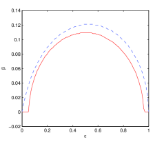
(a) “Three-dimensional” parameter regime.

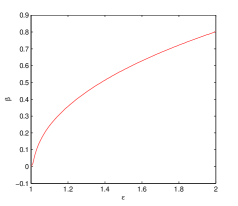
(b) “Two-dimensional” parameter regime.

Figure 1. The biffurcation diagram $\beta$ vs. $\epsilon$. The dashed line indicates the appearance of one real negative eigenvalue of the matrix $J_{N}$, which happens only in the regime $0<\epsilon<1$ (a). The solid line shows the point at which the real part of two conjugate complex eigenvalues of $J_{N}$ become negative. This bifurcation disappears in the “three-dimensional” parameter regime (a) at $0\leq\epsilon\leq 0.05$ and $0.97\leq\epsilon\leq 1$. Observe that for positive viscosity $\nu$ the solution ${\textbf{u}}^{N}$ is linearly stable for every $N$ at $\epsilon=1$, which can be shown rigorously.

For other values of the parameters, we substitute $\lambda=2$, and write the characteristic polynomial of the matrix $J_{N}$

$$x^{4}-\frac{325}{16}\beta x^{3} +\Big{(}4\epsilon^{2}-\frac{19}{4}\epsilon+1+\frac{4497}{64}\beta^{2}\Big{)}x^{2}-$$

$$-\Big{(}\frac{325}{16}\beta^{2}+\frac{5}{4}\epsilon^{2}+\frac{257}{16}-\frac{197}{16}\epsilon\Big{)}\beta x+$$

$$+(\epsilon^{3}-\epsilon^{2})+\Big{(}1+\frac{239}{16}\epsilon+\frac{1}{16}\epsilon^{2}+\beta^{2}\Big{)}\beta^{2}=0.$$ (30)

Next, by fixing an $\epsilon$, we find the largest $\beta$ when the real part of the roots of the polynomial (30) changes its sign. The result of this calculation is shown at Figure $1$.

For every $\epsilon$ in the “three-dimensional” subrange of parameters $0.05<\epsilon<0.97$, there are two bifurcation points. First, there exists a value of $\beta$ for which one of the real eigenvalues of $J_{N}$ crosses $0$ and becomes negative. Further decreasing $\beta$ we observe another bifurcation at which real part of a pair of complex conjugate eigenvalues becomes negative. Therefore, for $0<\epsilon<1$ there exists a function $m(\epsilon)$, such that the matrix $J_{N}$ has $3$ negative eigenvalues for

$$0<\beta=\nu k_{N}^{4}\leq m(\epsilon),$$ (31)

or in other words, for $N$ satisfying

$$4N\leq\log_{\lambda}\nu^{-1}+\log_{\lambda}m(\epsilon),$$ (32)

Note, that $m(\epsilon)>0$, at $\epsilon\in(0.05,0.97)$, and $m(\epsilon)=0$ otherwise.

For the range of parameters $0<\epsilon\leq 0.05$ and $0.97\leq\epsilon<1$ we observe only one bifurcation point at which one of the real eigenvalues becomes negative. Therefore, we call this regime – the “non-chaotic” range of parameters and the reason for that will be explained further.

Finally, for the “two-dimensional” range of parameters $1<\epsilon<2$ the scenario is a little different, as we observe only one bifurcation point at which real part of a pair of complex conjugate eigenvalues becomes negative. Namely, for $1<\epsilon<2$ there exists a function $d(\epsilon)$, such that the matrix $J_{N}$ has $2$ negative eigenvalues for

$$0<\beta=\nu k_{N}^{4}\leq d(\epsilon),$$ (33)

or equivalently, for $N$ satisfying

$$4N\leq\log_{\lambda}\nu^{-1}+\log_{\lambda}e(\epsilon).$$ (34)

In this case we also have, $e(\epsilon)>0$ for all $\epsilon\in(1,2]$, and $d(1)=0$.

4.2. Calculating the lower bound of the dimension of the attractor

In the previous section we show that the Sabra shell model has at most three unstable direction for the “single-mode” forcing. Therefore, we need other type of the force to get a large number of unstable direction, and finally, the lower-bound for the dimension of the global attractor, which would be close to the upper-bound calculated in [5]. Let us define the forcing

$${\textbf{g}}=\sum_{j=1}^{\infty}{\textbf{f}}^{5j},\;\;\;\lvert{\textbf{g}}\rvert=\nu\frac{1}{\lambda^{5}\sqrt{1-\lambda^{-10}}},$$ (35)

where ${\textbf{f}}^{5j}$ is defined in (25). Then the stationary solution corresponding to that forcing is

$${\textbf{u}}^{{\textbf{g}}}=\sum_{j=1}^{\infty}{\textbf{u}}^{5j},$$ (36)

where ${\textbf{u}}^{5j}$ is defined in (26). Using the results of the previous section on the stability of the single-mode stationary solution we conclude that for $0<\epsilon<1$, the number of the unstable directions of the solution ${\textbf{u}}^{{\textbf{g}}}$ equals to $3N/5$, where $N$ satisfies the relation (32). On the other hand, the number of the unstable directions of the solution ${\textbf{u}}^{{\textbf{g}}}$ for $1<\epsilon<2$ equals to $2N/5$, where $N$ satisfies relation (34).

Recall the definition of the generalized Grashoff number (4), which in our case satisfies

$$G=\frac{\lvert{\textbf{g}}\rvert}{\nu^{2}\lambda^{3}}=\frac{1}{\nu\lambda^{8}\sqrt{1-\lambda^{-10}}}.$$

Therefore, we can rewrite the bounds (32) and (32) in terms of the generalized Grashoff number to obtain

$$4N=\log_{\lambda}\nu^{-1}+\log_{\lambda}f(\epsilon)\leq\log_{\lambda}G+\log_{\lambda}f(\epsilon),$$ (37)

where $f(\epsilon)$ denotes $m(\epsilon)$ or $d(\epsilon)$. Therefore, we proved the following statement.

Theorem 2.

The Hausdorff and fractal dimensions of the global attractor $\mathcal{A}$ of the Sabra shell model of turbulence with $\nu>0$ and the forcing defined in (35) satisfies

$$\dim_{F}(\mathcal{A})\geq\dim_{H}(\mathcal{A})\geq K\log_{\lambda}G+\log_{\lambda}f(\epsilon),$$ (38)

for the positive constant $K$ depending on $\epsilon$ satisfying

$$K(\epsilon)=\left\{\begin{array}[]{ll}\frac{3}{20},&\text{for }\;\;0.05<\epsilon<0.97,\\ \frac{1}{10},&\text{for }\;\;1<\epsilon\leq 2,\\ \frac{1}{20},&\text{for }\;\;0<\epsilon\leq 0.05,\;\;\;\text{and}\;\;0.97\leq\epsilon<1,\\ \end{array}\right.$$ (39)

and some positive real function $f(\epsilon)$, which is $0$ only for $\epsilon=1$.

The lower bounds for the global attractor, given by the last Theorem do not match exactly the upper bounds which were obtained previously in [5], namely

$$\dim_{H}(\mathcal{A})\leq\dim_{F}(\mathcal{A})\leq\frac{1}{2}\log_{\lambda}G-C(\epsilon),$$ (40)

where the function $C(\epsilon)$ stays positive and bounded for every $\epsilon\in(0,2)$. Moreover, the constant $K$ in front of the $\log_{\lambda}G$ term, although can be slightly improved, cannot be brought much closer to $\frac{1}{2}$ to match the upper bound of (40).

5. Existence of a trivial global attractor for any value of $\nu$

It is well known that the attractor for the $2$-dimensional space-periodic Navier-Stokes equation with a particular form of the forcing can consists of only one function. This well-known example is due to Yudovich [22] and independently by Marchioro [15] (for the proof see also [7]). The same is true for the Sabra shell model for $1<\epsilon<2$, therefore, we need to stress that the bounds that we obtained for the dimension of the global attractor are valid only for the particular type of forcing that we used in our calculations.

We mentioned in the introduction that for the $2$-dimensional parameters regime the inviscid Sabra shell model without forcing conserves the following quantity

$$\lvert A^{\gamma}u\rvert^{2}=\sum_{n=1}^{\infty}k_{n}^{4\gamma}\lvert u_{n}\rvert^{2},$$

for $4\gamma=-\log_{\lambda}(\epsilon-1)$. For $m>0$ we denote by ${\textbf{P}}_{m}$ – the projection onto the first $m$ coordinates of the sequence u, and ${\textbf{Q}}_{m}={\textbf{I}}-{\textbf{P}}_{m}$.

Theorem 3.

Suppose that the forcing f acts only on the $N$-th shell for some $N\geq 1$. Let ${\textbf{u}}(t)$ be the solution of the the equation (6) in the “two-dimensional” regime of parameters $1<\epsilon<2$, such that for $\gamma=-\frac{1}{4}\log_{\lambda}(\epsilon-1)$ we have

$$Re({\textbf{B}}({\textbf{u}},{\textbf{u}}),{\textbf{A}}^{2\gamma}{\textbf{u}})=0.$$

Then

$$\limsup_{t\to\infty}\lvert{\textbf{Q}}_{m}{\textbf{u}}(t)\rvert^{2}\leq C\frac{1}{k_{m+1}^{4\gamma}}\liminf_{t\to\infty}\lvert{\textbf{P}}_{m}{\textbf{u}}(t)\rvert^{2},$$ (41)

for $C=\frac{k_{N}^{4\gamma}-k_{1}^{4\gamma}}{1-\lambda^{-4\gamma}}$ and $m\geq N$.

Proof.

Taking the scalar product of the equation (6) with u and with ${\textbf{A}}^{2\gamma}{\textbf{u}}$ we get two equations

$$\frac{1}{2}\frac{d}{dt}\lvert{\textbf{u}}\rvert^{2}+\nu({\textbf{A}}{\textbf{u}},{\textbf{u}})=Re(f_{N}u_{N}^{*}),$$

and

$$\frac{1}{2}\frac{d}{dt}\lvert{\textbf{A}}^{\gamma}{\textbf{u}}\rvert^{2}+\nu({\textbf{A}}{\textbf{u}},{\textbf{A}}^{2\gamma}{\textbf{u}})=Re(k_{N}^{4\gamma}f_{N}u_{N}^{*}).$$

Multiplying the energy equation by $k_{N}^{4\gamma}$ and subtracting it from the last equation we get

$$\frac{1}{2}\frac{d}{dt}(\lvert{\textbf{A}}^{\gamma}{\textbf{u}}\rvert^{2}-k_{N}^{4\gamma}\lvert{\textbf{u}}\rvert^{2})+\nu(\lvert{\textbf{A}}^{\gamma+1/2}{\textbf{u}}\rvert^{2}-k_{N}^{4\gamma}\lVert{\textbf{u}}\rVert^{\vphantom{1}}{}^{2})=0.$$ (42)

On the other hand,

$$\lvert{\textbf{A}}^{\gamma+1/2}{\textbf{u}}\rvert^{2}-k_{N}^{4\gamma}\lVert{\textbf{u}}\rVert^{\vphantom{1}}{}^{2} =\sum_{n=1}^{\infty}k_{n}^{2}(k_{n}^{4\gamma}-k_{N}^{4\gamma})\lvert u_{n}\rvert^{2}\geq$$

$$\geq k_{N}^{2}\sum_{n=1}^{\infty}(k_{n}^{4\gamma}-k_{N}^{4\gamma})\lvert u_{n}\rvert^{2}=k_{N}^{2}(\lvert{\textbf{A}}^{\gamma}{\textbf{u}}\rvert^{2}-k_{N}^{4\gamma}\lvert{\textbf{u}}\rvert^{2}).$$

Plugging the last expression into (42) yields

$$\frac{d}{dt}(\lvert{\textbf{A}}^{\gamma}{\textbf{u}}\rvert^{2}-k_{N}^{4\gamma}\lvert{\textbf{u}}\rvert^{2})\leq-2\nu k_{N}^{2}(\lvert{\textbf{A}}^{\gamma}{\textbf{u}}\rvert^{2}-k_{N}^{4\gamma}\lvert{\textbf{u}}\rvert^{2}),$$

and therefore,

$$\limsup_{t\to\infty}(\lvert{\textbf{A}}^{\gamma}{\textbf{u}}(t)\rvert^{2}-k_{N}^{4\gamma}\lvert{\textbf{u}}(t)\rvert^{2})=0.$$ (43)

Finally,

$$\lvert{\textbf{Q}}_{m}{\textbf{u}}\rvert^{2} =\sum_{i=m+1}^{\infty}\lvert u_{i}\rvert^{2}=\sum_{i=m+1}^{\infty}\frac{k_{i}^{4\gamma}-k_{N}^{4\gamma}}{k_{i}^{4\gamma}-k_{N}^{4\gamma}}\lvert u_{i}\rvert^{2}\leq$$

$$\leq\frac{1}{k_{m+1}^{4\gamma}-k_{N}^{4\gamma}}(\lvert{\textbf{Q}}_{m}{\textbf{A}}^{\gamma}{\textbf{u}}\rvert^{2}-k_{N}^{4\gamma}\lvert{\textbf{Q}}_{m}{\textbf{u}}\rvert^{2})=$$

$$=\frac{1}{k_{m+1}^{4\gamma}-k_{N}^{4\gamma}}\bigg{(}(\lvert{\textbf{A}}^{\gamma}{\textbf{u}}\rvert^{2}-k_{N}^{4\gamma}\lvert{\textbf{u}}\rvert^{2})-(\lvert{\textbf{P}}_{m}{\textbf{A}}^{\gamma}{\textbf{u}}\rvert^{2}-k_{N}^{4\gamma}\lvert{\textbf{P}}_{m}{\textbf{u}}\rvert^{2})\bigg{)}\leq$$

$$\leq\frac{1}{k_{m+1}^{4\gamma}-k_{N}^{4\gamma}}\bigg{(}(\lvert{\textbf{A}}^{\gamma}{\textbf{u}}\rvert^{2}-k_{N}^{4\gamma}\lvert{\textbf{u}}\rvert^{2})+(k_{N}^{4\gamma}-k_{1}^{4\gamma})\lvert{\textbf{P}}_{m}{\textbf{u}}\rvert^{2}\bigg{)},$$

and the result follows from (43).

∎

Corollary 1.

The global attractor of the Sabra shell model of turbulence in the “two-dimensional” regime of parameters $1<\epsilon<2$ with the force applied only to the first shell

$${\textbf{f}}^{1}=(f,0,0,\dots),$$ (44)

is reduced to a single stationary solution

$${\textbf{u}}^{1}=(\frac{f}{\nu k_{1}^{2}},0,0,\dots).$$

Proof.

Let ${\textbf{u}}=(u_{1},u_{2},\dots)$ be a solution of the Sabra shell model with the forcing f defined by (44). Then it immediately follows from Theorem 3 that

$$\limsup_{t\to\infty}\lvert{\textbf{Q}}_{1}{\textbf{u}}\rvert^{2}=0,$$

which means that $\limsup_{t\to\infty}\lvert u_{n}\rvert=0$, for every $n\geq 2$.

Define ${\textbf{v}}=(v_{1},v_{2},\dots)$ as ${\textbf{v}}={\textbf{u}}-{\textbf{u}}^{1}$, which satisfies the equation

$$\frac{d{\textbf{v}}}{dt}+\nu{\textbf{A}}{\textbf{v}}+{\textbf{B}}({\textbf{u}},{\textbf{u}})=0,$$

where we used the fact that ${\textbf{B}}({\textbf{u}}^{1},{\textbf{u}}^{1})=0$. Taking the inner product of the equation with the vector ${\textbf{P}}_{1}{\textbf{v}}=(v_{1},0,0,\dots)$ we get that $\lvert v_{1}(t)\rvert^{2}$ satisfies

$$\frac{1}{2}\frac{d}{dt}\lvert v_{1}(t)\rvert^{2}+\nu k_{1}^{2}\lvert v_{1}(t)\rvert^{2}+v_{1}(t)u_{2}(t)u_{3}(t)=0.$$

Using the fact that $u_{2}(t),u_{3}(t)$ tend to $0$ as $t\to\infty$ we conclude that $\lvert v_{1}(t)\rvert^{2}\to 0$ as $t\to\infty$. Therefore,

$$\limsup_{t\to\infty}\lvert{\textbf{v}}\rvert^{2}=\limsup_{t\to\infty}\lvert{\textbf{u}}-{\textbf{u}}^{1}\rvert^{2}=0.$$

finishing the proof. ∎

6. Conclusion

In this work we obtained lower bounds for the dimension of the global attractor of the Sabra shell model of turbulence for specific choices of the forcing term. Our main result states that for these specific choices of the forcing term the Sabra shell model has a large attractor for all values of the governing parameter $\epsilon\in(0,2)\setminus\{1\}$. We also showed the scenario of the transition to chaos in the model, which is slightly different for the two- and three-dimensional parameters regime. In addition, in the three-dimensional parameters regime, $\epsilon\in(0,1)$, we found that when the parameter $\epsilon$ becomes sufficiently close to $0$ or to $1$ where the chaotic behavior in the vicinity of the stationary solution changes dramatically.

Finally, we show that in the “two-dimensional” parameters regime the Sabra shell model has a trivial attractor reduced to a single equilibrium solution for any value of viscosity $\nu$, when the forcing is applied only to the first shell. This result is true also for the two-dimensional NSE due to Yudovich [22] and independently by Marchioro [15] (see also [7]).

References

- [1] A. V. Babin, M. I. Vishik, Attractors of partial differential equations and estimates of their dimension, Uspekhi Mat. Nauk, 38 (1983), 133-187 (in Russian); Russian Math. Surveys, 38, 151-213 (in English).
- [2] L. Biferale, Shell models of energy cascade in turbulence, Annual Rev. Fluid Mech., 35 (2003), 441-468.
- [3] L. Biferale, A. Lambert, R. Lima, G. Paladin, Transition to chaos in a shell model of turbulence, Physica D, 80 (1995), 105–119.
- [4] T. Bohr, M. H. Jensen, G. Paladin, A. Vulpiani, Dynamical Systems Approach to Turbulence, Cambridge University press, 1998.
- [5] P. Constantin, B. Levant, E. S. Titi, Analytic study of the shell model of turbulence, Physica D, 219 (2006), 120-141.
- [6] P. Constantin, B. Levant, E. S. Titi, A note on the regularity of inviscid shell models of turbulence, submitted.
- [7] C. Foias, O. Manley, R. Rosa, R. Temam, Navier-Stokes Equations and Turbulence, Cambridge University press, 2001.
- [8] U. Frisch, Turbulence: The Legacy of A. N. Kolmogorov, Cambridge University press, 1995.
- [9] E. B. Gledzer, System of hydrodynamic type admitting two quadratic integrals of motion, Sov. Phys. Dokl., 18 (1973), 216-217.
- [10] L. Kadanoff, D. Lohse, N. Schröghofer, Scaling and linear response in the GOY turbulence model, Physica D, 100 (1997), 165–186.
- [11] J. Kockelkoren, F. Okkels, M. H. Jensen, Chaotic behavior in shell models and shell maps, J. Stat. Phys., 93, (1998), 833.
- [12] L. D. Landau, E. M. Lifschitz, Fluid Mechanics, Pergamon, Oxford 1977.
- [13] V. X. Liu, A sharp lower bound for the Hausdorff dimension of the global attractors of the 2D Navier-Stokes equations, Commun. Math. Phys., 158, (1993), 327-339.
- [14] V. S. L’vov, E. Podivilov, A. Pomyalov, I. Procaccia, D. Vandembroucq, Improved shell model of turbulence, Physical Review E., 58 (2) (1998), 1811-1822.
- [15] C. Marchioro, An example of absence of turbulence for any Reynolds number, Comm. Math. Phys., 105 (1986), 99-106.
- [16] L. D. Meshalkin and Y. G. Sinai, Investigation of the stability of a stationary solution of a system of equations for the plane movement of an incompressible viscous liquid, J. Appl. Math. Mech., 25 (1961), 1700–1705.
- [17] K. Okhitani, M. Yamada, Temporal intermittency in the energy cascade process and local Lyapunov analysis in fully developed model of turbulence, Prog. Theor. Phys., 89 (1989), 329-341.
- [18] R. Temam, Infinite-Dimensional Dynamical Systems in Mechanics and Physics, Springer-Verlag, New-York, 1988.
- [19] M. Yamada, K. Okhitani, Lyapunov spectrum of a chaotic model of three-dimensional turbulence, J. Phys. Soc. Jpn., 56 (1987), 4210–4213.
- [20] M. Yamada, K. Okhitani, Lyapunov spectrum of a model of two-dimensional turbulence, Phys. Rev. Let., 60 (11) (1988), 983–986.
- [21] M. Yamada, K. Okhitani, Asymptotic formulas for the Lyapunov spectrum of fully developed shell model turbulence, Phys. Rev. E, 57 (6) (1998), 57–60.
- [22] V. I. Yudovich, Example of the generation of a secondary stationary or periodic flow when there is loss of stability of the laminar flow of a viscous incompressible fluid, J. Appl. Math. Mech., 29 (1965), 527 -544.