Exploring an opinion network for taste prediction: an empirical study

Abstract

We develop a simple statistical method to find affinity relations in a large opinion network which is represented by a very sparse matrix. These relations allow us to predict missing matrix elements. We test our method on the Eachmovie data of thousands of movies and viewers. We found that significant prediction precision can be achieved and it is rather stable. There is an intrinsic limit to further improve the prediction precision by collecting more data, implying perfect prediction can never obtain via statistical means.

1 Introduction

With the advent of the World Wide Web (WWW) we witness the onset of what is often called ’Information Revolution’. With so many sources and users linked together instantly we face both challenges and opportunities, specially for scientists. The most prominent challenge is information overload: no one can possibly check out all the information potentially relevant for him. The most promising opportunity is that the WWW offers possibility to infer or deduce other users experience to indirectly boost a single user’s information capability. Both computer scientists and internet entrepreneurs extensively use various collaborative-filtering tools to tap into this opportunity.

The so-called web2.0 represents a new wave in web applications: many newer web sites allow users’ feedback, enable their clustering and communication. Much of users’ feedback can be interpreted as votes or evaluation on the information sources. Such voting is much more widespread: our choice of movies, books, consumer products and services could be considered as our votes representing our tastes. With a view to develop a prediction-model suitable for web application, we need to first test a model is a limited setting. For a more concrete example consider opinions of movie-viewers on movies they have seen. We use in this work the EachMovie dataset, generously provided by the Compaq company. The Eachmovie dataset comprises ratings on $1628$ movies by $72916$ users. The dataset has a density of approximately $3\%$, meaning that $97\%$ of possible ratings are absent. This dataset can represented by an information matrix: each user has only seen a tiny fraction of all the movies; each movie has been seen by a large number of users but they are only a tiny fraction of all users. This (sparse) information matrix has $97\%$ elements missing; our task is to find whether we can predict them leveraging affinity relations hidden in the dataset.

2 Prediction Algorithm and Results

There is a particular way how such information on movies could be used to recommend other users movies they have not yet seen but which would likely suit their tastes. Such recommendations can be made by a centralized agent (matchmaker) who collects a large number of votes. The idea behind such services (called “recommender system” or “collaborative filtering” by computer scientists [1][2][3][4] ) is that users’ votes are first used to measure the affinity of users’ tastes. Then opinions of users with tastes sufficiently similar to the user in question are summed up to predict the opinion on movies she/he has not seen yet. The data of the “matchmaker” are stored in the voting matrix $V$ with entries $v_{i\alpha}$, this is the vote of user $i$ to movie $\alpha$. For simplicity we only take into account from the original data users who have seen at least $200$ movies. As a further approximation we shall compress the original votes $(1to5)$ to $v_{i\alpha}\in\{-1,1\}$, i.e, $1$ and $2$ are converted to $-1$ (dislike), $4$ and $5$ to $1$ (like), $3$ is interpreted as 0, as if the user has not seen the movie. Elsewhere we show that such simplifying approximations do not induce statistically significant reduction in prediction power. The dimension of the rectangular matrix $V$ is $(1223\times 1648)$, i.e. there are $N=1223$ users and $M=1648$ movies. In this matrix there are $\sum_{i,\alpha}|v_{i\alpha}|\sim 2\cdot 10^{5}$ non-zero elements (votes).

Duality picture. The voting matrix $V$ can be viewed in two ways. In user-centric view we measure the pairwise affinity of users. The affinity distribution indicates how much information redundancy is buried in the data to predict users’ opinion about a movie. This is similar to Newman’s ’Ego-centered networks’ [5]. In the movie-centric view we look at the distribution of movie affinity. This shows how controversial movies were voted by the population. This “duality picture” is not symmetric Fig.(1).

Let us start with the user-centric view. We define the overlap between users $i$ and $j$ as

$$\Omega_{ij}=\frac{\sum_{\alpha=1}^{M}v_{i\alpha}v_{j\alpha}}{\sum_{\alpha=1}^{M}|v_{i\alpha}||v_{j\alpha}|},\quad\Omega_{ij}\in(-1,1).$$ (1)

This measures the affinity between users $i$ and $j$. $\Omega_{ij}$ close to $1$ means similar tastes, whereas $\Omega_{ij}$ close to $-1$ means opposite tastes. $\sum_{\alpha=1}^{M}|v_{i\alpha}||v_{j\alpha}|$ gives the number of commonly seen movies by both users $i$ and $j$. $|\cdot|$ denotes the absolute.

In the movie-centric view the affinity between two movies is defined in an analogous way as follows:

$$\Omega_{\alpha\beta}=\frac{\sum_{i=1}^{N}v_{i\alpha}v_{i\beta}}{\sum_{i=1}^{N}|v_{i\alpha}||v_{i\beta}|},\quad\Omega_{\alpha\beta}\in(-1,1).$$ (2)

$\Omega_{\alpha\beta}$ close to $1$ means that movie $\alpha$ and movie $\beta$ are judged as similar by each user, whereas $\Omega_{\alpha\beta}$ close to $-1$ indicates that the two movies are judged to be opposite. $\sum_{i=1}^{N}|v_{i\alpha}||v_{i\beta}|$ gives the number of people who have seen both movies $\alpha$ and $\beta$.

Figure 1: Distribution $P_{u}(d)=\sum_{i}\sum_{j\neq i}\delta(d_{ij},d)/N(N-1)$ of distance between users and the distribution $P_{m}(d)=\sum_{\alpha}\sum_{\beta\neq\alpha}\delta(d_{\alpha\beta},d)/M(M-1)$ of distance between movies. $\delta(d_{x},d)$ is the Kronecker symbol, $N$ is the total number of people in the population and $M$ is the total number of movies.

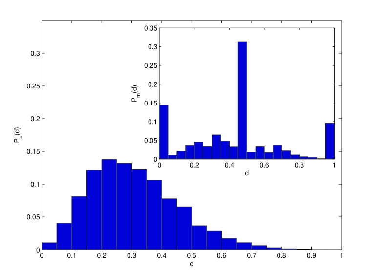
A more intuitive concept is given by the distance $d_{ij}=(1-\Omega_{ij})/2$ for users and $d_{\alpha\beta}=(1-\Omega_{\alpha\beta})/2$ for movies respectively. $d_{ij}\sim 0$ represents similar tastes for user $i$ and user $j$ whereas $d_{ij}\sim 1$ opposite opinions. Likewise interpretations for the movie-centric view.

$P_{u}(d)$ in Fig.(1)indicates a rather homogenous distribution of tastes among users. Furthermore the peak around $d\sim 0.2$ implies a rich information source which allows taste prediction. If users would vote in a random manner the peak would be around $0.5$. On the other hand in the movie-centric view the distribution $P_{m}(d)$ in Fig.(1) appears more polarized. One explanation for this is the following: the overlaps of the users are typically averaged over a lot of bits (from every user there are at least 200 opinions known), while many movies are only few times voted. Hence it is much easier to get a “perfect” $+1$ or $-1$ overlap. Apart from this we observed two effects which also give hints about the asymmetry between the two views. One example: for a Star wars movie the set of ’antipodes’- movie with $d\sim 1$ includes A) some movies oriented for the audience of young women (e.g. Mr. Wrong); B) Less successful sequels of the Star Wars trilogy hated by some of their fans. It is not surprising that for movies of type B there exists a considerable number of people who saw both of them. What is more surprising is that for some of the movies of type $A$ the number of users liking Star Wars could also be quite large. We tentatively attribute it to the ‘girl-friend effect’ in which Star Wars fans were dragged by their girlfriends to see a movie like Mr. Wrong. Most of them disliked it (hence the distance between these movies is close to $1$ in spite of a relatively large common audience).

One can use the information of distances between movies to make a proposition to users: if user $i$ likes movie $\alpha$ ($v_{i\alpha}=1$) and this movie is within a distance $d\sim 0$ with movie $\beta$ it is very likely that user $i$ also will like movie $\beta$.

However to predict a vote $v_{i\alpha}$ we will use the information of affinity between users. Here, user $i$ is the ’center’ of the universe and all others have certain distances to him. Users close to him are more trustful because they share similar tastes. Hence they should have more weight in the prediction. Furthermore we have to penalize users who have not seen that much movies in common. In this way we take care of the statistical significance.

We introduce our method to predict votes: the dataset of votes (matrix $V$) is divided into a ’training’ set $V_{train}$ and a ’test’ set $V_{test}$. The votes of the two sets are generated randomly out of the voting matrix $V$. The votes in $V_{train}$ are treated as observed whereas the votes in $V_{test}$ are hidden for the algorithm. That is we use votes in $V_{train}$ to predict votes in $V_{test}$.

For prediction we use the following form

$$v^{\prime}_{i\alpha}=\frac{\sum_{j\neq i}\Omega_{ij}\sqrt{\omega_{ij}}}{\sum_{j\neq i}|\Omega_{ij}|\sqrt{\omega_{ij}}}\cdot\frac{v_{j_{\alpha}}}{|v_{j\alpha}|}.$$ (3)

Where $v^{\prime}_{i\alpha}$ is the predicted vote which has to be compared to $v_{i\alpha}\in V_{test}$. $v_{j\alpha}\in V_{train}$ are the votes which are supposed as known . Statistical significance is taken into account by $\omega_{ij}=\sum_{\alpha}|v_{i\alpha}||v_{j\alpha}|$, which is the number of shared movies between user $i$ and user $j$. Our measure of accuracy is given by

$$s_{i\alpha}=\left\{\begin{array}[]{ll}1&\textrm{ if $sign(v^{\prime}_{i\alpha})=v_{i\alpha}$}\\ 0&\textrm{ otherwise}\end{array}\right.,\Pi=\frac{\left(\sum_{i}\sum_{\alpha}s_{i\alpha}\right)}{|V_{test}|}$$ (4)

Where $\Pi\in(0.5,1.0)$, $|V_{test}|$ is the number of votes we want to predict and $v_{i\alpha}\in V_{test}$.

$\Pi\sim 0.5$ means no predictive power. In this case prediction is random whereas $\Pi=1$ gives an accuracy of $100\%$ (every vote was predicted correctly).

It is a common belief that prediction accuracy in ’recommender systems’ is an increasing function of the available amount of data. The more votes the better. However, our result shows a saturation of the prediction power after a critical mass of data Fig.(2).

Figure 2: The prediction power $\Pi(\rho)$ as a function of $\rho$. $\rho$ is the fraction of present votes in $V_{train}$ to the total number of votes in the voting matrix $V$.

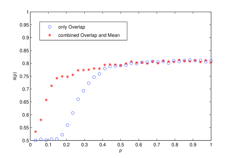
We can clearly distinguish two phases. In the region $\rho\leq 0.2$ no reasonable prediction can be done, because there are not enough overlaps present. In this region the prediction is by chance. By increasing the number of votes in $V_{train}$ - the prediction accuracy increases too. However, after a critical value of $\rho\sim 0.6$ the predictability saturates, without any further improvement with additional data input. When we use somewhat different method with the mean tendance as an aide, that is

$$v^{\prime}_{i\alpha}=\bar{v_{\alpha}}+\frac{\sum_{j\neq i}\Omega_{ij}\sqrt{\omega_{ij}}}{\sum_{j\neq i}|\Omega_{ij}|\sqrt{\omega_{ij}}}\cdot\frac{v_{j_{\alpha}}}{|v_{j\alpha}|}.$$ (5)

the onset of the plateau is much earlier, in a sense this represents a big improvement. $\bar{v_{\alpha}}=\sum_{i}v_{i\alpha}/N_{\alpha}$ denotes the average vote of a movie $\alpha$ and $N_{\alpha}$ is the number of people who voted for movie $\alpha$. However the plateau value remains the same. This hints some fundamental limit at work, for this we need examine the origins of noise intrinsically buried in the data. First of all, the massive collection of thousands web surfers is far from being a precise process, an average user often votes carelessly, and with biases and whim, typical of any human experiment. However if a rater sometimes votes random, and random data won’t show any meaningful correlation, as pointed out by [6], on the aggregate one must expect that there is some coherence left in the data, its less-than-perfect collection quality finally shows up in our calculation. It is remarkable that this degree of imperfection can be calculated at all. Though we should never expect perfection in human endeavors, but significant room left for improvement. Prediction quality can never attain $1$, no matter how good is the method and data [7].

We investigate in more detail what are crucial parameters for prediction accuracy. Fig.(3) shows a non cumulative and a cumulative plot of the prediction power. In the non cumulative case we only take into account users within a certain range of distance. Predicting $v_{i\alpha}$ (the vote from user $i$ to movie $\alpha$) we build a subset of users $A^{(i)}_{d_{l}}=\{j\neq i|d_{l}\leq d_{ij}\leq d_{l}+0.1\}$ and use only members of this set to predict votes in question. $d_{l}\in\{0.0,0.1\cdots,0.9\}$ is the lower distance threshold. The upper distance threshold is given by $d_{l}+0.1$. Prediction power is given again by Eq.(4). For the cumulative case $d_{l}$ remains always $0$ and we vary only the upper distance threshold. We build a subset of users $B^{(i)}_{d_{u}}=\{j\neq i|0.0\leq d_{ij}\leq d_{u}\}$ to predict vote $v_{i\alpha}$. $d_{u}\in\{0.1,0.2,\cdots,1.0\}$ denotes the upper distance threshold.

Figure 3: The prediction power $\Pi(d_{l})$ as a function of the lower distance threshold for the non cumulative case and $\Pi(d_{u})$ as a function of the upper threshold (small box) for the cumulative case. Note that the calculated accuracy for the non cumulative case is plotted always between the lower and the upper distance threshold.

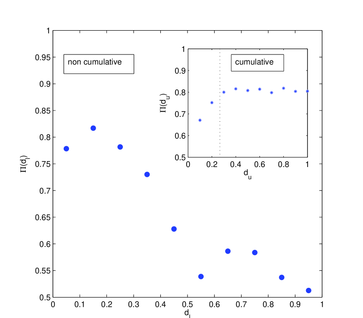
We observe in the non cumulative case that my ‘antipodes’ Fig.(3) still could be used for prediction (albeit poorly). However users who are very similar to ’me’ are best in predicting my tastes. The number of users within a small distance $d$ to a given user is low but their predictions are good, while the number of users at intermediate distances $d\sim 0.3$ is large but their predictive power is poor. One needs to strike a balance. As one can see in the cumulative case Fig.(3) prediction power saturates around $d=0.2$ (indicated by the dotted line). So there is no harm in including the votes from all users (provided that we weight them as we do).

Next we investigate what determines the mean predictability of a user or a movie Fig.(4). People who have a small average distance $\bar{d_{i}}=\sum_{j\neq i}d_{ij}/(N-1)$ to the rest of the population are better predictable then people who have somewhat special tastes. If somebody follows the mainstream he or she will have more users with similar tastes which are best for predictions. Note that the predictability seems to extrapolate to $1$ for small $d$.

Figure 4: The prediction power $\Pi(d)$ as a function of the mean distance $d$ and the predictability $\Pi(N)$ for movies as a function of the number of votes $N$ it has (small box). The two plots are non cumulative. An example: $\Pi(0.2)$ gives the average predictability of users who have an average distance $\bar{d_{i}}=\sum_{j\neq i}d_{ij}/(N-1)\leq d=0.2$ to the rest of the population, $\Pi(0.3)$ gives the average predictability of users who have an average distance $d=0.2\leq\bar{d_{i}}=\sum_{j\neq i}d_{ij}/(N-1)\leq d=0.3$ and so on. The plot for the movie predictability (small box) is also non cumulative and indicates an increasing prediction accuracy for an increasing number of votes.

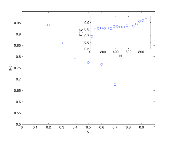
The major determinant of predictability of a movie is how many votes it has. This is quantified in Fig.(4). It could be interpreted like this: the prediction of an opinion of a given user on a popular movie could be based on large ensemble of other users who also saw this movie. Chances are that this ensemble would contain decent number of users with tastes similar to the user we are currently trying to predict. Thus the prediction would turn out to be more precise.

3 Conclusion

To conclude we note that our relatively straightforward method can yield significant prediction precision. However there seems to have an intrinsic limit in the precision that should be attributed to the original noisy source. Our results reveal that people’s tastes tend to be homogenous whereas movies are polarized. The implications of our study go much beyond merely predicting user’s tastes. One can image that consumers’ relation with myriad of products and services as a much larger information matrix. It would have significant impact on the economy if a consumer’s potential tastes to the vast majority of products and services that she has not yet tested can, to a reasonable precision, be predicted. With the rapid evolution of the Information Technology, where the feedbacks from consumers can be effectively tracked and analyzed, it is not to far-fetched to see our economy completed transformed by a new paradigm.

References

- [1] P. Resnick, N. Iacovou, M. Suchak, P. Bergstrom, J. Riedl, Grouplens: an open architecture for collaborative filtering of netnews, in: Proceedings of the 1994 ACM conference on Computer supported cooperative work, 1994.
- [2] J. Breese, D. Heckerman, C. Cadie, Empirical analysis of predictive algorithms for collaborative filtering, in: Proceedings of the 14th Annual Conference on Uncertainty in Artificial Intelligence (UAI-98), 1998.
- [3] D. Billsus, M. Pazzani, Learning collaborativ information filters, in: Proceedings of the 14 Conference on Uncertainty in Reasoning, 1998, pp. 43–52.
- [4] B. Sarwar, G. Karypis, J. Konstan, J. Reidl, Item-based collaborative filtering recommendation algorithms, in: WWW ’01: Proceedings of the tenth international conference on World Wide Web, 2001.
- [5] M. Newman, Ego-centered networks and the ripple effect, Social Networks 25 (2001) 83–95.
- [6] S. Maslov, Y.-C. Zhang, Extracting hidden information from knowledge networks, Phys. Rev. 87 (2001) 248701.
- [7] W. Hill, L. Stead, M. Rosenstein, G. Furnas, Recommending and evaluating choices in a virtual community of use, in: Proceedings of the SIGCHI conference on Human factors in computing systems, 1995.