High-order harmonic generation with a strong laser field and an attosecond-pulse train: the Dirac Delta comb and monochromatic limits

Abstract

In recent publications, it has been shown that high-order harmonic generation can be manipulated by employing a time-delayed attosecond pulse train superposed to a strong, near-infrared laser field. It is an open question, however, which is the most adequate way to approximate the attosecond pulse train in a semi-analytic framework. Employing the Strong-Field Approximation and saddle-point methods, we make a detailed assessment of the spectra obtained by modeling the attosecond pulse train by either a monochromatic wave or a Dirac-Delta comb. These are the two extreme limits of a real train, which is composed by a finite set of harmonics. Specifically, in the monochromatic limit, we find the downhill and uphill sets of orbits reported in the literature, and analyze their influence on the high-harmonic spectra. We show that, in principle, the downhill trajectories lead to stronger harmonics, and pronounced enhancements in the low-plateau region. These features are analyzed in terms of quantum interference effects between pairs of quantum orbits, and compared to those obtained in the Dirac-Delta limit.

I Introduction

One attosecond (10${}^{-18}s$) is roughly the time it takes for light to travel through atomic distances. This fact makes high-frequency pulses of attosecond duration a very powerful tool for resolving or even controlling dynamic processes occurring at the atomic scale AdiM2004 . Indeed, in the past few years, such pulses have caused a breakthrough in metrology, with applications as diverse as resolving the motion of bound electrons atto1 , exciting inner-shell electrons atto2 , inducing vibrational wavepackets in molecules atto3 , or controlling electron emission atto4 .

Attosecond pulses have been predicted theoretically in the mid-1990s saclay96 and have become experimentally feasible a few years later attoexptrain ; attoexp ; mairesse . They are a direct consequence of the fact that high-order harmonics, generated by the interaction of a strong laser field (intensities of the order of $10^{14}\mathrm{W/cm}^{2}$) with a gaseous sample, are almost phase locked saclay96 . Hence, by superposing sets of high harmonics, it is possible to produce attosecond pulses. Specifically, there exist two main scenarios: either one obtains an attosecond-pulse train, by employing long input pulses attoexptrain ; mairesse , or isolated attosecond pulses, from few-cycle driving fields attoexp ; fewcyclerev ; atto1 . Both situations have been widely exploited in the literature, and sometimes the attosecond pulses appear in combination with additional driving fields.

For instance, recently, an attosecond-pulse train superposed to a strong, infrared, linearly polarized field has been employed to control high-harmonic generation (HHG) atthhg2004 ; dpg and above-threshold ionization (ATI) attati2005 . Such a train exhibited a time-delay $t_{d}$ with respect to the infra-red field. By varying this delay, one could influence several features, such as the intensities, resolutions, and maximal energies in the high-harmonic or photoelectron spectra. This scheme has been proposed theoretically atthhg2004 ; attati2005 and realized experimentally attati2005 ; dpg , and the key idea behind it is to provide an additional pathway, which can be controlled, for an electronic wave packet to be released in the continuum.

This can be understood in view of the physical mechanisms behind both phenomena. At a time $t^{\prime},$ an electron is freed by tunneling or multiphoton ionization. Subsequently, it propagates in the continuum, gaining energy from the field, and it is driven back towards its parent ion, to which it returns at a time $t$. If the electron recombines or rescatters, there is either emission of high-frequency radiation (i.e., HHG), or of high-energy photoelectrons (i.e., high-order ATI) tstep . For low-order ATI peaks, the electron reaches the detector without rescattering. An attosecond pulse train allows the electron to reach the continuum by absorbing high-energy photons and being able to overcome the ionization potential. Additionally, since they are of very short duration, the attosecond pulses provide a tool to control the instant at which the electron is being ejected. This has direct consequences in the momentum it acquires from the field when it is released attati2005 , and also a strong influence on the kinetic energy the electron has upon return atthhg2004 ; dpg . Therefore, it also affects the spectra.

The results in atthhg2004 ; dpg and attati2005 have been obtained from the numerical solution of the time-dependent Schrödinger equation, and the attosecond-pulse train has been modeled by the superposition of five harmonics ($\Omega_{11}=11\omega$ to $\Omega_{19}=19\omega$). These are realistic assumptions, and well within the available experimental data. However, in order to interpret the results obtained, the attosecond-pulse train has been approximated by a monochromatic wave of frequency $\Omega_{15}=15\omega,$ which is the central frequency of the group of harmonics in question, and a classical model for an electron ejected by such a wave and propagating in a strong, low-frequency field was constructed. These simplifications have enormously facilitated the understanding of the ionization mechanisms, and, specifically, have shown how to manipulate ionization by varying the time delay $t_{d}.$

In a previous publication, we have also investigated the ATI and HHG spectra from an atom irradiated by a time-delayed attosecond-pulse train superposed to a near-infrared laser field FSVL2006 . Specifically, we have considered the transition amplitudes for both phenomena within the Strong-Field Approximation, and took the attosecond pulse train to be a sum of Dirac-Delta functions in the time domain. These assumptions have allowed an almost entirely analytical treatment, which has been vital for a clear understanding of the problem. Indeed, we were able to investigate the influence of the attosecond pulses on the spectra in far more detail than in atthhg2004 ; dpg ; attati2005 , and to interpret the results obtained in terms of quantum interference effects.

To a very large extent, our results, as well as their physical interpretation, agree with those in atthhg2004 ; dpg ; attati2005 . In fact, we have obtained, for very specific time delays, enhancements of more than one order of magnitude in the harmonic spectra similar to those reported in atthhg2004 . Furthermore, as the time delay increases, the enhancements move gradually from the high-order harmonics towards lower frequencies, until they only affect the low-plateau region. Finally, for ATI, we have observed an identical behavior of the yield with the time delay as in attati2005 , namely that it extends towards higher energies if $\omega t_{d}=n\pi$, and that it decays most quickly, as the frequency increases, for $\omega t_{d}=(2n+1)\pi/2$.

There exist, however, a few discrepancies, especially for HHG, between our results and those in atthhg2004 . First, the above-mentioned features occur for different phases $\phi=\omega t_{d}$. Second, the explanations for such features are slightly different. In FSVL2006 , we related the enhancements in the spectra to a particular pair of orbits, for which the excursion times $\Delta t=t-t^{\prime}$ of the electron in the continuum were very short. Therefore, the spreading of the electronic wave packet in the continuum would be very reduced. Hence, the overlap of this wave packet, upon return, with the bound state it left, would be considerable, leading to very prominent harmonics. We have shown that the maximal kinetic energy the electron may have upon return, for this pair of orbits, was very much dependent on the delay between the infra-red field and attosecond-pulse train, going from $1.8U_{p}$, where $U_{p}$ is the ponderomotive energy, to vanishingly small values. In the former case, this leads to strong harmonics throughout, whereas the latter case causes enhancements only in low-energy regions of the spectra.

In Ref. atthhg2004 , however, the modifications in the spectra have been attributed to the selection of specific electron trajectories, which are present in case it is released by a high-frequency wave, and, subsequently, propagates in a strong infra-red field. In comparison to the case in which the electron is released only by the infrared field, there is a splitting in the electron orbits, into the so-called ”downhill” and ”uphill” trajectories, with respect to the effective potential barrier $V_{\mathrm{eff}}=V(r)-\mathbf{r}.\mathbf{E}(t^{\prime})$ at the electron start time $t^{\prime}$, where $\mathbf{E}(t^{\prime})$ and $V(r)$ denote the electric field and the atomic binding potential, respectively. The former and the latter case relate to the situation for which the electron velocity, at $t^{\prime}$, has the opposite or the same direction of the field, respectively. If the time delays are appropriately chosen, one may enhance ionization, and thus the HHG spectra, for a particular set of orbits, or for none.

Probably, such discrepancies are rooted on the fact that the attosecond pulse train has been modeled in different ways. While in atthhg2004 it has been approximated by a monochromatic wave, in FSVL2006 we considered a Dirac-Delta comb. In this context, one should keep in mind that a realistic attosecond-pulse train possesses a broad frequency range. Therefore, a monochromatic wave is as much as an approximation as a Dirac-Delta comb. The main difference lies in the number of harmonics composing the train: the former should work better if this number is small (such as in atthhg2004 ), and the latter if it is large.

In this proceeding, we present a detailed discussion of the two limits which one may adopt, when modeling the attosecond pulse train. We put a particular emphasis on the consequences of taking the attosecond pulse train to be a monochromatic wave, within the Strong-Field Approximation, for high-order harmonic generation. In order to make an assessment of the similarities and differences from the Dirac Delta comb employed in our previous work FSVL2006 , we will also briefly recall such results.

This manuscript is organized as follows: In Sec. II, we present the explicit expressions for the transition amplitudes, if the attosecond pulse train is taken to be a monochromatic wave (Sec. II.1) or a Dirac Delta comb (Sec. II.2). In particular, we discuss how the saddle-point equations are modified for each case, and relate their solutions to the classical orbits of an electron in a field. Subsequently, in Sec. III, we compute such orbits explicitly, and employ them to calculate high-harmonic spectra. Finally, in Sec. IV we conclude the paper, relating both limits to the results in atthhg2004 .

II Transition amplitudes

The general expression for the HHG transition amplitude, in the strong-field approximation footnsfa , is given by

$$M_{\Omega} = i\int_{-\infty}^{\infty}dt\int_{-\infty}^{t}~{}dt^{\prime}\int d^{3}kd_{z}^{\ast}(\mathbf{k}+\mathbf{A}(t))d_{z}(\mathbf{k}+\mathbf{A}(t^{\prime}))$$ (1)

$$E(t^{\prime})\exp[iS(t,t^{\prime},\Omega,\mathbf{k})],$$

with the action

$$S(t,t^{\prime},\Omega,\mathbf{k})=-\frac{1}{2}\int_{t^{\prime}}^{t}[\mathbf{k}+\mathbf{A}(\tau)]^{2}d\tau-I_{p}(t-t^{\prime})+\Omega t,$$ (2)

where $\mathbf{A}(t),$ $\Omega,\mathbf{k}$ and $I_{p}$ denote the vector potential, the harmonic frequency, the intermediate momentum of the freed electron and the atomic ionization potential, respectively hhgsfa . Eq. (1) describes a physical process in which an electron is freed at a time $t^{\prime}$, propagates in the continuum with momentum $\mathbf{k}$ from $t^{\prime}$ to $t$, and, at this time, recombines with its parent ion, generating a harmonic of frequency $\Omega$. The prefactors

$$d(\mathbf{k}+\mathbf{A}(t))=\left\langle\psi_{0}\right|\mathbf{r}.\mathbf{\epsilon}_{x}\left|\mathbf{k}+\mathbf{A}(t)\right\rangle$$ (3)

and

$$d^{\ast}(\mathbf{k}+\mathbf{A}(t^{\prime}))=\left\langle\mathbf{k}+\mathbf{A}(t^{\prime})\right|\mathbf{r}.\mathbf{\epsilon}_{x}\left|\psi_{0}\right\rangle,$$ (4)

where $\left|\psi_{0}\right\rangle$ and $E(t^{\prime})=-dA(t^{\prime})/dt^{\prime}$ denote the electronic bound state and the electric field at the time the electron is released, respectively, contain all the influence of the atomic binding potential, which is implicit in the bound-state wave functions. In general, the vector potential is given by $\mathbf{A}(t)=\mathbf{A}_{l}(t)+\mathbf{A}_{h}(t),$ and the total electric field by $\mathbf{E}(t)=\mathbf{E}_{l}(t)+\mathbf{E}_{h}(t)$, where the indices $l$ and $h$ refer to the laser field and the attosecond pulses, respectively. In this paper, we work within the so-called “broad gaussian limit”, which implies that the electron is bound, and returns to, a bound state localized at the origin of the coordinate system hhgsfa . This yields constant prefactors (3) and (4).

For low enough frequencies and high enough laser intensities, Eq. (1) can be solved to a good approximation by the steepest descent method. Thus, we must determine $\mathbf{k}$, $t^{\prime}$ and $t$ so that $S(t,t^{\prime},\Omega,\mathbf{k})$ is stationary, i.e., so that its partial derivatives with respect to these parameters vanish. Apart from considerably simplifying the computations involved, this approximation has the advantage of providing a clear space-time picture for the physical process in question, and allowing a detailed assessment of quantum-interference effects. Furthermore, as it will be shown below, the saddle-point equations can be related to those describing the classical orbits of an electron orbitshhg .

If the attosecond pulses are absent, the saddle-point equations read

$$\left[\mathbf{k}+\mathbf{A}_{l}(t^{\prime})\right]^{2}=-2I_{p}$$ (5)

$$2(\Omega-I_{p})=\left[\mathbf{k}+\mathbf{A}_{l}(t)\right]^{2},$$ (6)

and

$$\int_{t^{\prime}}^{t}d\tau\left[\mathbf{k}+\mathbf{A}_{l}(\tau)\right]=0.$$ (7)

Eq. (5) and (6) give the energy conservation at the start and recombination times, respectively, while Eq. (7) yields the intermediate electron momentum fulfilling the condition for the electron to return. The first equation expresses tunneling ionization at $t^{\prime},$ and has no real solution. Physically, this means that tunneling has no classical counterpart. In the limit of $I_{p}\rightarrow 0,$ this equation describes a classical electron being released with vanishing drift velocity. Eq. (6) illustrates a process in which the kinetic energy of the electron upon return is converted into a photon of frequency $\Omega$. Near the cutoff, whose energy position corresponds to the maximal value this quantity may take, such a process has no classical counterpart, and the transition probability is expected to decay exponentially.

We will now include the attosecond-pulse train. The strong, low-frequency field will be approximated by a linearly polarized monochromatic wave of amplitude $E_{0}$, i.e.,

$$\mathbf{E}_{\mathrm{l}}(t)=E_{0}\sin\left(\omega t\right)\mathbf{\epsilon}_{x},$$ (8)

while the attosecond-pulse train will be taken as

$$\mathbf{E}_{\mathrm{h}}(t)=\frac{E_{\mathrm{h}}}{{\sigma(t)}}\sum_{q=2k_{0}+1}^{2k_{1}+1}\sin\left[q\omega(t-t_{d})\right]\mathbf{\epsilon}_{x},$$ (9)

of amplitude $E_{\mathrm{h}}$. Eq. (9) is a sum over several odd high-order harmonics, which are phase-locked and exhibit a time delay $t_{d}$ with respect to the background field. The indices $2k_{0}+1$ and $2k_{1}+1$ yield the minimal and the maximal harmonic order, respectively. The function $\sigma(t)$ denotes the train temporal envelope, which will be taken as $\sigma=const.$ Physically, this corresponds to an infinitely long attosecond-pulse train.

In our model, we assume that the attosecond pulses will mainly influence the electron ejection in the continuum but not its subsequent propagation. This latter step will be governed by the low-frequency field. For this reason, unless stated otherwise, we will use the approximation $E(t^{\prime})\simeq E_{\mathrm{h}}(t^{\prime})$ in the prefactor of Eq. (1), but not in the action. This implies that the vector potential is approximated by $\mathbf{A}(t)\simeq\mathbf{A}_{l}(t).$

II.1 The monochromatic limit

For a finite number of harmonics, this yields highly oscillating prefactors, which are no longer slowly varying. Hence, they must be incorporated in the action. The HHG transition amplitude then reads

$$M_{\mathrm{h}}=-\frac{E_{\mathrm{h}}}{2i\sigma}\sum_{q=2k_{0}+1}^{2k_{1}+1}M_{\mathrm{h}}^{(q)},$$ (10)

with

$$M_{\mathrm{h}}^{(q)} = \int_{-\infty}^{\infty}dt\int_{-\infty}^{t}dt^{\prime}\int d^{3}kd^{\ast}(\mathbf{k}+\mathbf{A}_{l}(t))d(\mathbf{k}+\mathbf{A}_{l}(t^{\prime}))$$ (11)

$$(e^{iq\omega(t^{\prime}-t_{d})}-e^{-iq\omega(t^{\prime}-t_{d})})\exp[iS(t,t^{\prime},\Omega,\mathbf{k})].$$

In Eq. (10), we will define a modified action,

$$\tilde{S}=S\pm q\omega(t^{\prime}-t_{d}).$$ (12)

This leads to changes in the saddle-point equation (5), which now reads

$$\left[\mathbf{k}+\mathbf{A}_{l}(t^{\prime})\right]^{2}=2(\mp q\omega-I_{p}).$$ (13)

Thereby, the solution in $-q\omega$ does not make physically sense, and thus will not be taken into account, whereas that in $+q\omega$ describes an ionization process in which an electron is ejected by the absorption of a high-frequency photon. Hence, the attosecond-pulse train, in which a superposition of such processes occurs, provides an alternative pathway for the electron to reach the continuum. This is in agreement with the discussions in atthhg2004 . We will consider here the limit for which the attosecond pulse train is described by a monochromatic wave, so that the sum in (10) is dropped.

If Eq. (13) is combined with (6) and (7), one obtains the expressions

$$\omega t^{\prime}=\epsilon_{1}\arccos\alpha$$ (14)

and

$$\epsilon_{2}\sqrt{1-\alpha^{2}}-\sin\omega t =$$

$$= \omega(\epsilon_{1}\arccos\alpha-t)(\cos\omega t-\gamma_{2}),$$

with $\alpha=\cos\omega t+\gamma_{1}-\gamma_{2},$ and $\epsilon_{i}=\pm 1$ $(i=1,2),$ for the electron ionization and return  times, respectively. Hence, the problem of finding the pairs of times $(t,t^{\prime})$ has been reduced to solving the transcendental equation (II.1). In the above-stated equations, one may identify the parameters

$$\text{ }\gamma_{1}=\pm\sqrt{\frac{\Omega-I_{p}}{2U_{p}}}\text{ and }\gamma_{2}=\pm\sqrt{\frac{q\omega-I_{p}}{2U_{p}}}.$$ (16)

In particular $\gamma_{2}$ is very important for determining the initial conditions for the electron when it is being ejected in the continuum.

One should note that there exist sign ambiguities in the above-stated equations. Furthermore, additional complications may be caused by the fact that $\arccos\alpha=$ $\arccos(2n\pi-\alpha).$ We will discuss such problems explicitly in Sec. III.1, in which they are overcome by means of physical arguments.

II.2 The Dirac-Delta limit

In the limit $k_{1}-k_{0}\longrightarrow\infty$, which is the main assumption in our former work FSVL2006 , Eq. (9) reads

$$\mathbf{E}_{\mathrm{h}}(t)=\frac{E_{h}\pi}{\sigma}\sum_{n=0}^{\infty}(-1)^{n}\delta(\omega(t-t_{d})-n\pi)\mathbf{\epsilon}_{x}.$$ (17)

This yields the transition amplitude

$$M_{\mathrm{h}}^{(D)} = \frac{i\pi E_{\mathrm{h}}}{\sigma}\sum_{n=0}^{\infty}(-1)^{n}\int_{-\infty}^{+\infty}dt\int d^{3}k\exp\left[iS(t,t_{n}^{\prime},\Omega,\mathbf{k})\right]$$ (18)

$$d_{z}^{\ast}(\mathbf{k}+\mathbf{A}_{l}(t))d_{z}(\mathbf{k}+\mathbf{A}_{l}(t_{n}^{\prime})).$$

In this case, the ionization time is being fixed at $t_{n}^{\prime}=t_{d}+n\pi/\omega$. The above-stated equation means, physically, that the electron is no longer reaching the continuum through tunneling ionization, but is being released by the attosecond pulses. However, in contrast to the approximation in the previous section, all information about the velocity with which the electron is leaving is lost. Indeed, the electron is reaching the continuum with any of the energies $N\omega-I_{p}$, since all harmonics composing the train are equivalent.

Under these assumptions, the transition amplitude is further simplified so that only the integrals in the intermediate electron momentum $\mathbf{k}$ and the return time $t$ must be solved. In this case, the saddle-point equations (6) and (7) can be combined in order to obtain the transcendental equation

$$\sin\omega t-(-1)^{n}\sin\omega t_{d}$$ (19)

$$= \left[\omega(t-t_{d})-n\pi\right]\left(\cos\omega t-\gamma_{1}\right),$$

where $\gamma_{1}$ is defined in (16). Similarly to the monochromatic-limit case, one may identify ambiguities in Eq. (19). It turned out, however, that they are fewer and far easier to overcome in the limit discussed in this Section.

III Results

III.1 Start and return times

We will now assess the influence of the additional attosecond-pulse train on the electron orbits. As a starting point, we will approximate it by a high-frequency monochromatic wave. In general, we will refer to a pair of orbits employing the indices $(i,j)$, which increase with the electron excursion times $\Delta t=t-t^{\prime}$ in the continuum.

We will initially concentrate on the shortest pair of orbits, i.e., $(1,2)$, which provide the most prominent contributions to the high-harmonic spectra. In Fig. 1, we display the real parts of the ionization and return times for such orbits, obtained from the saddle point equations (13), (6) and (7), as compared to the situation for which the attosecond pulses are absent (i.e., for $q=0$ in (13)). In all cases, start and return times occur in pairs, which coalesce at well-defined energies. Such energies correspond to the maximal kinetic energy with which a classical electron may return to its parent ion. For higher energies, the transition amplitudes are exponentially decaying. Hence, potentially, such energies lead to cutoffs in the spectra. For a monochromatic field in the absence of the attosecond-pulse train, the cutoff occurs at $3.17U_{p}+I_{p}.$

In the figure, we can identify two main distinct regimes. If the frequency $\Omega_{q}=q\omega$ is lower than the ionization potential $I_{p}$, qualitatively, there is the same behavior for the start times $t^{\prime}$ or return times $t.$ Indeed, the only difference is the cutoff energy, which is slightly lower. An inspection of Eqs. (14)  and (II.1) supports this interpretation: if $q\omega-I_{p}<0$, the parameter $\gamma_{2}$ is purely imaginary, so that the solutions of (II.1) occur in conjugate pairs. The element of such a pair which leads to $\mathrm{Im}[t^{\prime}]<0$ is discarded as unphysical, whereas the other element is directly associated with the tunneling process. In this context, the quantity $\mathrm{Im}[t^{\prime}]$ provides information about how probable the tunneling process is, as it will be discussed below.

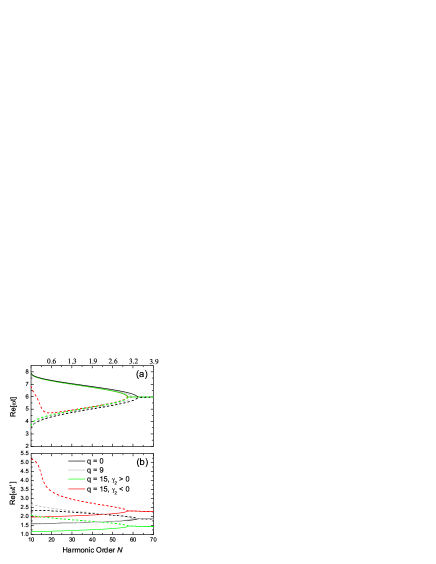
Figure 1: (Color Online) Real parts of return and start times (panel (a) and (b), respectively), as functions of the high-harmonic order, for the two shortest orbits of an electron subject to a monochromatic field of intensity $I=4\times 10^{14}\mathrm{W/cm^{2}}$, and frequency $\omega=0.057$ a.u., superposed to a high-frequency, monochromatic wave of $I_{h}=I/10$, approximated by a monochromatic wave of frequency $\Omega_{q}=q\omega$. For comparison, we also provide such times for the case in which the attosecond train is absent ($q=0$ in Eq.(13)). The atomic system is taken to be argon ($I_{p}=0.58$ a.u.) and we only show the harmonic orders for which $\Omega>I_{p}$. The dashed and the solid lines in the figure refer to the orbit $1$ and $2$, respectively. The numbers on the upper edge of the figure denote the kinetic energy of the electron upon return, in units of the ponderomotive energy $U_{p}$.

If on the other hand, $q\omega-I_{p}>0$ (for instance, for $q=15)$, the attosecond pulses have given enough energy for the electron to overcome the potential barrier. In this case, it is reaching the continuum with velocity $v=\pm\sqrt{2(q\omega-I_{p})}.$ In comparison to a situation for which the electron is being released with vanishing velocity, which is the classical limit of Eq. (5), there is a splitting in the ionization times $t^{\prime}$ for each set of orbits. This is precisely the effect reported in Ref. atthhg2004 , and can be readily understood from Eq. (II.1), in which now the parameter $\gamma_{2}$ is real. Hence, there exist now two solutions of (II.1) which make physically sense. The solution with $\gamma_{2}<0$ yields the downhill trajectories in atthhg2004 , whereas that with $\gamma_{2}>0$ corresponds to the uphill trajectories.

Interestingly, however, for both types of trajectories, the electron returns almost at the same time $t$. In fact, there are only noticeable differences near the ionization threshold $\Omega=10\omega$, which, at most, will influence the low-plateau region. Hence, the electron excursion times in the continuum are considerably shorter for $\gamma_{2}<0$. Obviously, the larger the frequency $\Omega_{q}=q\omega,$ the more pronounced the splitting is. In comparison with atthhg2004 , however, there is a much larger overlap of the start times for both types of trajectories near the ionization threshold.

From a more technical viewpoint, it is worth mentioning that, in the computation of the orbits $(1,2)$, we have taken $\epsilon_{1}=\epsilon_{2}=+1$ and $\gamma_{1}<0$ in general. As an exception, for $q=15$, $\gamma_{2}<0$, and $i=1$, for harmonic frequencies $\Omega/\omega\leq 24.4$ one must employ an analytical continuation in Eq. (II.1), with $\epsilon_{2}=-1,$ $\epsilon_{1}=+1$ and $2\pi-\arccos\alpha$ instead of $\arccos\alpha,$ in order to guarantee continuous solutions.

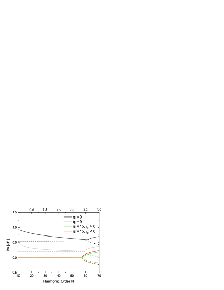
Figure 2: (Color online) Imaginary parts of electron start times for the two shortest orbits of an electron subject to the same field and atomic parameters as in the previous figure. In the figure, we only show the harmonic orders for which $\Omega>I_{p}$. The dashed and the solid lines in the figure refer to the orbit $1$ and $2$, respectively. The numbers on the upper edge of the figure denote the kinetic energy of the electron upon return, in units of the ponderomotive energy $U_{p}$.

The above-stated physical interpretation is confirmed by Fig. 2, in which the imaginary parts of the start times are depicted. Such imaginary parts are in a sense a measurement of a quantum-mechanical process having a classical counterpart. Indeed, the smaller $|\mathrm{Im}[t^{\prime}]|$ is, the larger the probability that the process in question takes place will be. In the figure, we observe that, for the monochromatic and $q=9$ cases, $|\mathrm{Im}[t^{\prime}]|\neq 0.$ This is expected, since tunneling ionization has no classical counterpart. Furthermore, $|\mathrm{Im}[t^{\prime}]|$ decreases if the attosecond pulses are present, due to an effectively narrower barrier. In case the electron is able to overcome the atomic binding potential (e.g., for $q=15$), for energies lower than the cutoff, $|\mathrm{Im}[t^{\prime}]|$ is vanishingly small, since now a classical counterpart does exist. Clearly, beyond the cutoff energy, the imaginary parts of such times increase.

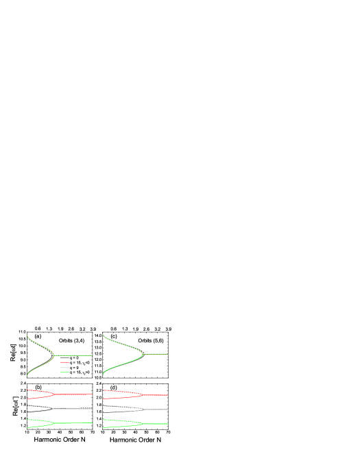
Figure 3: (Color online) Real parts of start and return times for the pairs of orbits $(3,4)$ [panels (a) and (b)], and $(5,6)$ [panels (c) and (d)], as functions of the high-harmonic order, for the same atomic and field parameters as in the previous figures. The orbits $(3,4)$ have been obtained by taking $\epsilon_{1}=\epsilon_{2}=+1$ and $\gamma_{1}>0$ in Eq. (II.1), while $(5,6)$ have been found employing $\epsilon_{1}=\epsilon_{2}=+1$ and $\gamma_{1}<0$. The numbers on the upper edge of the figure denote the kinetic energy of the electron upon return, in units of the ponderomotive energy $U_{p}$.

The splitting in the electron start times is not exclusive of $(1,2)$, but, in fact, occurs for all pairs of orbits. As concrete examples, in Fig. 3 we illustrate the real parts of the start and return times for the orbits $(3,4)$ and $(5,6).$ Such orbits correspond to electron excursion times $\Delta t\sim 1.5T$ and $\Delta t\sim 2T,$ respectively, where $T=2\pi/\omega$ denotes a cycle of the driving field. Clearly, the start times $t^{\prime}$ split for $q\omega-I_{p}>0,$ due to the electron non-vanishing velocity upon ejection. Once more, each pair of start times leads to a shorter and a longer set of orbits, which correspond to $\gamma_{2}<0$ or $\gamma_{2}>0$, respectively. The corresponding electron start times do not overlap in any energy region. This is due to the fact that they are much more localized than for the orbits $(1,2).$

For comparison, in Fig. 3, we present the solutions of Eq. (19), obtained when the attosecond-pulses are approximated by a sum of Dirac-Delta functions, for several time delays. The start and return times, as well as the cutoff energies, are different from those in the previous figures. Indeed, we no longer observe a splitting in the sets of ionization and recombination times, as compared to the situation for which the attosecond pulses are absent. This is in perfect agreement with the fact that now there is no longer a well-defined velocity with which the electron is being ejected. In contrast, however, there is now a single ionization time per half cycle, determined by Eq. (17). The return times, however, still occur in pairs that coalesce at the cutoffs. For each pair of orbits, the cutoff energies, as well as the excursion times, considerably changes with the time delay $t_{d}$.

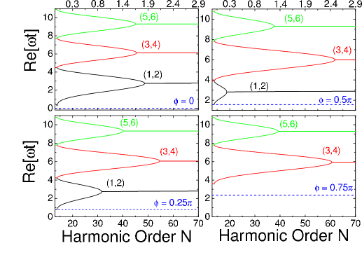
Figure 4: (Color online) Real part of the recombination times as a function of the high-harmonic order, for neon ($I_{p}=0.79$ a.u.) interacting with a monochromatic field of intensity $I=5\times 10^{14}\mathrm{W/cm^{2}}$, and frequency $\omega=0.057$ a.u. and an attosecond-pulse train of intensity $I_{\mathrm{h}}=10^{13}\mathrm{W/cm^{2}}$, composed of an infinite number of harmonics (Eq. (17)). Parts (a), (b), (c) and (d) correspond to delays $\phi=0$, $\phi=0.25\pi$, $\phi=0.5\pi$ and $\phi=0.75\pi$ between the attosecond-pulse train and the low-frequency driving wave, respectively. In the figure, we only show the harmonic orders for which $\Omega>I_{p}$, and the pairs of orbits are indicated by the natural numbers $(i,j)$, which increase according to the electron excursion time in the continuum. The ionization times are indicated by the blue dashed lines, and the numbers on the upper edge of the figure give the approximate kinetic energy of the electron upon return, in units of the ponderomotive energy $U_{p}$.

III.2 Harmonic spectra

We will now analyze the spectra computed under the assumptions in Sec. II.1, i.e., that the attosecond-pulse train can be approximated by a high-frequency, monochromatic wave. For comparison, we will also present spectra computed considering that the APT is a sequence of Dirac-Delta functions. In this latter case, however, we will keep the discussion as brief as possible, as a detailed analysis is already presented in FSVL2006 . In both cases, we have employed a uniform saddle-point approximation in order to compute the transition amplitudes. This approximation is discussed in detail in atiuni .

If one concentrates on the physical picture of downhill and uphill trajectories, a very important question is the influence of each type of orbit in the high-harmonic spectra, and how such trajectories can be selected. In atthhg2004 , such a selection has been performed by employing an appropriate time-delay $t_{d}$ between the strong, infra-red field and the attosecond-pulse train. In our framework, however, since we are approximating the train by a monochromatic wave, all information about this parameter is lost. However, we can mimic the effect achieved in atthhg2004 by leaving out, or including, the corresponding orbits in our computations.

In Fig. 5.(a), we present the spectra computed for a train with the frequency $\Omega_{15}=15\omega$ employing all orbits up to $(5,6)$. In this case, $q\omega-I_{p}>0$, so that the electron is being ejected with non-vanishing drift velocity and the spectra contains contributions from both the uphill and the downhill trajectories. We have restricted the electron start times to the first half cycle of the laser field, so that there are no sharp harmonics in the figure. One is able to view, however, the structures caused by the interference between the different pairs of trajectories very clearly. Prominent features are also a cutoff near harmonic order $N=57$. This is in agreement with Fig. 1, which shows that the pairs of orbits (1,2) coalesce around this energy, and also with Fig. 2, for which there is a sharp increase in $|\mathrm{Im}[t^{\prime}]|$ at this harmonic order. Furthermore, there is a very pronounced hump in the low-plateau region.

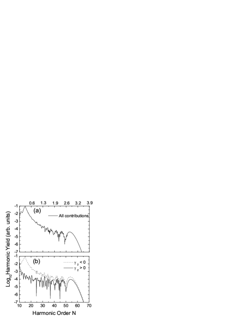
Figure 5: Harmonic spectra computed with the orbits $(1,2)$, $(3,4)$ and $(5,6)$, for an attosecond-pulse train of frequency $\Omega_{15}=15\omega$ superposed to a strong, near-infrared field of frequency $\omega=0.057$ a.u. The field and atomic parameters are the same as in Fig. 1. Panel (a) exhibits the contributions from all sets of orbits, while panel (b) displays the individual contributions from the orbits with $\gamma_{2}>0$ or $\gamma_{2}<0$ in Eq. (II.1). The numbers on the upper edge of the figure give the kinetic energy of the electron upon return, in units of the ponderomotive energy $U_{p}$.

More detail is provided in Fig. 5.(b), in which the individual contributions from the downhill ($\gamma_{2}<0$) and the uphill ($\gamma_{2}>0$) trajectories are displayed. In general, the former contributions are at least half an order of magnitude larger than the latter. This is expected, since, for $\gamma_{2}<0,$ the electron excursion times in the continuum are shorter for all sets of orbits. This means that there is less spreading for the electronic wave packet, and consequently a larger overlap, upon return, between such a wave packet and the atomic bound state with which it recombines. Obviously, this leads to a larger harmonic yield. Furthermore, in both cases there is no difference in the cutoff energy. This is due to the fact that all trajectories split symmetrically, with respect to the purely monochromatic case.

The above-stated features can be understood in detail analyzing the contributions from each pair of orbits. Such contributions are displayed in Fig. 6. For both cases, the main features in the spectra, such as their overall intensities, the plateau shapes and cutoff energies, are determined by the orbits $(1,2)$. In fact, the contributions from such orbits are at least one order of magnitude larger than those from $(3,4)$ or $(5,6)$. This is in particular true for the case $\gamma_{2}<0$, due to the shorter excursion times. Apart from that, they coalesce at a much larger energy than the other sets. This means that, classically, the maximal energy for which the electron returns to its parent ion along $(1,2)$, and consequently the cutoff, is larger than for the longer orbits. In the figure, we also notice that the hump in the low-plateau region, for $\gamma_{2}<0,$ can be traced back to the fact that the electron excursion time in the continuum, for the set $(1,2)$ is extremely short in this case (see, e.g., Fig. 1). The other pairs of orbits mainly contribute to the substructure in the spectra. Another noteworthy feature is that, regardless of the sign of $\gamma_{2}$, the cutoff energies are the same for all sets of orbits, in agreement with the previous discussion.

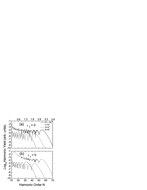
Figure 6: Individual contributions from the shortest three pairs of orbits to the high-harmonic spectra, for the same field and atomic parameters as in the previous figure. Panel (a)  and (b) depicts the contributions from $\gamma_{2}>0$ or $\gamma_{2}<0$ in Eq. (II.1), respectively. For comparison the overall contributions are displayed as the solid black lines in the figure. The numbers on the upper edge of the figure give the kinetic energy of the electron upon return, in units of the ponderomotive energy $U_{p}$.

Another scenario, presented in Fig. 7 for comparison, is observed if the attosecond-pulse train is taken to be a Dirac-Delta comb. In this case, the dominant set of orbits, and, consequently, the shape of the spectra, are highly dependent on the time delay $t_{d}$. For instance, if the time delay is vanishing [Fig. 7.(a)], the spectrum is dominated by the orbits $(1,2)$. This is due to the fact that they coalesce at the energy $I_{p}+1.8U_{p}$, which is at a relatively high harmonic order. Furthermore, since the electron excursion times are very short, the harmonics are quite prominent. For $\phi=\omega t_{d}=0.25\pi$ [Fig. 7.(b)], there is now a double plateau, with two consecutive intensity drops at $I_{p}+0.93U_{p}$ and $I_{p}+2.11U_{p}$. These are the energies for which the orbits $(1,2)$ and $(3,4)$ coalesce, respectively. Specifically in the upper half of the plateau, there was a drop in one order of magnitude, as compared to Fig. 7.(a). This is due to the larger excursion times, and, consequently, wave-packet spreading, for $(3,4)$. If the delay increases further [Fig. 7.(c)], the contributions from $(1,2)$ only cause a shoulder in the spectrum, due to the fact that they now coalesce at $I_{p}+0.26U_{p}$, and the plateau, extending until $I_{p}+2.5U_{p}$, is determined by the orbits $(3,4)$. The latter orbits dominate the spectra even more for $\phi=\omega t_{d}=0.75\pi$ [Fig. 7.(d)], since the cutoff energy for $(1,2)$ is now vanishingly small. This effect is very similar to that observed in atthhg2004 , even though it occurs for completely different delays.

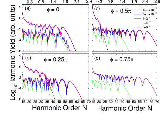
Figure 7: (Color online) Contributions of isolated pairs of orbits to the high-harmonic spectra for the same atomic and external-field parameters in Fig. 4, and delays $\phi=0$, $\phi=0.25\pi$, $\phi=0.5\pi$ and $\phi=0.75\pi$ between the attosecond-pulse train and the low-frequency driving wave (Figs. 7(a), 7.(b), 7.(c) and 7.(d), respectively). In the figure, we only show the harmonic orders for which $\Omega>I_{p}$. The contributions from specific pairs of orbits are depicted in the same colors as those employed in Fig. 4, for depicting each corresponding pair. For comparison, the spectra computed with the ten shortest orbits and with orbit 3 to 10 are given as the thick lines in the figure. The numbers on the upper edges of the figure give the approximate kinetic energy of the electron upon return, in units of the ponderomotive energy $U_{p}$.

IV Conclusions

The outcome of this work supports the results in atthhg2004 in several ways. In general, it also shows that, by changing the initial conditions with which an electron is ejected in the continuum, one may manipulate several features in the spectra, such as the high-harmonic intensities, or cutoff. Furthermore, by considering the electron to be released in the continuum by a monochromatic wave, we have obtained a splitting of the electron start times very similar to that reported in atthhg2004 , within the context of the Strong-Field Approximation, in the so-called uphill and downhill trajectories.

We have also observed enhancements in the low-plateau region, and higher overall intensities for the contributions from the downhill trajectories. This indicates a good perspective for harmonic control, by selecting either the downhill or uphill trajectories with, for instance, an adequate delay between the infrared field and the attosecond-pulse train.

We have also obtained very detailed information about the contributions of specific pairs of orbits to the spectra. In the monochromatic limit, the shortest pair of trajectories, denoted $(1,2)$ is completely dominant, determining the shape of the plateau, the cutoff energy and the overall intensity in the spectra. This is due to the fact that the maximal classical energy for this pair, and thus the cutoff, is always at a higher harmonic order than for the longer pairs of trajectories.

In contrast, in case one considers a sum of Dirac-Delta functions, the dominance of this pair will depend very much on the time delay between the infra-red field and the attosecond pulses. This is due to the fact that the maximal energy an electron returning along these orbits is not always at a higher harmonic frequency than for the longer pairs. For instance, if for $\omega t_{d}=0,$ the orbits (1,2) coalesce at the end of the plateau, and thus overshadow the remaining contributions, for $\omega t_{d}=0.25\pi$ and $\omega t_{d}=0.5\pi,$ this energy lies at the low-energy part of the plateau, or near the ionization potential, respectively. Hence, the orbits (3,4) will also play an important role in the spectra.

A feature in common for both the monochromatic and the Dirac-Delta limits is that the excursion time $\Delta t=t-t^{\prime}$ of the electron in the continuum is a very important parameter, and considerably influences the shape of the plateau and harmonic intensities. This is not surprising, since, now, for all sets of orbits, the electron is reaching the continuum with a roughly equal, and large, probability. Hence, the differences in the yield will be mainly determined by the overlap between the returning electronic wave packet and the bound state with which it recombines. The shorter the orbit along which the electron is returning is, the larger this overlap will be. In contrast, if the electron is released by tunneling ionization, the probability with which it is ejected will depend much more critically on the instantaneous potential barrier, and also influence the yield.

Moreover, it is remarkable that both asymptotic limits exhibit features in common with those obtained in atthhg2004 within a more realistic model for the attosecond pulses. The monochromatic limit, for instance, allows one to identify the downhill and uphill trajectories, and to analyze their consequences in the spectra. Approximating the attosecond pulse train by a sum of Dirac Delta functions, on the other hand, sheds light on several features reported in atthhg2004 , such as a double plateau, or changes of more than one order of magnitude in the harmonic spectra. However, only in Delta-Dirac case there is a decrease in the energy of the enhanced harmonics, with increasing time delays $t_{d}$.

There exist, however, aspects of atthhg2004 that we have not addressed. We have not, for instance, investigated the differences in the high-harmonic resolution, due to a particular trajectory choice. Indeed, in order to do so, it would have been necessary to extend the start times to several cycles of the laser field. Instead, we have restricted them only to the first half cycle, in order to have a closer look at quantum interference effects. Furthermore, the uniform approximation employed in this work requires that we deal with pairs of trajectories (for details see atiuni ), and such effects are expected to be related to single trajectories in a pair saclay96 . These issues were not the main objective of this work, and are open for further studies.

- (1) For a review c.f. P. Agostini and L. DiMauro, Rep. Prog. Phys. 67, 813 (2004).
- (2) M. Hentschel, R. Kienberger, Ch. Spielmann, G.A. Reider, N. Milošević, T. Brabec, P.B. Corkum, U. Heinzmann, M. Drescher and F. Krausz, Nature 414, 509 (2001).
- (3) M. Schnürer, Ch. Streli, P. Wobrauschek, M. Hentschel, R. Kienberger, Ch. Spielmann, and F. Krausz, Phys. Rev. Lett. 85, 3392 (2000); M. Drescher, M. Hentschel, R. Kienberger, M. Uiberacker, V. Yakovlev, A. Scrinzi, T. Westerwahlbesloh, U. Kleineberg, U. Heinzmann, and F. Krausz, Nature 419, 803 (2002).
- (4) H. Niikura, F. Légaré, R. Hasbani, A. D. Bandrauk, M. Yu. Ivanov, D. M. Villeneuve and P. B. Corkum, Nature 417, 917 (2002).
- (5) R. Kienberger, M. Hentschel, M. Uiberacker, Ch. Spielmann, M. Kitzler, A. Scrinzi, M. Wieland, Th. Westerwalbesloh, U. Kleineberg, U. Heinzmann, M. Drescher, F. Krausz, Science 297, 1144 (2002); A. Baltuska, Th. Udem, M. Uiberacker, M. Hentschel, E. Goulielmakis, Ch. Gohle, R. Holzwarth, V. S. Yakovlev, A. Scrinzi, T. W. Hänsch, and F. Krausz, Nature 421, 611 (2003).
- (6) Ph. Antoine, A. L’Huillier and M. Lewenstein, Phys. Rev. Lett. 77, 1234 (1996).
- (7) N. A. Papadogianis, B. Witzel, C. Kalpouzos and D. Charalambidis, Phys. Rev. Lett. 83, 4289 (1999); P. M. Paul, E. S. Toma, P. Breger, G. Mullot, F. Augé, Ph. Balcou, H. G. Muller, and P. Agostini, Science 292, 1689 (2001).
- (8) M. Drescher, M. Hentschel, R. Kienberger, G. Tempea, C. Spielmann, G. A. Reider, P. B. Corkum and F. Krausz, Science 291, 1923 (2001).
- (9) Y. Mairesse, A. de Bohan, L. J. Frasinski, H. Merdji, L. C. Dinu, P. Monchicourt, P. Breger, M. Kovačev, R. Taïeb, B. Carré, H. G. Muller, P. Agostini and P. Salières, Science 302, 1540 (2003).
- (10) For a review c.f. T. Brabec and F. Krausz, Rev. Mod. Phys. 72, 545 (2000).
- (11) K. J. Schafer, M. B. Gaarde, A. Heinrich, J. Biegert, and U. Keller, Phys. Rev. Lett. 92, 023003 (2004); M. B. Gaarde, K. J. Schafer, A. Heinrich, J. Biegert, and U. Keller, Phys. Rev. A 72, 013411 (2005); J. Biegert, A. Heinrich, C. P. Hauri, W. Kornelis, P. Schlup, M. P. Anscombe, M. B. Gaarde, K. J. Schafer and U. Keller, J. Mod. Opt. 53, 87 (2006); J. Biegert, A. Heinrich, C. P. Hauri, W. Kornelis, P. Schlup, M. P. Anscombe, K. J. Schafer, M. B. Gaarde and U. Keller, Laser Physics 15, 899 (2005).
- (12) P. Johnsson, K. Varjú, T. Remetter, E. Gustafsson, J. Mauritsson, R. Lopez-Martens, S. Kazamias, C. Valentin, Ph. Balcou, M. B. Gaarde, K. J. Schafer, and A. L’Huillier, J. Mod. Opt. 53, 233 (2006).
- (13) P. Johnsson, R. López-Martens, S. Kazamias, J. Mauritsson, C. Valentin, T. Remetter, K. Varjú, M. B. Gaarde, Y. Mairesse, H. Wabnitz, P. Salières, Ph. Balcou, K. J. Schafer, and A. L’Huillier, Phys. Rev. Lett. 95, 013001 (2005).
- (14) P. B. Corkum, Phys. Rev. Lett. 71, 1994 (1993); K. C. Kulander, K. J. Schafer, and J. L. Krause in: B. Piraux et al. eds., Proceedings of the SILAP conference, (Plenum, New York, 1993).
- (15) C. Figueira de Morisson Faria, P. Salières, P. Villain and M. Lewenstein, Phys. Rev. A, in press (2006)
- (16) M. Lewenstein, Ph. Balcou, M. Yu. Ivanov, A. L’Huillier and P. B. Corkum, Phys. Rev. A 49, 2117 (1994); W. Becker, S. Long, and J. K. McIver, Phys. Rev. A 41, 4112 (1990); ibid. 50, 1540 (1994); M. Lewenstein, K. C. Kulander, K. J. Schafer and Ph. Bucksbaum, Phys. Rev. A 51, 1495 (1995).
- (17) P. Salières, B. Carré, L. LeDéroff, F. Grasbon, G. G. Paulus, H. Walther, R. Kopold, W. Becker, D.B. Milošević, A. Sanpera and M. Lewenstein, Science 292, 902 (2001).
- (18) The SFA consists in neglecting the atomic potential in the propagation of the electron in the continuum, the laser field when the electron is bound or rescatters, and the excited states of the atom in question.
- (19) C. Figueira de Morisson Faria, H. Schomerus and W. Becker, Phys. Rev. A 66, 043413 (2002).