Localized modes and bistable scattering in nonlinear network junctions

Abstract

We study the properties of junctions created by crossing of $N$ identical branches of linear discrete networks. We reveal that for $N>2$ such a junction creates a topological defect and supports two types of spatially localized modes. We analyze the wave scattering by the junction defect and demonstrate nonzero reflection for any set of parameters. If the junction is nonlinear, it is possible to achieve the maximum transmission for any frequency by tuning the intensity of the scattering wave. In addition, near the maximum transmission the system shows the bistable behaviour.

I Introduction

Recently, a variety of different discrete network systems have been studied in order to find the optimal geometries for enhancing both linear and nonlinear resonant wave transmission chaos ; pre_junction ; prb_molina1 , to reveal the conditions of the prefect reflection and Fano resonances prb_molina2 ; pre_our1 ; pre_our2 , as well as to analyze the soliton propagation in the discrete structures where the role played by the topology of the network becomes important ol_dc ; prl_dc ; phys_d_junction . One of the major issues of those studies is to understand an interplay and competition of topology and nonlinearity in the dynamics and predict new interesting phenomena.

Many of such waveguide structures can be described as discrete linear and nonlinear networks composed of straight, bent, and crossed waveguides in which forward and backward propagating waves become coupled to each other via one or more crossings (or network junctions). The well-known systems for realizing these structures are photonic-crystal circuits prl_fan ; pre_minga , micro-ring resonator structures with more than two coupled channel waveguides josa_sipe , and discrete networks for routing and switching of discrete optical solitons prl_dc . The important question is how the waveguide crossing affects the wave propagation in the network and how we can modify the junction transmission by making it nonlinear.

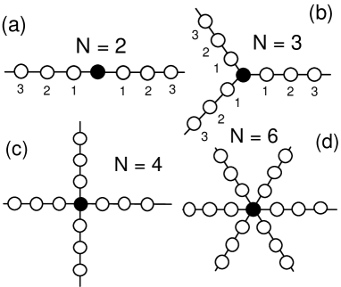
Figure 1: Examples of $N$-branched discrete network junctions.

In this paper, we study the geometry-mediated localized modes and wave scattering in the structures composed of $N$ discrete waveguides (‘branches’) crossing at a common point (‘junction’), as shown schematically in Figs. 1(a-d). This system can have direct applications to the physics of two-dimensional photonic-crystal circuits prl_fan ; pre_minga , and it describes the transmission properties of the $Y$-splitters [see Fig. 1(b)], the waveguide cross-talk effects [see Fig. 1(c)], and other types of photonic-crystal devices. We show that the intersection point of the discrete waveguides acts as a complex $\delta$-like defect even in the absence of any site energy mismatch, i.e. when the crossing point is identical to any of the waveguide points. Therefore, the waveguide junction can be viewed as a topological defect. We show that this new type of defect gives rise to two stable localized modes (or defect modes) at the intersection point, the staggered and unstaggered ones, regardless of the amount of nonlinearity or site energy mismatch at the junction. Next, we study the scattering of plane waves by the crossing point, where the incoming wave propagates along one of the branches, and the waves are scattered to all the branches. In the linear regime, we find that for $N>2$ the reflection coefficient is always nonvanishing. This fundamental limitation prevents us from achieving an ideal $Y$-splitter, unless we optimize and engineer the sites near the junction ol_dc . For a nonlinear junction of the crossed discrete linear waveguides, we reveal the possibility of achieving the maximum transmission for almost any frequency of the incoming plane wave by tuning the input intensity. For some conditions, bistability in the transmission may occur near the transmission maximum. To verify our analytical results obtained for plane waves, we study the propagation of a Gaussian pulse across the junction by direct numerical simulations. The numerical results agree nicely with our analysis.

The paper is organized as follows. In Sec. II we introduce our model. Section III is devoted to the study of the properties of a linear junction, while Sec. IV considers the case of a nonlinear junction and discuss bistability. Our numerical results are summarized in Sec. V, while Sec. VI concludes the paper.

II Model

We consider the system created by $N$ identical discrete linear waveguide (branches) crossed at a common point (junction) which we consider to be linear or nonlinear [see Figs. 1(a-d)]. The corresponding waveguide structure can be described in a general form by the system of coupled discrete nonlinear equations,

$$i\dot{\phi}_{n}^{(k)} = \phi_{n+1}^{(k)}+\phi_{n-1}^{(k)}\;,\;n\geq 1$$

$$\phi_{0}^{(k)} = \phi_{0}\;,$$ (1)

$$i\dot{\phi}_{0} = \sum\limits_{k=1}^{N}\phi_{1}^{(k)}+(\epsilon+\lambda|\phi_{0}|^{2})\phi_{0}\;,$$

where the index $k$ refers to the branch number ($k=1,2,\cdots,N$). In this model, we endow the junction ($n=0$) with a linear impurity $\epsilon_{0}$ and a Kerr nonlinear coefficient $\lambda$. We notice that a similar discrete model can be derived for different types of two-dimensional photonic-crystal devices based on the Green’s function approach pre_minga . In that case, the complex field $\phi_{n}^{(k)}$ corresponds to the amplitude of the electric field.

III Linear junction

First, we consider the linear regime when $\lambda=0$, and all equations (II) are linear. We start our analysis by investigating the possible localized states in the system (II). In order to do that, we look the solutions in the well-known form,

$$\phi_{n}^{(k)} = A\exp\{-\chi|n|-i\Omega\tau\}\;,\;n\geq 0\;,$$ (2)

where $A$ is the mode amplitude, $\tau$ is the corresponding evolution coordinate (time in a general case, or the longitudinal propagation coordinate, for some problems of optics), $\Omega$ is the frequency, and $\chi$ is the spatial (or temporal) decay rate of a localized state. After substituting this solution into Eq. (II), we obtain the relations for the frequency $\Omega$ and the decay rate $\chi$,

$$\Omega = 2\cosh\chi\;,$$

$$e^{\chi} = (N-1)e^{-\chi}+\epsilon_{0}\;.$$ (3)

By denoting $y=e^{-\chi}$, we rewrite the second equation in Eq. (III) as follows

$$(N-1)y^{2}+\epsilon_{0}y-1=0\;,$$ (4)

which, in general, possesses two solutions

$$y^{\pm}={1\over{N-1}}\left(-\frac{\epsilon_{0}}{2}\pm\sqrt{\left(\frac{\epsilon_{0}}{2}\right)^{2}+N-1}\right),$$ (5)

which are of opposite signs $y^{+}>0,y^{-}<0$. As a result, there exist two different solutions of our system

$$\chi^{\pm}=\left\{\begin{array}[]{ll}-\ln y^{+}\\ -\ln|y^{-}|+i\pi,\end{array}\right.$$ (8)

which describe unstaggered or staggered localized states.

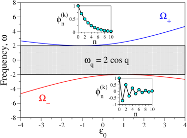
Figure 2: (Color online) Spectrum of linear waves of the system (II) vs. the impurity strength $\epsilon_{0}$ for $N=3$. In addition to the propagating modes $\omega_{q}=2\cos q$, two localized states appear, $\Omega^{\pm}$. At the critical values these localized states touch the band of the propagating modes. Insets show the amplitude profiles of the corresponding staggered and unstaggered modes for $\epsilon_{0}=0$.

In the simplest case of a homogeneous system ($\epsilon_{0}=0$) there exist always two bound states for $N\geq 2$ [see Fig. 2],

$$\chi^{+}=\ln(\sqrt{N-1})\;\;,\;\;\chi^{-}=\ln(\sqrt{N-1})+i\pi\;.$$ (9)

Therefore, the junction itself constitutes an example of a different class of defect: a topological defect. This defect supports two localized states whose decay rates $\chi^{\pm}$ are inversely proportional to the number of branches $N$.

In an inhomogeneous case when $\epsilon_{0}\not=0$, the decay rate of the localized state can change drastically depending on the impurity strength. For example, Eq. (4) supports the solutions $y=1$ (or $\chi=0$), when $\epsilon_{0}=2-N$ and $y=-1$ (or $\chi=i\pi$), when $\epsilon_{0}=N-2$. This means that in these cases one of the localized states can disappear. By looking at the frequency dependence of the localized state $\Omega$ on the impurity strength $\epsilon_{0}$ see Fig. 2], we see that one of the defect modes touches the band of the linear spectrum exactly when the corresponding localized state disappears. This happens precisely at $\epsilon_{0}=\pm(N-2)$.

Now we analyze the transmission properties of this new type of defect. To this end, we consider an incoming plane wave propagating in the branch $k=1$ and calculate the transmitted waves in other branches. We begin by imposing the scattering boundary conditions for Eq. (II),

$$\phi_{n}^{(k)}=e^{-i\omega_{q}\tau}\left\{\begin{array}[]{lc}Ie^{iqn}+re^{-iqn}&n>1,\;k=1\;,\\ te^{iqn}&n>1,\;k>1\;,\end{array}\right.$$ (12)

where $\omega_{q}=2\cos q$ is the the frequency of the incoming plane wave. Continuity condition of the plane wave at the junction implies $I+r=t$. On the other hand, the equation for $\phi_{0}$ can be written in the form,

$$\omega_{q}t=IE^{-iq}+re^{iq}+(N-1)te^{iq}+\epsilon_{0}t\;.$$ (13)

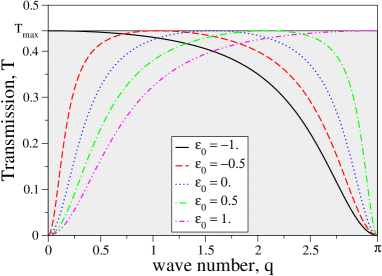
Figure 3: (Color online) Linear transmission coefficient for different values of the impurity strength $\epsilon_{0}$ (and $N=3$). This plot shows that at the critical values $\epsilon_{0}=\pm(2-N)$, the transmission coefficient becomes maximum at the corresponding band edge, $T(0,\pi)=4/N^{2}$, when one of the localized states touches the edge of the linear spectrum [see Fig. 2]. For intermediate values, $2-N<\epsilon_{0}<N-2$, the maximum transmission is inside the propagation band. The shaded area indicates the possible values of the transmission coefficient.

By combining these two conditions, we can obtain the amplitude of the transmitted wave,

$$t=\frac{2i\sin qI}{2i\sin q+\epsilon_{0}+(N-2)e^{iq}}=\frac{2}{N}\frac{I}{1-i\alpha_{q}}\;,$$ (14)

where $\alpha_{q}=(\epsilon_{0}+(N-2)\cos q)/(N\sin q)$. The transmission coefficient for any branch is defined as $T=|t/I|^{2}$. From Eq. (14) we see that even in the homogeneous system ($\epsilon_{0}=0$), the waveguide junction produces an effective geometry-induced complex $\delta$-like scattering potential, $\epsilon_{q}=(N-2)e^{iq}$, which depends on the parameters of the incoming plane wave.

We can write the transmission coefficient in the form

$$T=\frac{4}{N^{2}}\frac{1}{1+\alpha_{q}^{2}}\;,$$ (15)

the reflection coefficient is: $R=1-(N-1)T$. The maximum of the transmission coefficient $T_{\rm max}=4/N^{2}$ can be reached for $\alpha_{q}=0$. We note that $R_{\rm min}=1-4(N-1)/N^{2}>0$ for $N>2$, and it never vanishes. As a result, the $N$-junction system described by the model (II) will always reflect some energy back into the incoming branch. This is a fundamental limitation which does not allow us to build a perfect $Y$-splitter.

At this point, the following natural question arises: What happens in the system at the maximum transmission? First, we notice that this point does not correspond to any resonance. According to the linear scattering theory all (quasi-)bound states of our system can be obtained as poles of the the transmission amplitude (14). The poles can be found in the complex plane from the condition $\alpha_{q}=-i$, by assuming that the wave number $q$ is complex $q=q^{r}+i\chi$. Complex wave numbers correspond to quasi-bound states with the complex frequency $\Omega$, and they can be interpreted as resonances where the real part of the frequency gives the resonance frequency and its imaginary part describes the lifetime (or width) of the resonance. After some algebra, we find that there exist only two solutions for $q^{r}=0,\pi$, and for $\chi$ we have exactly the same solutions as in Eq. (4). This means that our system does not support any quasi-bound states ($0<q^{r}<\pi$), and there exist only two real bound states ($q^{r}=0,\pi$, $\chi\not=0$).

What really happens is quite the opposite. Due to the frequency dependence of the effective scattering potential $\epsilon_{q}$, it simply disappears when the condition $\epsilon_{0}+Re(\epsilon_{q})=0$ (or $\alpha_{q}=0$) is satisfied. And the system becomes almost transparent. The nonzero reflection exists due to the nonzero imaginary part of the effective scattering potential $Im(\epsilon_{q})=(N-2)\sin q$.

Equation for poles of the transmission amplitude $\alpha_{q}=-i$ differs from the equation for the maximum transmission $\alpha_{q}=0$, and there is no relation between them. But, in fact, there exists the condition when these two equations may produce the same results, e.g. when $q=0,\pi$ and one of the bound state disappears. In that case we observe the maximum transmission at the corresponding band edge. This result can be understood in terms of Levinson theorem, where a bound state just enters to or emerges from the propagation band and forms a quasi-bound state.

Now we can compare the dependencies of the defect-mode frequencies $\Omega^{\pm}=2\cosh\chi^{\pm}$ and the transmission coefficient $T$ on the impurity strength $\epsilon_{0}$ [see Fig. 3]. When $\epsilon_{0}=2-N$, the first unstaggered localized state $\Omega^{+}$ touches the upper band edge, and the maximum transmission takes place at that edge. For intermediate values of the impurity strength, $2-N<\epsilon_{0}<N-2$, we observe the maximum transmission inside the propagation band which moves towards another edge. Finally, when $\epsilon_{0}=N-2$ the second staggered localized state $\Omega^{-}$ touches the bottom edge together with the occurrence of maximum transmission.

IV Nonlinear junction

Now we consider the nonlinear junction and analyze both the localized states and wave transmission. For $\lambda\not=0$, the junction can support nonlinear localized states (2). The decay rates $\chi^{\pm}$ can be found from the equation similar to Eq. (4),

$$(N-1)y^{2}+\tilde{\epsilon_{0}}y-1=0\;,$$ (16)

where we have renormalized the impurity strength, $\tilde{\epsilon_{0}}=\epsilon_{0}+\lambda|A|^{2}$. Thus, all previous results about linear localized states remain qualitatively valid in the nonlinear regime. The only difference is that in the latter case, there is an additional dependence on the intensity of the localized state, $|A|^{2}$. For instance, when nonlinearity is focussing $\lambda>0$, we have $\tilde{\epsilon_{0}}>\epsilon_{0}$. From Eq. (5) it follows that $y^{+}$ decreases while $y^{-}$ increases. This, in turn, implies that the corresponding modes $\Omega^{+}$ and $\Omega^{-}$ become narrower and broader, respectively. In the limit of large nonlinearity, the staggered localized mode will extend all over the branches, while the unstaggered mode will remain confined to essentially one site of the junction. Stability analysis shows, that in both cases, the localized modes remain stable. We find no other localized modes, even in the strong nonlinearity regime.

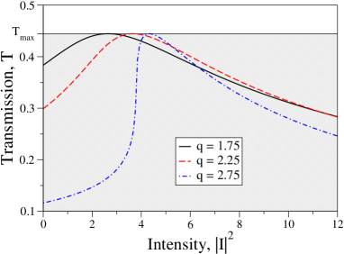
Figure 4: (Color online) Nonlinear transmission vs. intensity of the incoming wave $|I|^{2}$ for different values of the wave number $q$. Other parameters are: $N=3$, $\epsilon_{0}=-1$, and $\lambda=1$. The maximum transmission can be achieved for any value of the wave number $q$ by tuning the intensity $|I|^{2}$ of the incoming wave. The shaded area indicates the possible values of the transmission coefficient.

The presence of nonlinear junction generates much richer dynamics for the transmission. The transmission coefficient can now be written in the form,

$$T=\frac{4}{N^{2}}\frac{1}{(x^{2}+1)}\;,$$ (17)

where $x$ satisfies the cubic equation

$$(x^{2}+1)(x-\alpha_{q})-\gamma_{q}=0,$$ (18)

$\gamma_{q}=\lambda 4I^{2}/(N^{3}\sin q)$ is the normalized nonlinear parameter, and $c_{q}=2\sin q$. The maximum transmission $T_{\rm max}=4/N^{2}$ takes place when $x=0$ is a solution of Eq. (18), i.e., when $\alpha_{q}=-\gamma_{q}$. It implies that the maximum transmission can be achieved for any frequency by a proper tuning of the intensity of the incoming wave [Fig. 4]. Moreover, the analysis of the cubic equation (18) reveals that for $|\alpha_{q}|>\sqrt{3}$ three solutions are possible, and the bistable transmission should occur (Fig.5). We summarize all those scenarios in Fig. 6. We notice that the maximum transmission curve, $\gamma_{q}=-\alpha_{q}$, lies almost at the boundary of the bistability region.

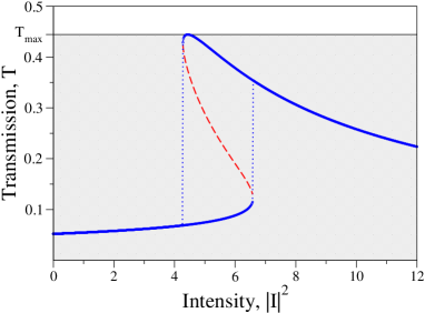
Figure 5: (Color online) Bistable nonlinear transmission in the nonlinear junction for $q=2.9$. Other parameters are the same as in Fig. 4. Bistability takes place near the maximum transmission. The shaded area indicates the possible values of the transmission coefficient.

V Results of numerical simulations

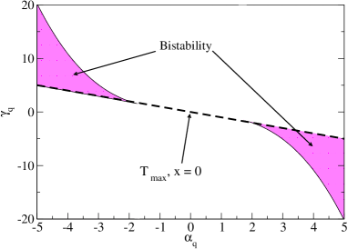
Figure 6: (Color online) Bistability diagram described by the solutions of the cubic equation (18). For the system parameters inside the shaded region there exist three solutions of the cubic equation, and the bistable nonlinear transmission should be observed (see Fig. 5). The solution $x=0$ corresponds to the maximum transmission $T_{\rm max}=4/N^{2}$, and it is shown as a dashed line $\gamma_{q}=-\alpha_{q}$.

In order to verify our theoretical results, we perform direct numerical simulations of the system (II) under more realistic pulse propagation. We launch a Gaussian pulse, along the branch $k=1$ and study numerically its propagation through the junction,

$$\phi_{n}^{(1)}(0)=I_{0}\exp\{-\frac{(n-n_{0})^{2}}{\sigma^{2}}-iq_{0}(n-n_{0})\}\;,$$ (19)

where $q_{0}$ is the pulse momentum, $I$ is the maximum amplitude of the wavepacket, $\sigma$ is the spatial width, and $n_{0}$ is the initial position.

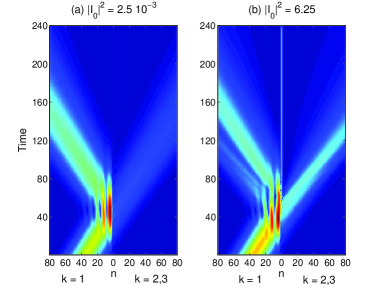
Figure 7: (Color online) Evolution of a Gaussian pulse scattered by the $N=3$ nonlinear junction (a nonlinear $Y$-splitter), for two different pulse intensities: (a) $|I|^{2}=2.5\times 10^{-3}$, and (b) $I=6.25$. Other parameters are: $\epsilon_{0}=-1$, $\lambda=1$, $\sigma=20$ and $q_{0}=2.75$. These results should be compared with the results for the plane-wave scattering shown in Fig. 4.

For our numerical simulations, we consider the case of a nonlinear $Y$-junction splitter ($N=3$) with $\epsilon_{0}=-1.$ and $\lambda=1.$ [see Fig. 4]. Figure 7 shows our results for the wave number $q_{0}=2.75$ for two different intensities of the Gaussian pulse. In this figure, we show the temporal pulse evolution in two branches only ($k=1$ and $k=2$) since, because of symmetry, the evolution in the branches $k=2$ and $k=3$ coincide.

because the evolution in the third branch $k=3$ coincides with that in the branch $k=2$ due to a symmetry.

When the pulse intensity is small [see Fig. 7(a)], the whole Gaussian pulse is reflected back into the incoming branch $k=1$, in agreement with our theoretical results [Fig. 4]. For larger values of the pulse intensity [see Fig. 7(b)], we observe an almost optimal splitting of the Gaussian pulse into the branches $k=2$ and $k=3$ with the maximum transmission [see Fig. 4]. We notice that in this case the junction $\phi_{0}$ remains highly excited even after the pulse already passed through it. The excitation of the nonlinear localized state at the junction is possible because of $\epsilon_{0}=-1$, one of the localized states interact strongly with the linear spectrum band (and its eigenvalue touches the band edge, see Fig. 2).

VI Conclusions

We have analyzed the linear and nonlinear transmission through a junction created by crossing of $N$ identical branches of a network of discrete linear waveguides. We have revealed that for $N>2$ such a junction behaves as an effective topological defect and supports two types of spatially localized linear modes. We have studied the transmission properties of this junction defect and demonstrated analytically that the reflection coefficient of the junction never vanishes, i.e. the wave scattering is always accompanied by some reflection. We have considered the case when the junction defect is nonlinear, and studied the nonlinear transmission of such a local nonlinear defect. We have demonstrated that nonlinearity allows achieving the maximum transmission for any frequency by tuning the intensity of the incoming wave but, in addition, the system can demonstrate bistability near the maximum transmission. We have confirmed our analytical results by direct numerical simulations.

References

- (1) M.I. Molina and G.P. Tsironis, Phys. Rev. B 47, 15330 (1993); M.I. Molina ibid. 71, 035404 (2005).
- (2) R. Burioni, D. Cassi, P. Sodano, A. Trombettoni, and A. Vezzani, Chaos 15, 043501 (2005).
- (3) R. Burioni, D. Cassi, P. Sodano, A. Trombettoni, and A. Vezzani, Phys. Rev. E 73, 066624 (2006).
- (4) M.I. Molina, Phys. Rev. B 67, 054202 (2003).
- (5) A.E. Miroshnichenko, S.F. Mingaleev, S. Flach, and Yu.S. Kivshar, Phys. Rev. E 71, 036626 (2005).
- (6) A.E. Miroshnichenko and Yu.S. Kivshar, Phys. Rev. E 72, 056611 (2005).
- (7) D.N. Christodoulides and E.D. Eugenieva, Opt. Lett. 26, 1876 (2001).
- (8) D.N. Christodoulides and E.D. Eugenieva, Phys. Rev. Lett. 87, 233901 (2001).
- (9) R. Burioni, D. Cassi, P. Sodano, A. Trombettoni, and A. Vezzani, Physica D216, 71 (2006).
- (10) S. Fan, P.R. Villeneuve, J.D. Joannopoulos, and H.A. Haus, Phys. Rev. Lett. 80, 960 (1998).
- (11) S.F. Mingaleev, A.E. Miroshnichenko, Yu.S. Kivshar, and K. Busch, Phys. Rev. E 74, 046603 (2006).
- (12) S. Pereira, P. Chak, and J.E. Sipe, J. Opt. Soc. Am. B 19, 2191 (2002).