Coarse-grained strain dynamics and backwards/forwards dispersion

Abstract

A Particle Tracking Velocimetry experiment has been performed in a turbulent flow at intermediate Reynolds number. We present experimentally obtained stretching rates for particle pairs in the inertial range. When compensated by a characteristic time scale for coarse-grained strain we observe constant stretching. This indicates that the process of material line stretching taking place in the viscous subrange has its counterpart in the inertial subrange. We investigate both forwards and backwards dispersion. We find a faster backwards stretching and relate it to the problem of relative dispersion and its time asymmetry.

I Introduction

The time asymmetry existing in a turbulent flow governed by the Navier-Stokes equation has recently been discussed in the connection with the diffusion properties of two nearby fluid particles initially close to each other. A stochastic model study by Sawford et al. (2005) showed that backwards dispersion is faster than the corresponding forwards dispersion. This has practical implications for a variety of applications dealing with transport and mixing in turbulent flows.

The asymmetry was experimentally verified by a Particle Tracking Velocimetry (PTV) experiment by Berg et al. (2006) who speculated that kinematic infinitesimal material line stretching has its counter-part in the inertial range. Different stretching rates could then explain the observed difference in forwards and backwards dispersion. Through a finite Reynolds number formulation of the much celebrated Richardson law $\langle r^{2}\rangle=g\varepsilon t^{3}$ it was found that following two particles backwards in time the dispersion was faster by a factor of approximately two compared with following the particles forwards in time. This ratio was also obtained from Direct Numerical Simulation (DNS) analysis by the same authors (data originally presented in (Biferale et al., 2004, 2005b)). Sawford et al. (2005) found the same ratio to be much larger: between $5$ and $20$.

Yet another stochastic model was developed by Lüthi et al. (2006). By assuming that stretching rates behave self-similar results consistent with Berg et al. (2006) were obtained. By self-similar stretching we think of particle separation which is similar on the different scales. The self-similarity of stretching rates has, however, not been shown.

In this paper we will explore forwards/backwards dispersion in the context of coarse-grained strain dynamics. The latter has recently got a lot of attention in the turbulence community since it is more or less related to Large Eddy Simulations (LES) (Borue and Orszag, 2002; Chertkov et al., 1999; Tao et al., 2002; van der Bos et al., 2002; Pumir and Shraiman, 2003; Naso et al., 2006; Lüthi et al., 2006). One can expect Kolmogorov similarity scaling to hold for the coarse-grained quantities as long as the filtering scale is less than the integral scale in the flow where the turbulence is solely represented by the kinetic energy dissipation of the flow, $\varepsilon$

As in Lüthi et al. (2006) we define the coarse-grained velocity gradient tensor to be

$$\widetilde{A}^{\Delta}_{ij}=\frac{\partial\widetilde{u}^{\Delta}_{j}}{\partial x_{i}},$$ (1)

where $\tilde{\mathbf{u}}^{\Delta}(\mathbf{x},t)$ is the coarse-grained velocity over scale $\Delta$:

$$\widetilde{u}^{\Delta}_{i}(\mathbf{x})=\frac{1}{V}\int_{B_{\Delta/2}}d\mathbf{r}\hskip 1.42271ptu_{i}(\mathbf{x}+\mathbf{r}).$$ (2)

Here $B_{\Delta/2}$ denotes a Ball with radius $\Delta/2$ and $V$ its volume.

We will follow the lines of Berg et al. (2006) and Lüthi et al. (2006) and present experimental evidence of self-similar stretching in a turbulent flow of intermediate Reynolds number. The result is linked to particle pair separation and is able to account for the difference in forwards and backwards dispersion.

II Experimental method

We have performed a Particle Tracking Velocimetry (PTV) experiment in an intermediate Reynolds number turbulent flow. The flow has earlier been reported in Berg et al. (2006). PTV is an experimental method suitable for obtaining Lagrangian statistics in turbulent flows (Ott and Mann, 2000; Porta et al., 2001; Mordant et al., 2001; Lüthi et al., 2005; Bourgoin et al., 2006; Xu et al., 2006): Lagrangian trajectories of fluid particles in water are obtained by tracking neutrally buoyant particles in space and time. The flow is generated by eight rotating propellers, which change their rotational direction in fixed intervals in order to suppress a mean flow, placed in the corners of a tank with dimensions $32\times 32\times 50\mathrm{cm}^{3}$ (see Fig 1).

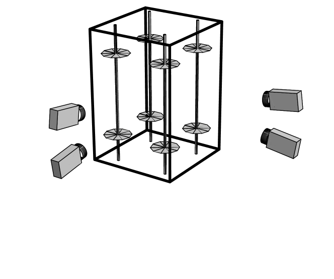
Figure 1: Experimental setup

The data acquisition system consists of four commercial CCD cameras with a maximum frame rate of $50\mathrm{Hz}$ at $1000\times 1000$ pixels. The measuring volume covers roughly $(12\mathrm{cm})^{3}$. We use polystyrene particles with size $\sim 400\mathrm{\mu m}$ and density very close to one. We follow $\mathcal{O}(1000)$ particles at each time step with a position accuracy of $0.05$ pixels corresponding to less than $10\mathrm{\mu m}.$

The Stokes number, $\tau_{I}/\tau_{\eta}$ ($\tau_{I}$ denotes the inertial relaxation time for the particle to the flow while $\tau_{\eta}$ is the Kolmogorov time) is much less than one and the particles can therefore be treated as passive tracers in the flow. The particles are illuminated by a $250\mathrm{W}$ flash lamp.

The mathematical algorithms for translating two dimensional image coordinates from the four camera chips into a full set of three dimensional trajectories in time involve several crucial steps: fitting gaussian profiles to the 2d images, stereo matching (line of sight crossings) with a two media (water-air) optical model and construction of 3d trajectories in time by using the kinematic principle of minimum change in acceleration (Willneff, 2003; Ouellette et al., 2006).

$\eta$	$L_{int}$	$\tau_{\eta}$	$T_{L}$	$\varepsilon$	$\sigma_{u}$	$Re_{\lambda}$
$0.25\mathrm{mm}$	$48\mathrm{mm}$	$0.07\mathrm{s}$	$2.45\mathrm{s}$	$168\mathrm{mm^{2}/s^{3}}$	$23.33\mathrm{mm/s}$	172

Table 1: Turbulence characteristics obtained from the von Kármán model Ott and Mann (2000): Mean kinetic energy dissipation $\varepsilon$, Kolmogorov length $\eta\equiv(\nu^{3}/\varepsilon)^{1/4}$, Kolmogorov time $\tau_{\eta}\equiv(\nu/\varepsilon)^{1/2}$, integral length $L_{int}$, integral time $T_{L}$, velocity fluctuations $\sigma_{u}^{2}=\frac{1}{3}(\sigma_{u_{x}}^{2}+\sigma_{u_{y}}^{2}+\sigma_{u_{z}}^{2}).$ The Reynolds number is defined as $Re_{\lambda}=\frac{\lambda\sigma_{u}}{\nu}$ with the Taylor micro scale $\lambda=\sqrt{\left(\frac{15\nu\sigma^{2}}{\varepsilon}\right)}.$

From eqn. 1 we can define the coarse grained strain $\langle\widetilde{s}^{2}\rangle$ and $\langle\widetilde{\Omega}^{2}\rangle$ where $\langle\widetilde{s}_{ij}\rangle$ and $\langle\widetilde{\Omega}_{ij}\rangle$ are the symmetric and anti-symmetric part of the coarse-grained velocity gradient tensor $\langle\widetilde{A}_{ij}\rangle$. The eigenvalues and eigenvector of $\langle\widetilde{s}_{ij}\rangle$ is denoted $\langle\widetilde{\Lambda}_{i}\rangle$ and $\langle\widetilde{\lambda}_{i}\rangle$ respectively. Due to incompressibility $\sum_{i}\langle\widetilde{\Lambda}_{i}\rangle=0$. In addition we define $\langle\widetilde{\Lambda}_{1}\rangle>\langle\widetilde{\Lambda}_{2}\rangle>\langle\widetilde{\Lambda}_{3}\rangle$ so that the most positive principal direction of strain is $\langle\widetilde{\Lambda}_{1}\rangle$.

The filtered velocity field (eqn. 2) is approximated by least square fits of spherical incompressible and orthogonal linear polynomials to discrete velocities of fluid particles inside spherical balls with diameter $\Delta$:

$$\min\left[\int_{B(\Delta/2)}d^{3}\mathbf{x}\hskip 2.84544pt(u_{i}-\widetilde{A}_{ij}x_{j})^{2}\right]$$ (3)

At least four particles are necessary to describe a three-dimensional shape and hence to estimate $\langle\widetilde{A}_{ij}\rangle.$ Four particles form a tetrahedron and is the backbone of the analysis by Chertkov et al. (1999). In Lüthi et al. (2006) we show that $\widetilde{A}_{ij}$ obtained from only four particles is quite far from the definition in eqn. 2 and therefore that using only four particles are not sufficient.

We find that at least twelve particles are needed in order to obtain a reasonable approximation of eqn. 2 of the coarse-grained quantities. Using this many particles has the drawback that we can not study the dynamics at the smallest scales. In Figure 2 (a) the radial distribution of particles is shown. The probability $Np(r)$ of finding a given number $N$ of particles on the surface of a ball centered in our measuring volume with radius $r$ is observed to increase with $r^{2}$ up to $\sim 200\eta$. This means that the particle density can be considered uniform up to this scale. For lager radius the density drops down because of non-perfect illumination at the boundary of the measuring volume. The cumulative distribution is show in (b) and is interesting because it gives us an estimate of the number of particles we can expect to find in a ball with radius $r$. The number is, however, only an upper bound since the ball is centered in the measuring volume and not around all individual particles in the flow.

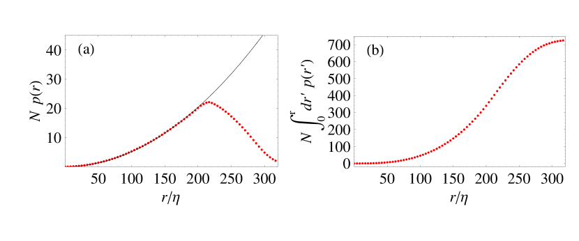
Figure 2: Radial distribution of particles where $N$ is the total number of particles in the volume. a) The probability of finding a particle in a spherical shell with thickness $dr$ and with distance $r$ from the center of the measuring volume. b) Cumulative distribution of (a).

The smallest scale for which $\langle\widetilde{u}\rangle$ and hence $\langle\widetilde{s}^{2}\rangle$ and $\langle\widetilde{\Omega}^{2}\rangle$ can be resolved is $80\eta.$ A higher particle seeding density which again makes particle tracking more difficult can decrease this number. All results reported use a minimum of twelve particles.

As already reported in Berg et al. (2006); Lüthi et al. (2006) the mean flow is slightly straining though with a characteristic time scale many times larger than the integral time scale of the flow. An alternative way of emphasizing the large scale mean strain is shown in Figure 3. $\cos^{2}(x_{i},\widetilde{\lambda}_{1}),$ where $x_{i}$ is the three coordinate axes, is observed to peak for large $r$ in the vertical direction while the horizontal axes decrease in agreement with an axis-symmetric flow. A slow convergence towards isotropy is observed as $r=\Delta$ is reduced.

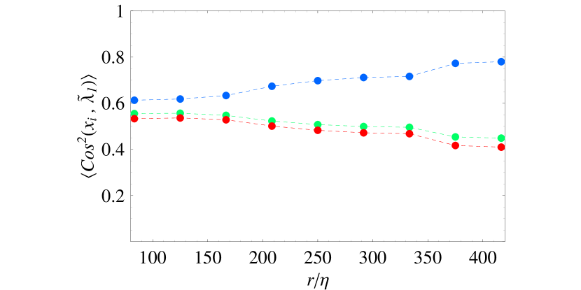
Figure 3: Squared cosine between the most stretching principle coarse grained eigenvector, $\widetilde{\lambda}_{1}$, and the three coordinate directions. Blue is the vertical axis-symmetric direction while the green and red is the horizontal directions.

III Coarse-grained statistics

In the viscous subrange the stretching rate of infinitesimal material lines governs particle pair separation. The stretching rate is defined as

$$L(t)=\left\langle\frac{1}{2r^{2}}\frac{dr^{2}}{dt}\right\rangle.$$ (4)

where $d/dt$ denotes Lagrangian differentiation (following the particles). In the viscous subrange $L(t)$ when rescaled with the Kolmogorov time scale $\tau_{\eta}$ becomes constant after a short time (Biferale et al., 2005a; Girimaji and Pope, 1990; Guala et al., 2005; Berg et al., 2006; Lüthi et al., 2005). In the viscous sub range the second order Eulerian longitudinal structure function $f(r)=\langle\{[u_{i}(\mathbf{x}+\mathbf{r})-u_{i}(\mathbf{x})]r_{i}/r\}^{2}\rangle$ is given by

$$f(r)=\frac{\langle s^{2}\rangle}{15}r^{2}\hskip 28.45274ptr\ll\eta$$ (5)

Through the definitions $\varepsilon=2\nu\langle s^{2}\rangle$ and $\tau_{\eta}^{2}=\nu/\varepsilon$ we can form $\tau_{\eta}^{2}=r^{2}/(30f(r)).$ Thus motivated by viscous subrange scaling we move to the inertial range and define a time scale

$$t_{\star}(r)=\sqrt{\frac{2r^{2}}{15f(r)}}\hskip 28.45274ptr\ll L_{int}.$$ (6)

In the limit $r\ll\eta$ we have $t_{\star}=\sqrt{2}\tau_{\eta}$.

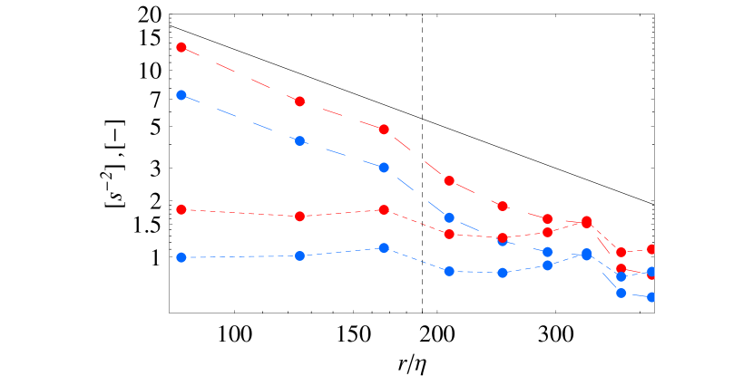
Figure 4: Coarse grained strain $\langle\widetilde{s}^{2}\rangle$ (long dashed blue) and $\langle\widetilde{\Omega}^{2}\rangle$ (long dashed red) as a function of coarse graining scale $r.$ The solid black line is $r^{-4/3}$. The dotted lines are $\langle\widetilde{s}^{2}\rangle$ and $\langle\widetilde{\Omega}^{2}\rangle$ multiplied by $t_{\star}^{2}.$ The vertical black dotted line indicates the integral length scale.

As a function of scale $r=\Delta$ we plot $\langle\widetilde{s}^{2}\rangle$ and $\langle\tilde{\Omega}^{2}\rangle$ in Figure 4. Both quantities are in the inertial range observed to be in agreement with the Kolmogorov similarity prediction $r^{-4/3}.$ For $r\rightarrow 0$ the ratio $\langle\widetilde{\Omega}^{2}\rangle/\langle\tilde{s}^{2}\rangle\rightarrow 2$.

Also in Figure 4 we have plotted $\langle\widetilde{s}^{2}\rangle$ and $\langle\widetilde{\Omega}^{2}\rangle$ multiplied with $t^{2}_{\star}$. In the inertial range we find that $\langle\widetilde{s}^{2}\rangle t^{2}_{\star}\sim 1$ and $\langle\widetilde{\Omega}^{2}\rangle t^{2}_{\star}=1.85.$ It thus seems that $t_{\star}$ as defined in eqn. 6 serves as a characteristic time scale for $\langle\widetilde{s}^{2}\rangle$ and therefore $t_{\star}\sim 1/\sqrt{\langle\widetilde{s}^{2}\rangle}$.

In Lüthi et al. (2006) $f(r)$ in eqn. 6 was defined through a model valid for homogeneous and isotropic turbulence. In this paper $f(r)$ are obtained directly from data. The behavior therefore is therefore slightly different.

IV Particle pair separation

The rescaled eigenvalues $\langle\widetilde{\Lambda}_{i}\rangle t_{\star}$ are shown in Figure 5. The trademark of turbulence, namely $\langle\widetilde{\Lambda}_{2}\rangle>0$ which is necessary for both positive mean enstrophy and strain production is observed for all values of $r$. A slight decrease in $\langle\widetilde{\Lambda}_{2}\rangle$ is observed as $r$ is increased which could be taken as a sign of the coarse-graining field becoming more Gaussian and hence $\langle\widetilde{\Lambda}_{2}\rangle=0.$ Both $\langle\widetilde{\Lambda}_{1}\rangle t_{\star}$ and $\langle\widetilde{\Lambda}_{3}\rangle t_{\star}$ are constant and so are their ratio $|\langle\widetilde{\Lambda}_{3}\rangle|/|\langle\widetilde{\Lambda}_{1}\rangle|$. For a direct comparison with viscous result we have divided the results with $\sqrt{2}$.

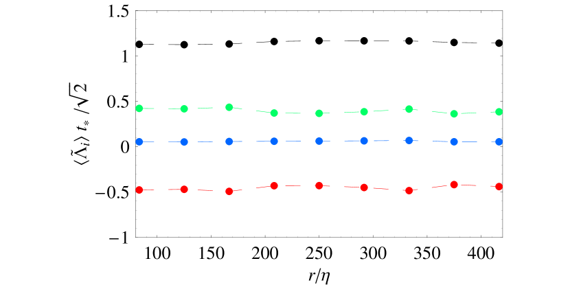
Figure 5: Eigenvalues $\langle\widetilde{\Lambda}_{i}\rangle t_{\star}$ of $\langle\widetilde{s}_{ij}\rangle$. $i=1$: green, $i=2$: blue and $i=3$: red. The black curve is the ratio $|\langle\widetilde{\Lambda}_{3}\rangle|/|\langle\widetilde{\Lambda}_{1}\rangle|$.

When time is running forward two particles in a mean strain field will on average separate from each other along the direction of $\langle\widetilde{\lambda}_{1}\rangle$. In the backward case they will separate along the direction of $\langle\widetilde{\lambda}_{3}\rangle$. Since $\langle\widetilde{\Lambda}_{2}\rangle>0$ and therefore $|\langle\widetilde{\Lambda}_{3}\rangle|>|\langle\widetilde{\Lambda}_{1}\rangle|$ backwards separation is the faster one. This is shown in Figure 6 for times $t_{B}<t<5t_{B}$ where $t_{B}=(r^{2}_{0}/\varepsilon)^{1/3}$ is the Batchelor time, characterizing the time for which the initial separation should be regarded an important parameter in the separation process Bourgoin et al. (2006).

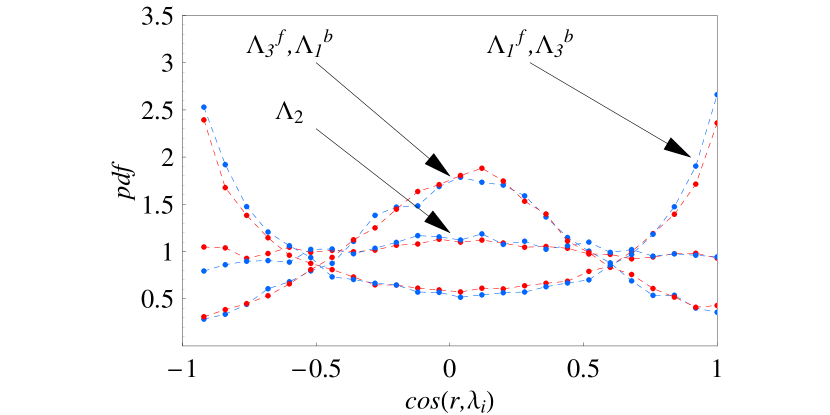
Figure 6: Angular dependence between $\langle\widetilde{\lambda_{i}}\rangle$ and the separation vector $r$ for times $t_{B}\gg t\gg 5t_{B}$. Red curves are forwards dispersion while blue are backwards dispersion.

By closer inspection of Figure 6 we can see that in the backward case $r$ is slightly more aligned with $\langle\widetilde{\lambda}_{3}\rangle$ than it is aligned with $\langle\widetilde{\lambda}_{1}\rangle$ in the forward case. This is due to the positiveness of $\langle\widetilde{\Lambda}_{2}\rangle$ and a corresponding increase in the alignment of $r$ with $\langle\widetilde{\lambda}_{2}\rangle$ in the forward case compared to in the backward case is therefore also observed. The values of $\cos^{2}{(r,\widetilde{\lambda}_{i})}$ are in the forward case $0.50$, $0.32$ and $0.19$ for $i=1,2,3$ respectively. In the backward case the same values are $0.19$, $0.28$ and $0.53$.

Stretching rates rescaled by $t_{\star}$ are presented in Figure 7 as a function of $t/t_{B}$ for different initial separation of pairs.

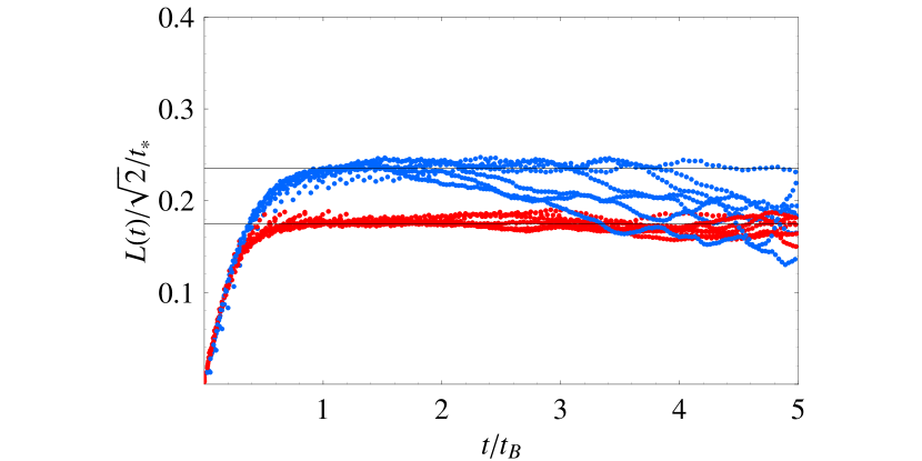
Figure 7: Stretching rates $L(t)$ rescaled by $t_{\star}$. The blue curves correspond to forwards separation while the red curves corresponds to backwards separation (time running backwards) for different initial separations $r_{0}$. Particle pairs with $r_{0}$ from $3-4\mathrm{mm}$ to $9-10\mathrm{mm}$ in steps of $1mm$ are shown. We have divided the $y$-axis with $\sqrt{2}$ in order to match the viscous limit.

For times $t\sim 0.5t_{B}$ the forward stretching and backward stretching occurs with the same speed. The separation vector is still randomly oriented and has therefore not yet aligned itself with the principal directions of the strain field. For longer times the backwards stretching rates saturates at $0.235\pm 0.005$ while the forwards saturate at $0.18\pm 0.005$. Whereas all curves in the forward case collapse for times up to $3-4t_{B}$ the curves in the backward case do not collapse so nicely. Because backward separation is faster the particles leave the measurement volume earlier: the larger $r_{0}$, the earlier. The particle pairs we thus observe for large times are likely to be slow pairs with low stretching rate. To reduce the effect of finite volume we only choose pairs which start within a small sub volume ($30\mathrm{mm}$) of the full measuring volume. There is, however, no systematic way in which we can totally neglect the effect of a finite volume.

The maximum stretching rates would occur if the particle separation vector $\mathbf{r}$ is fully aligned with the principal strain axes. In this case the rescaled stretching rates would be $\langle\widetilde{\Lambda}_{1}\rangle t_{\star}$ and $-\langle\widetilde{\Lambda}_{3}\rangle t_{\star}$ in Figure 5 for the forward and backward case respectively. The forward value $L_{f}(t)/\sqrt{2}/t_{\star}=0.18\pm 0.005$ is close to the values obtained in the viscous sub range Biferale et al. (2005a); Girimaji and Pope (1990); Guala et al. (2005); Berg et al. (2006).

Berg et al. (2006) hypothesized that, if the particle separation was perfectly aligned with the principal strain axes, the ratio between forwards and backwards dispersion rates characterized by the Richardson-Obukhov constant ratio $g_{b}/g_{f}$ could be determined as $|\langle\widetilde{\Lambda}_{3}\rangle|/\langle\widetilde{\Lambda}_{1}\rangle)^{3}$. From Figure 5 this number equals $1.13^{3}=1.44$. From the calculated stretching rates we find that this is certainly not the case since $0.235/0.18=1.31$. With the same argumentation this would give a ratio $g_{b}/g_{f}=2.23\pm 0.33$ within errors of what was measured directly in Berg et al. (2006). Although $L(t)_{f}\leq|\langle\widetilde{\Lambda}_{1}\rangle|$ and $L(t)_{b}\leq|\langle\widetilde{\Lambda}_{3}\rangle|$ we thus have $L(t)_{b}/L(t)_{f}\leq|\langle\widetilde{\Lambda}_{3}\rangle/\langle\widetilde{\Lambda}_{1}\rangle|$ and hence a larger ratio than in the fully aligned case. It is important to stress that the argumentation of how to relate the ratio $g_{b}/g_{f}$ to $L(t)_{b}/L(t)_{f}$ through the Richardson-Obukhov law is not a rigourously derived result but merely a hand waving argument.

V Conclusions

We have given evidence of the existence of, what we call self-similar stretching rates: when scaled by a relevant time $t_{\star}$ scale which is a function of the second order structure function stretching rates of infinitesimal material lines has its counterpart in the inertial range. Furthermore it turns out that this relevant time scale $t_{\star}$ is related to the coarse-grained strain field. The stretching is like in the viscous range far from being perfectly aligned with the most positive direction of strain which we have shown would lower the ratio between forwards and backwards dispersion.

Whether or not the Lagrangian stretching rates found in this paper are universal or specific for this particular turbulent flow other experiments and/or DNS will have to decide.

References

- Berg et al. [2006] J. Berg, B. Lüthi, J. Mann, and S. Ott. Backwards and forwards relative dispersion in turbulent flow: An experimental investigation. Phys. Rev. E, 34:115, 2006.
- Biferale et al. [2004] L. Biferale, G. Boffetta, A. Celani, B. J. Devenish, A. Lanotte, and F. Toschi. Multifractal statistics of lagrangian velocity and acceleration in turbulence. Phys. Rev. Lett., 93:064502, 2004.
- Biferale et al. [2005a] L. Biferale, G. Boffetta, A. Celani, B. J. Devenish, A. Lanotte, and F. Toschi. Lagrangian statistics of particle pairs in homogeneous isotropic turbulence. Phys. Fluids, 17:115101, 2005a.
- Biferale et al. [2005b] L. Biferale, G. Boffetta, A. Celani, B. J. Devenish, A. Lanotte, and F. Toschi. Particle trapping in three-dimensional fully developed turbulence. Phys. Fluids, 17:021701, 2005b.
- Borue and Orszag [2002] V. Borue and S. A. Orszag. Local energy flux and subgrid scale statistics in three-dimensional turbulence. J. Fluid Mech., 366:1, 2002.
- Bourgoin et al. [2006] M. Bourgoin, N. T. Ouellette, H. Xu, J. Berg, and E. Bodenschatz. The role of pair dispersion in turbulent flow. Science, 311:835, 2006.
- Chertkov et al. [1999] M. Chertkov, A. Pumir, and B. I. Shraiman. Lagrangian tetrad dynamics and the phenomenology of turbulence. Phys. Fluids, 11:2394, 1999.
- Girimaji and Pope [1990] S. S. Girimaji and S. B. Pope. Material-element deformation in isotropic turbulence. J. Fluid Mech., 220:427, 1990.
- Guala et al. [2005] M. Guala, B. Lüthi, A. Liberzon, A. Tsinober, and W. Kinzelbach. On the evolution of material lines and vorticity in homogeneous turbulence. J. Fluid Mech., 533:339, 2005.
- Lüthi et al. [2006] B. Lüthi, J. Berg, S. Ott, and Mann J. Lagrangian multi-particle statistics. submitted, 2006.
- Lüthi et al. [2005] B. Lüthi, A. Tsinober, and W. Kinzelbach. Lagrangian measurements of vorticity dynamics in tubulent flow. J. Fluid Mech., 528:87, 2005.
- Mordant et al. [2001] N. Mordant, P. Metz, O. Michel, and J.-F. Pinton. Mearesurement of lagrangian velocity in fully developed turbulence. Phys. Rev. Lett., 87:214501, 2001.
- Naso et al. [2006] A. Naso, M. Chertkov, and A. Pumir. Scale dependence of the coarse-grained velocity derivative tensor: influence of large-scale shear on small-scale turbulence. J. turbulence, 7:41, 2006.
- Ott and Mann [2000] S. Ott and J. Mann. An experimental investigation of the relative diffusion of particle pairs in three-dimensional flow. J. Fluid Mech., 422:207, 2000.
- Ouellette et al. [2006] N. T. Ouellette, H. Xu, and E. Bodenschatz. A quantitative study of three-dimensional lagrangian particle tracking algorithms. Exp. in Fluids., 40:301, 2006.
- Porta et al. [2001] A. La Porta, G. A. Voth, J. Alexander A. M. Crawford, and E. Bodenschatz. Fluid particle accelerations in fully developed turbulence. Nature, 409:1017, 2001.
- Pumir and Shraiman [2003] A. Pumir and B. I. Shraiman. Lagrangian particle approach to large eddy simulations of hydrodynamic turbulence. J. Stat. Phys., 113:693, 2003.
- Sawford et al. [2005] B. L. Sawford, P. K. Yeung, and M. S. Borgas. Comparison of backwards and forwards relative dispersion in turbulence. Phys. Fluids, 17:095109, 2005.
- Tao et al. [2002] B. Tao, J. Katz, and C. Meneveau. Statistical geometry of subgrid-scale stresses determined from holographic particle image velocimetry measurements. J. Fluid Mech., 457:35, 2002.
- van der Bos et al. [2002] F. van der Bos, B. Tao, and J. Katz C. Meneveau and. Effects of small-scale turbulent motions on the altered velocity gradient tensor as deduced from holographic particle image velocimetry measurements. Phys. Fluids, 14:2456, 2002.
- Willneff [2003] J. Willneff. A spatio-temporal mathing algorithm for 3D-particle tracking velocimetry. PhD thesis, ETH Zürich, 2003.
- Xu et al. [2006] H. Xu, M. Bourgoin, N. T. Ouellette, and E. Bodenschatz. High order lagrangian velocity statistics in turbulence. Phys. Rev. Lett., 96:024503, 2006.