Reciprocal transmittances and reflectances: An elementary proof

Abstract

We present an elementary proof concerning reciprocal transmittances and reflectances. The proof is direct, simple, and valid for the diverse objects that can be absorptive and induce diffraction and scattering, as long as the objects respond linearly and locally to electromagnetic waves. The proof enables students who understand the basics of classical electromagnetics to grasp the physical basis of reciprocal optical responses. In addition, we show an example to demonstrate reciprocal response numerically and experimentally.

I Introduction

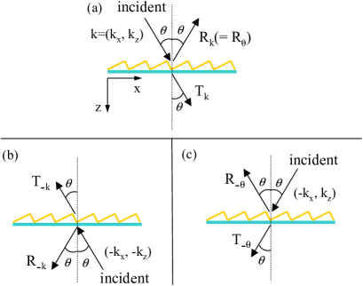
Figure 1: Reciprocal configurations. (a) and (b) show reciprocal configurations for transmission. $T_{\rm k}$ in (a) denotes transmittance for incident wavenumber vector ${\bf k}$. $T_{\rm-k}$ in (b) is defined similarly. The reciprocal relation is $T_{\rm k}=T_{\rm-k}$. (a) and (c) are reciprocal for reflection. $R_{\theta}$ in (a) is reflectance for incident wavenumber vector $(k_{x},k_{z})$ and $R_{-\theta}$ in (c) for $(-k_{x},k_{z})$. The reciprocal relation is $R_{\theta}=R_{-\theta}$.

Reciprocity, which was first found by Lorentz at the end of 19th century, has a long historyPotton and has been derived in several formalisms. There are two typical reciprocal configurations in optical responses as shown in Fig. 1. The configurations in Figs. 1(a) and 1(b) are transmission reciprocal and those in Figs. 1(a) and 1(c) are reflection reciprocal. As shown in Fig. 1, we denote transmittance by $T$ and reflectance by $R$; the suffice k and $\theta$ stand for incident wavenumber vector and angle, respectively. The reciprocal configurations are obtained by symmetry operations on the incident light of the wavenumber vector: ($k_{x},\,k_{z})\to(-k_{x},-k_{z}$) or ($-k_{x},\,k_{z}$). Reciprocity on transmission means that $T_{\rm k}=T_{\rm-k}$, and that on reflection is expressed as $R_{\theta}=R_{-\theta}$, which is not intuitively obvious and is frequently surprising to students.

The most general proof was published by Petit in 1980,Petit where reciprocal reflection as shown in Fig. 1 is derived for asymmetric gratings such as an echelette grating. On the basis of the reciprocal relation for the solutions of the Helmholtz equation, the proof showed that reciprocal reflection holds for periodic objects irrespective of absorption. It seems difficult to apply the proof to transmission because it would be necessary to construct solutions of Maxwell equations that satisfy the boundary conditions at the interfaces of the incident, grating, and transmitted layers. The history of the literature on reciprocal optical responses has been reviewed in Ref Potton, .

Since the 1950s, scattering problems regarding light, elementary particles, and so on have been addressed by using scattering matrix (S-matrix). In the studies employing the S-matrix, it is assumed that there is no absorption by the object. The assumption leads to the unitarity of the S-matrix and makes it possible to prove reciprocity. The reciprocal reflection of lossless objects was verified in this formalism.Gippius

In this paper we present a simple, direct, and general derivation of the reciprocal optical responses for transmission and reflection relying only on classical electrodynamics. We start from the reciprocal theorem described in Sec. II and derive the equation for zeroth order transmission and reflection coefficients in Sec. III. The equation is essential to the reciprocity. A numerical and experimental example of reciprocity is presented in Sec. IV. The limitation and break down of reciprocal optical responses are also discussed.

II Reciprocal Theorem

The reciprocal theorem has been proved in various fields, such as statistical mechanics, quantum mechanics, and electromagnetism.Landau Here we introduce the theorem for electromagnetism.

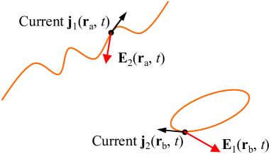
Figure 2: Schematic drawing of two currents ${\bf j}_{i}$ and the electric fields ${\bf E}_{i}$ induced by ${\bf j}_{i}$ ($i=1,2$). The curves denote the position where the currents exist.

When two currents exist as in Fig. 2 and the induced electromagnetic (EM) waves travel in linear and locally responding media in which $D_{i}({\bf r})=\sum_{j}\varepsilon_{ij}E_{j}({\bf r})$ and $B_{i}({\bf r})=\sum_{j}\mu_{ij}H_{j}({\bf r})$, then

$$\int{\bf j}_{1}({\bf r})\cdot{\bf E}_{2}({\bf r})d{\bf r}=\!\int{\bf j}_{2}({\bf r})\cdot{\bf E}_{1}({\bf r})d{\bf r}.$$ (1)

Equation (1) is the reciprocal theorem in electromagnetism. The proof shown in Ref. Landau, exploits plane waves and is straightforward. Equation (1) is valid even for media with losses. The integrands take non-zero values at the position ${\bf r}$ where currents exist, that is, ${\bf j}_{i}({\bf r})\neq{\bf 0}$. The theorem indicates the reciprocity between the two current sources ${\bf j}_{i}$ ($i=1,2$) and the induced EM waves ${\bf E}_{i}$ which are observed at the position of the other source ${\bf j}_{k}$ ($k\neq i$).

III Reciprocal Optical Responses

In this section, we apply the reciprocal theorem to optical responses in both transmission and reflection configurations. First, we define the notation used in the calculations of the integrals in Eq. (1). An electric dipole oscillating at the frequency $\omega$ emits dipole radiation, which is detected in the far field. When a small dipole ${\bf p}$ along the $z$ axis is located at the origin, it is written as ${\bf p}(t)=p(t){\bf e}_{z}$ and $p(t)=p_{0}e^{i\omega t}$, where ${\bf e}_{z}$ denotes the unit vector along the $z$ axis and $p_{0}$ the magnitude of the dipole. The dipole in vacuum emits radiation, which in the far field is

$${\bf E}({\bf r},t) =\frac{1}{4\pi\varepsilon_{0}}\frac{\ddot{p}(t^{\prime})}{c^{2}r}\sin\theta\cdot{\bf e}_{\theta}$$ (2a)

$$=\frac{-1}{4\pi\varepsilon_{0}}\frac{p_{0}\,\omega^{2}}{c^{2}r}e^{i\omega t^{\prime}}\sin\theta\cdot{\bf e}_{\theta},$$ (2b)

where polar coordinates ($r$, $\theta$, $\phi$) are used, a unit vector is given by ${\bf e}_{\theta}=(\cos\theta\cos\phi,\cos\theta\sin\phi,-\sin\theta)$, and $t^{\prime}=t-r/c$. Because the dipole ${\bf p}$ is defined by ${\bf p}({\bf r},t)=\!\int{\bf r}\rho({\bf r},t)d{\bf r}$ and conservation of charge density is given by $\nabla\cdot{\bf j}+\partial\rho/\partial t=0$, we obtain the current ${\bf j}$ associated with the dipole ${\bf p}$:

$${\bf j}({\bf r},t)=\dot{p}(t)\delta({\bf r}){\bf e}_{z}.$$ (3)

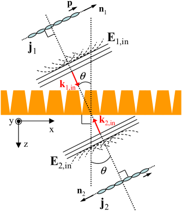
Figure 3: Schematic drawing of reciprocal configuration for transmission. The object has an arbitrary periodic structure, which is asymmetric along the $z$ axis. Currents ${\bf j}_{i}$ induce electric fields ${\bf E}_{i,{\rm in}}$ ($i=1,2$).

Consider two arrays of $N$ dipoles (long but finite) in the $xz$ plane as shown in Fig. 3. The two arrays have the same length, and the directions are specified by normalized vectors ${\bf n}_{i}$ ($i=1,2$) and ${\bf n}_{1}\parallel{\bf n}_{2}$. In this case, the current is ${\bf j}_{i}\parallel{\bf n}_{i}$. If the dipoles coherently oscillate with the same phase, then the emitted electric fields are superimposed and form a wave front at a position far from the array in the $xz$ plane as drawn in Fig. 3. The electric field vector of the wave front, ${\bf E}_{i,{\rm in}}$, satisfies ${\bf E}_{i,{\rm in}}\parallel{\bf n}_{i}$ and travels with wavenumber vector ${\bf k}_{i,{\rm in}}$. Thus, if we place the dipole arrays far enough from the object, the induced EM waves become slowly decaying incident plane waves in the $xz$ plane to a good approximation. The arrays of dipoles have to be long enough to form the plane wave.

For the transmission configuration, we calculate $\int{\bf j}_{i}\cdot{\bf E}_{k}\,d{\bf r}$ ($i,k=1,2$ and $i\neq k$). Figure 3 shows a typical transmission configuration, which includes an arbitrary periodic object asymmetric along the $z$ axis. The relation between the current ${\bf j}_{i}$, the direction ${\bf n}_{i}$ of the dipole, and the wavenumber vector ${\bf k}_{i,{\rm in}}$ of the wave front is summarized as ${\bf j}_{i}\parallel{\bf n}_{i}$ and ${\bf n}_{i}\perp{\bf k}_{i,{\rm in}}$. It is convenient to expand the electric field into a Fourier series for the calculation of periodic sources:

$${\bf E}({\bf r})=\sum_{m}{\bf E}^{(m)}\exp(i{\bf k}_{m}\cdot{\bf r}),$$ (4)

where ${\bf E}^{(m)}$ is the Fourier coefficient of ${\bf E}({\bf r})$, ${\bf k}_{m}=(k_{x,m},0,k_{z,m})=(k_{{\rm in},x}+2\pi m/d_{x},0,k_{z,m})$ ($m=0,\pm 1,\pm 2,\cdots$), and $d_{x}$ is the periodicity of the object along the $x$ axis (see Fig. 3). The $z$ component is expressed in homogeneous media in vacuum as $k_{z,m}=\pm\sqrt{{\bf k}_{\rm in}^{2}-k_{x,m}^{2}}$, where the signs correspond to the directions along the $z$ axis.

When the dipole array is composed of sufficiently small and numerous dipoles, the integration can be calculated to good accuracy as

$$\int{\bf j}_{1}({\bf r})\cdot{\bf E}_{2}({\bf r})d{\bf r} =\!\int i\omega p_{0}{\bf n}_{1}\cdot\sum_{m}{\bf E}_{2}^{(m)}\exp(i{\bf k}_{m}\cdot s{\bf n}_{1})ds$$ (5a)

$$=\sum_{m}\delta_{m,0}N(i\omega p_{0}{\bf n}_{1}\cdot{\bf E}_{2}^{(m)})$$ (5b)

$$=i\omega Np_{0}E_{2}^{(0)},$$ (5c)

where $E_{2}^{(0)}=|{\bf E}_{2}^{(0)}|$. To ensure that the integration is proportional to $\delta_{m,0}$, the array of dipoles has to be longer than $L$:

$$L=(\mbox{length of dipole})\cdot q,$$ (6)

where $q$ is the least common multiple of the diffraction channels which are open at the frequency $\omega$. This condition would usually be satisfied when ${\bf E}_{i,{\rm in}}$ forms a plane wave.

By permutating 1 and 2 in Eq. (5c), we obtain $\int{\bf j}_{2}\cdot{\bf E}_{1}d{\bf r}=i\omega Np_{0}E_{1}^{(0)}$. Equation (5c) and the reciprocal theorem in Eq. (1) lead to the equation

$$E_{1}^{(0)}=E_{2}^{(0)}.$$ (7)

Each electric vector $E_{i}^{(0)}$ ($i=1,2$) is observed at the position ${\bf r}$ where there is another current ${\bf j}_{k}({\bf r})$ ($k\neq i$). The integral in Eq. (1) is reduced to Eq. (5c) which is expressed only by the zeroth components of the transmitted electric field. The reciprocity is thus independent of higher order harmonics, which are responsible for the modulated EM fields in structured objects. When there is no periodic object in Fig. 3, a similar relation holds:

$$E_{1}^{\rm no,(0)}=E_{2}^{\rm no,(0)}.$$ (8)

The transmittance $T_{i}$ is given by

$$T_{i}=\left|\frac{E_{i}^{(0)}}{E_{i}^{\rm no,(0)}}\right|^{2}.$$ (9)

From Eqs. (7)–(9), we finally reach the reciprocal relation $T_{1}=T_{2}$.

The feature of the proof that $T_{1}=T_{2}$ is independent of the detailed evaluation of $E_{i}^{(0)}$ and therefore makes the proof simple and general. The proof can be extended to two-dimensional periodic structure by replacing the one-dimensional periodic structure in Fig. 3 by two-dimensional one. Although we have considered periodic objects, the proof can also be extended to non-periodic objects. To do this extension, Eq. (4) has to be expressed in the general form ${\bf E}({\bf r})=\int{\bf E}({\bf k})\exp(i{\bf k}\cdot{\bf r})d{\bf k}$, and a more detailed calculation for $\int{\bf j}_{i}\cdot{\bf E}_{k}d{\bf r}$ is required. Reciprocity for transmission thus holds irrespective of absorption, diffraction, and scattering by objects.

In Fig. 3 the induced electric fields ${\bf E}_{i}$ are polarized in the $xz$ plane. The polarization is called TM polarization in the terminology of waveguide theory and is also often called $p$ polarization. For TE polarization (which is often called $s$ polarization) for which ${\bf E}_{i}$ has a polarization parallel to the $y$ axis, the proof is similar to what we have described except that the dipoles are aligned along the $y$ axis.

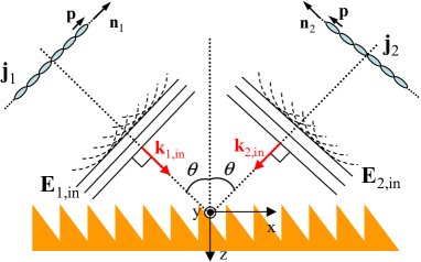
Figure 4: Schematic configuration for reciprocal reflection. The object has an arbitrary periodic structure, which consists of asymmetric unit cells. The currents ${\bf j}_{i}$ yield electric fields ${\bf E}_{i,{\rm in}}$ ($i=1,2$).

Reciprocal reflection is also shown in a similar way. The configuration is depicted in Fig. 4. The two sources have to be located to satisfy the mirror symmetry about the $z$ axis. The calculation of $\int{\bf j}_{i}\cdot{\bf E}_{k}d{\bf r}$ leads to the reciprocal relation for reflectance $R_{1}=R_{2}$. Note that $E_{i}^{{\rm no},(0)}$ in Eq. (8) has to be evaluated by replacing the periodic object by a perfect mirror.

IV Numerical and Experimental Confirmation

An example of reciprocal optical response is shown here. Figure 5(a) displays the structure of the sample and reciprocal transmission configuration. The sample consists of periodic grooves etched in metallic films of Au and Cr on a quartz substrate. The periodicity is 1200 nm, as indicated by the dotted lines in Fig. 5(a). The unit cell has the structure of Au:air:Au:air = 3:1:4:5. The thickness of Au, Cr, and quartz is 40 nm, 5 nm, and 1 mm, respectively. The structure is obviously asymmetric about the $z$ axis. The profile was modeled from an AFM image of the fabricated sample.

Figure 5(b) shows our numerical results. The incident light has $\theta=10^{\circ}$ and TM polarization (the electric vector is in the $xz$ plane). The numerical calculation was done with an improved S-matrix methodTikh ; Li1 The permittivities of gold and chromium were taken from Refs. Johnson, and Johnson2, ; the permittivity of quartz is well known to be 2.13. In the numerical calculation, the incident light is taken to be a plane wave, and harmonics up to $n=\pm 75$ in Eq. (4) were used, which is enough to obtain accurate optical responses. The result indicates that transmission spectra (lower solid line) are numerically the same in the reciprocal configurations, while reflection (upper solid line) and absorption (dotted line) spectra show a definite difference. The absorption is plotted along the left axis. The difference implies that surface excitations are different on each side and absorb different numbers of photons. Nonetheless, the transmission spectra are the same for incident wavenumber vectors ${\bf k}_{1,{\rm in}}$ and ${\bf k}_{2,{\rm in}}$.

Experimental transmission spectra are shown in Fig. 5(c) and are consistent within experimental error. Reciprocity is thus confirmed both numerically and experimentally. There have a few experiments on reciprocal transmission (see references in Ref. Potton, ). In comparison with these results, Fig. 5(c) shows the excellent agreement of reciprocal transmission and is the best available experimental evidence supporting reciprocity.

We note that transmission spectra in Figs. 5(b) and 5(c) agree quantitatively above 700 nm. On the other hand, they show a qualitative discrepancy below 700 nm. The result could come from the difference between the modeled profile in Fig. 5(a) and the actual profile of the sample. The dip at 660 nm stems from a surface plasmon at the metal-air interface, so that the measured transmission spectra would be affected significantly by the surface roughness and the deviation from the modeled structure.

V Remarks and summary

As described in Sec. II, the reciprocal theorem assumes that all media are linear and show local response. Logically, it can happen that the reciprocal optical responses do not hold for nonlinear or nonlocally responding media.

Reference non-recipro, discusses an explicit difference of the transmittance for a reciprocal configuration in a nonlinear optical crystal of KNbO₃:Mn. The values of the transmittance deviate by a few tens of percent in the reciprocal configuration. The crystal has a second-order response such that $D_{i}({\bf r})=\sum_{j}\varepsilon_{ij}E_{j}({\bf r})+\sum_{j,k}\varepsilon_{ijk}E_{j}({\bf r})E_{k}({\bf r})$. The break down of reciprocity comes from the nonlinearity.

Does reciprocity also break down in nonlocal media? In nonlocal media the induction D is given by $\textbf{D}({\bf r})=\!\int\!\varepsilon({\bf r},{\bf r}^{\prime}){\bf E}({\bf r}^{\prime})d{\bf r}^{\prime}$. Although a general proof for this case has not been reported to our knowledge, it has been shown that reciprocity holds in a particular stratified structure composed of nonlocal media.H.Ishihara

In summary, we have presented an elementary and heuristic proof of the reciprocal optical responses for transmittance and reflectance. When the reciprocal theorem in Eq. (1) holds, the reciprocal relations come from geometrical configurations of light sources and observation points, and are independent of the details of the objects. Transmission reciprocity has been confirmed both numerically and experimentally.

Figure Captions

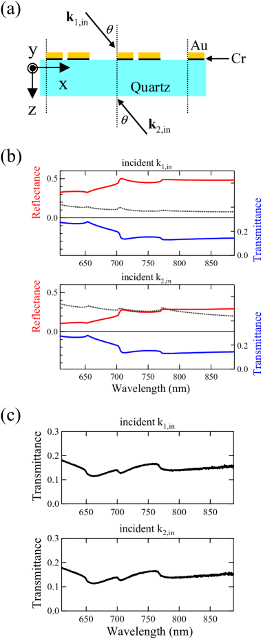
Figure 5: (a) Schematic drawing of metallic grating profile modeled from AFM images. The periodicity is 1200 nm. The dotted lines show the unit cells in which the ratio is Au:air:Au:air = 3:1:4:5. The thickness of Au, Cr, and the quartz substrate is 40 nm, 5 nm, and 1 mm, respectively. (b) Numerically calculated spectra for 10^∘ incidence of ${\bf k}_{1,{\rm in}}$ (upper panel) and ${\bf k}_{2,{\rm in}}$ (lower panel) of TM polarization. In both panels the reflectance (upper solid line) and absorption (dotted line) are plotted using the left axis, while the transmittance (lower solid line) uses the right axis. (c) Measured transmittance spectra, corresponding to the transmittance spectra in (b).