Temporal behavior of two-wave-mixing in photorefractive InP:Fe
versus temperature

Abstract

The temporal response of two-wave-mixing in photorefractive InP:Fe under a dc electric field at different temperatures has been studied. In particular, the temperature dependence of the characteristic time constant has been studied both theoretically and experimentally, showing a strongly decreasing time constant with increasing temperature.

I Introduction

The photorefractive effect leads to a variety of nonlinear optical phenomena in certain types of crystals. The basic mechanism of the effect is the excitation and redistribution of charge carriers inside a crystal as a result of non-uniform illumination. The redistributed charges give rise to a non-uniform internal electric field and thus to spatial variations in the refractive index of the crystal through the Pockels effect. Significant nonlinearity can be induced by relatively weak ($\mathrm{\SIUnitSymbolMicro}\mathrm{W}$) laser radiation. Phenomena such as self-focusing, energy coupling between two coherent laser beams, self-pumped phase conjugation, chaos, pattern formation and spatial soliton have attracted much attention in the past 20 years Yeh93 ; Haw99 .

Among photorefractive crystals, semiconductor materials have attractive properties for applications in optical telecommunications such as optical switching and routing. This is due to the fact that they are sensitive in the infrared region and their response time can be fast ($\mathrm{\SIUnitSymbolMicro}\mathrm{s}$)Sch02ol1229 .
Two-wave-mixing is an excellent tool to characterize the photorefractive effect in these materials Idr87oc317 ; Pic89ap3798 ; Mar99ap77 by determining the gain of amplification under the influence of the applied field, impurity densities, or grating period. Some semiconductors, like InP:Fe, exhibit an intensity dependant resonance at stabilized temperatures Pic89ap3798 ; Idr87oc317 .

In this paper, we analyze the temperature dependance of Two-Wave-Mixing (TWM) characteristic time constant, theoretically at first and eventually against experimental results. We propose a formal description of the temporal evolution of carrier densities in the medium, linking them to the TWM gain temporal evolution.

II Time dependant space-charge field in $InP:Fe$

The basic principles of the photorefractive effect in InP:Fe are well known Mar99ap77 . It involves three steps: photoexcitation of trapped carriers into excited states, migration of excited carriers preferentially towards non-illuminated regions and capture into empty deep centers. This leads to the formation of a local space-charge field $E_{sc}$ and thus to the modulation of the refractive index. The modulated refraction index is then able to interact with the beams that have created it. When the modulation stems from beam interference as in two wave mixing, an energy transfer between beams may occur.

The principle of two-wave-mixing is to propagate simultaneously in a photorefractive crystal two coherent beams, which have an angle $\theta$ between their directions of propagation. This phenomena is governed by the following system of coupled nonlinear differential equations:

$$\frac{dI_{s}}{dz} =\frac{\Gamma.I_{s}.I_{p}}{I_{0}}-\alpha.I_{s}$$ (1)

$$\frac{dI_{p}}{dz} =\frac{-\Gamma.I_{s}.I_{p}}{I_{0}}-\alpha.I_{p}$$ (2)

where $I_{p}$ is the pump intensity, $I_{s}$ is the signal intensity, and $I_{0}$ is the total intensity equal to the sum $I_{s}+I_{p}$, $\alpha$ is the absorption coefficient (assumed here to be the same for pump and signal). In a photorefractive crystal, $\Gamma$ takes the following form Pic89ap3798 :

$$\Gamma_{0} = (\frac{2.\pi.n^{3}.r_{eff}}{\lambda.\cos\theta}).Im\{E_{sc}\}$$ (3)

where $n$ is the refractive index, $r_{eff}$ is the effective electro-optic coefficient, $\lambda$ is the beam wavelength in vacuum and $Im\{E_{sc}\}$ is the imaginary part of the space-charge field $E_{sc}$(the $\frac{\pi}{2}$ shifted component of $E_{sc}$ with respect to the illumination grating). The expression of $E_{sc}$ will derived in the following lines. $\theta$ is the angle between the two beams.

In order to evaluate the photorefractive gain $\Gamma_{0}$ given by equation (3), the space-charge field $E_{sc}$ has to be calculated from the modified Kukhtarev model Kuk79fe949 , taking into account both electrons and holes as charge carriers. We chose a model with one deep center donor, two types of carriers (electrons and holes)str86ol312 , considering variations only in one transversal dimension (x) as described by the following set of equations:

$$\frac{dE}{dx} = \frac{e}{\epsilon}(N_{D}-N_{A}+p_{h}-n_{e}-n_{T})$$ (4a)

$$j_{n} = e\mu_{n}n_{e}E+\mu_{n}k_{b}T\frac{dn_{e}}{dx}$$ (4b)

$$j_{p} = e\mu_{p}p_{e}E-\mu_{p}k_{b}T\frac{dp_{h}}{dx}$$ (4c)

$$\frac{dn_{e}}{dt} = e_{n}n_{T}-c_{n}n_{e}p_{T}+\frac{1}{e}\frac{dj_{n}}{dx}$$ (4d)

$$\frac{dp_{h}}{dt} = e_{p}p_{T}-c_{p}p_{h}n_{T}-\frac{1}{e}\frac{dj_{p}}{dx}$$ (4e)

$$\frac{dn_{T}}{dt} = e_{p}p_{T}-e_{n}n_{T}-c_{p}p_{h}n_{T}+c_{n}n_{e}p_{T}$$ (4f)

$$N_{T} = n_{T}+p_{T}$$ (4g)

$$\int_{-d/2}^{d/2}Edx = V_{app}$$ (4h)

$$E =E_{app}+E_{sc}$$ (4i)

where $E$ is the electric field, $n_{e}$ and $p_{h}$ are the electron and hole densities in the respective conduction and valence bands, $n_{T}=Fe^{2+}$ is the density of ionized occupied traps, $p_{T}=Fe^{3+}$ is the density of neutral unoccupied traps, $J_{n}$ and $J_{p}$ are respectively the electron and hole currents. $N_{T}$, $N_{D}$ and $N_{A}$ are respectively the densities of iron atoms, the shallow donors and the shallow acceptors. The charge mobilities are given by $\mu_{n}$ for electrons and $\mu_{p}$ for holes, the electron and hole recombination rate are respectively $c_{n}$ and $c_{p}$ , $T$ is the temperature and $k_{b}$ is the Boltzmann constant. The dielectric permittivity is given by $\epsilon$ while $e$ is the charge of the electron. $V_{app}$ is the voltage applied externally to the crystal of width $d$. The electron and hole emission parameters are $e_{n}$ and $e_{p}$ depend on both thermal and optical emission as described by:

$$e_{n} =e^{th}_{n}+\sigma_{n}\frac{I(x)}{h\nu}$$ (5)

$$e_{p} =e^{th}_{p}+\sigma_{p}\frac{I(x)}{h\nu}$$ (6)

where the thermal contribution to the emission rate coefficient is $e^{th}$ and the optical cross section of the carriers is given by $\sigma$, $I(x)$ is the spatially dependent intensity of light due to the interferences between pump and signal beams and $h\nu$ is the photon energy.

For sufficiently small modulation depth $m$, intensity and all carriers densities may be expanded into Fourier series interrupted after the first term :

$$A(x)=A_{0}+A_{1}e^{iK_{g}x}$$ (7)

where $A(x)$ takes the role of $I$, $n_{e}$, $p_{h}$, $n_{T}$, $p_{T}$ and $K_{g}$ the spatial frequency of the interference pattern. So the light intensity can be written for the average intensity $I_{0}$ as:

$$I(x)=I_{0}(1+me^{iK_{g}x})$$ (8)

In the following, we have calculated the temporal evolution of carriers density and we will look forward to finding the temporal evolution of the space charge field under these hypothesis, i.e. considering only the zero’th and first order of the Fourier expansion.

The zero’th order corresponds to an uniform illumination ( $I(x)=I_{0}$). The space charge field is thus equal to zero and the local field is uniform and equals the applied field $E_{app}$. The electrons and holes densities at steady state are known to be equal to $\frac{e_{n}.n_{T_{0}}}{c_{n}.p_{T_{0}}}$ and $\frac{e_{p}.p_{T_{0}}}{c_{p}.n_{T_{0}}}$ respectively Pic89ap3798 , where $n_{T_{0}}$, $p_{T_{0}}$ are the density of occupied and unoccupied traps at steady state.

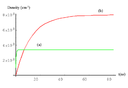
Figure 1: Temporal evolution of electron (a) and hole densities (b) under uniform illumination for $\lambda=1.06\leavevmode\nobreak\ \mathrm{\SIUnitSymbolMicro}\mathrm{m}$, $I_{0}=20\leavevmode\nobreak\ \mathrm{m}\mathrm{W}\mathrm{/}\mathrm{c}\mathrm{m}\mathrm{{}^{2}}$, T=297K. Materials parameters taken from ref Pic89ap3798 are: $c_{n}=4.1\times 10^{-8}\mathrm{c}\mathrm{m}^{3}\mathrm{/}\mathrm{s}$, $c_{p}=1.6\times 10^{-8}\mathrm{c}\mathrm{m}^{3}\mathrm{/}\mathrm{s}$, $e_{p}^{th}=10^{-4}\mathrm{s}^{-1}$, $e_{n}^{th}=16.32\mathrm{s}^{-1}$,  $n_{T_{0}}=5\times 10^{15}\mathrm{c}\mathrm{m}^{-3}$, $p_{T_{0}}=6\times 10^{16}\mathrm{c}\mathrm{m}^{-3}$, $n_{0}=1\times 10^{7}\mathrm{c}\mathrm{m}^{-3}$, $p_{0}=6\times 10^{6}\mathrm{c}\mathrm{m}^{-3}$, $\sigma_{n}=4\times 10^{-18}\mathrm{c}\mathrm{m}^{2}$, $\sigma_{p}=1\times 10^{-17}\mathrm{c}\mathrm{m}^{2}$ .

The electrons and holes densities in transient regime when an uniform illumination is established, are calculated by solving equations (4d) and (4e) , assuming that $I_{0}=0$ for $t<0$ and at time $t=0$, the carriers density values are equal to $n_{0}$ and $p_{0}$ at thermal equilibrium, without any optical excitations Haw99 . We obtained the following solution:

$$n_{e}(t) =\frac{e^{-c_{n}p_{T_{0}}t}(c_{n}p_{T_{0}}n_{0}+(-1+e^{c_{n}p_{T_{0}}t})n_{T_{0}}(e_{n}^{th}+\sigma_{n}\frac{I_{0}}{h\nu}))}{c_{n}p_{T_{0}}}$$ (9)

$$p_{h}(t) =\frac{e^{-c_{p}n_{T_{0}}t}(c_{p}n_{T_{0}}p_{0}+(-1+e^{c_{p}n_{T_{0}}t})p_{T_{0}}(e_{p}^{th}+\sigma_{p}\frac{I_{0}}{h\nu}))}{c_{p}n_{T_{0}}}$$ (10)

The temporal evolution of carrier densities under uniform illumination is illustrated in figure 1. Our model confirms the fact that the carrier densities evolution grows exponentially. The rise time of carriers generation is on the order of nanosecond time scale for a beam intensity of a few m W  per c m ^ 2 . Without presence of the beam, the electron density is greater than the hole density because electrons are mostly generated thermally while holes are generated optically Pic89ap3798 .

For a modulated intensity (first Fourier order), by using the set of equations (4), the space-charge field can be approximatively expressed at steady state as Pic89ap3798 :

$${\color[rgb]{0.98,0.00,0.00}E_{1}=\frac{i.m.I_{0}}{(I_{res}+I_{0})(\frac{1}{E_{q}}+\frac{E_{d}}{E_{0}^{2}+E_{d}^{2}})+i(I_{res}-I_{0})\frac{E_{0}}{E_{0}^{2}+E_{d}^{2}}}\approx m.E_{sc}}$$ (11)

where $E_{0}$, $E_{d}=K_{g}\frac{k_{b}.T}{e}$ and $E_{q}=\frac{e}{\epsilon.K_{g}}.\frac{n_{T_{0}}.p_{T_{0}}}{n_{T_{0}}+p_{T_{0}}}$ are the space charge field under uniform illumination, the diffusion field and charge-limiting field respectively. $I_{res}=\frac{e_{n}^{th}.n_{T_{0}}}{\sigma_{p}.p_{T_{0}}.h.\nu}$ is the resonance intensity defined as the intensity at which holes and electrons are generated at the same rate.

From equation (11), we observe that the space charge field is purely imaginary, when the illumination $I_{0}$ equals $I_{res}$. Above resonance, the hole density is higher than the electron one, mainly because the holes cross section is stronger than for electrons. The result is that charge transfer mainly occurs between iron level and the valence band. Below resonance, when electrons are dominant, the iron mainly interacts with the electrons and the conduction band.
In transient regime for a modulated intensity, the dynamics of the space charge field is calculated by considering an adiabatic approximations valqe1983 , a concentration of electrons and holes densities reaches instantaneously the equilibrium value which depends on the actual concentration of filled and empty traps, so we set: $\frac{dp_{h}}{dt}=\frac{dn_{e}}{dt}=0$. We assume that the electrons are excited thermally while the holes optically Pic89ap3798 . In the low modulation approximation, some algebraic manipulations of the set of equations (4) lead to:

$$E_{1}(t)=mE_{sc}[1-exp(-\frac{t}{\tau_{g}})]$$ (12)

where $\tau_{g}$ is a complex time constant, which can be rewritten by separating its real and imaginary parts.

$$\frac{1}{\tau_{g}} =\frac{1}{\tau}+iw$$ (13)

with

$$\tau =\frac{\tau_{n}\tau_{p}}{\tau_{n}+\tau_{p}}$$

and

$$w =w_{n}-w_{p}$$

The subscript indexes $n$ and $p$ are related to the electron and hole contributions respectively. $\tau_{n}$ and $w_{n}$ are given by:

$$\tau_{n} =\tau_{di,n}\frac{(1+\frac{Ed}{E_{Mn}})^{2}+(\frac{E_{0}}{E_{Mn}})^{2}}{(1+\frac{Ed}{E_{Mn}})(1+\frac{Ed}{Eq})+\frac{E_{0}^{2}}{(E_{Mn}.Eq)}}$$ (14)

$$w_{n} =\frac{1}{\tau_{di,n}}\frac{\frac{E_{0}}{E_{Mn}}-\frac{E_{0}}{Eq}}{(1+\frac{Ed}{E_{Mn}})^{2}+(\frac{E_{0}}{E_{Mn}})^{2}}$$ (15)

where $E_{Mn}=\frac{c_{n}.p_{T_{0}}}{\mu_{n}.k_{b}}$ is the mobility field, $\tau_{di,n}$ is the electron dielectric relaxation time depending on intensity and temperature which can be written as:

$$\tau_{di,n}=\frac{e_{n}^{th}.n_{T_{0}}.e.\mu_{n}}{c_{n}.p_{T_{0}}.\epsilon}$$ (16)

$e_{n}^{th}$ is the thermal parameter equal to:

$$e_{n}^{th}=3,25.10^{25}.\frac{m_{n}^{*}}{m}.T^{2}.\sigma_{n}^{\infty}.e^{\frac{-E_{na}}{k_{b}.T}}$$ (17)

where $\frac{m_{n}^{*}}{m}$ is the effective masse of electron, $E_{na}$ is the apparent activation energy of the electron trap, $\sigma_{n}^{\infty}$ is the electron capture cross section. The value of this parameters are determined experimentally bre81el55 .
To obtain $\tau_{p}$, $w_{p}$ and $\tau_{di,p}$, the index $p$ should be substituted for the index $n$ in the equations (14), (15) and (16).
From equations (12) to (17), it is possible to deduce, as was done previously Idr87oc317 ; Pic89ap3798 , that the time constant $\tau_{g}$ is real if electron emission is equal to the hole emission. That is, in the case of InP:Fe, electron thermal-emission is equal to the holes optical-emission. This allows to infer a link between the behavior of InP:Fe as a function of intensity and temperature.
It will be the aim of the following sections to confirm this link, both theoretically and experimentally

III Gain dynamics

The photorefractive gain $\Gamma$ is the main parameter that can be determined by two-wave-mixing. It quantifies an energy transfer from the pump beam to the signal beam and is proportional to the imaginary part of the space-charge field.

The gain value depends on different parameters like applied electric field, iron density $N_{T}$, pump intensity and temperature Ozksab1997 . Our work concentrate on the study of the gain dynamics versus temperature and we particularly analyze the dependance of the rise time on temperature.

The stationary value of the photorefractive gain at different temperatures is given by equation (3) where $E_{sc}$ is given by equation (11). This expression shows that a maximum gain is reached when $I_{0}=I_{res}$. This maximum corresponds to an intensity resonance Pic89ap3798 .

We studied theoretically the temporal gain behavior using the standard definition given by equation (18) deduced from equation (12) by developing $E_{sc}$ and $\tau_{g}$.

$$\Gamma=\Gamma_{0}[1+\exp(\frac{-t}{\tau})\times\frac{\sin(wt-\psi)}{\sin\psi}]$$ (18)

where
$\psi$: argument of stationary space-charge field ($E_{sc}=|E_{sc}|\exp{i\psi}$)
$\tau$: amplification’s characteristic rise time.

Our theoretical simulations produce the curves represented on figure 2, illustrating the evolution of photorefractive gain as function of time for three different pump beam intensities: at resonance, below and above resonance for

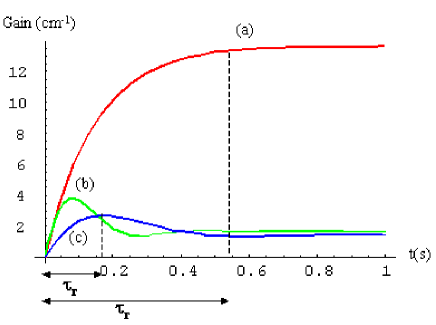
Figure 2: Temporal evolution of local gain at different intensities at $T=297K$ ($e_{n}^{th}=16.31\mathrm{s}^{-1}$ calculated from equation 17),  $\Lambda=5\leavevmode\nobreak\ \mathrm{\SIUnitSymbolMicro}\mathrm{m}$,  $E_{0}=10\leavevmode\nobreak\ \mathrm{k}\mathrm{V}\mathrm{/}\mathrm{c}\mathrm{m}$, crystal thickness $L=12mm$ : (a) $I_{0}=25.5\leavevmode\nobreak\ \mathrm{m}\mathrm{W}\mathrm{/}\mathrm{c}\mathrm{m}\mathrm{{}^{2}}\sim Ires$, (b) $I_{0}=15\leavevmode\nobreak\ \mathrm{m}\mathrm{W}\mathrm{/}\mathrm{c}\mathrm{m}\mathrm{{}^{2}}$,  (c)$I_{0}=50\leavevmode\nobreak\ \mathrm{m}\mathrm{W}\mathrm{/}\mathrm{c}\mathrm{m}\mathrm{{}^{2}}$.  $\tau_{r}$: characteristic time constant of amplification.

the same parameters as in figure 1. We see that the gain amplitude differs from each intensity to another, it takes the maximum value around resonance.

As a next step, we studied theoretically the TWM gain time response as a function of temperature. For an easier comparison with experimental results, in the following, the response time is $\tau_{r}$ will be considered as the time interval necessary for the gain to reach $90\%$ of the first maximum of each curves as shown in figure 2. The response time $\tau_{r}$ versus temperature are given in figure 3 for three distinct intensities, along with a fourth fitted curve showing the time constant at resonance intensities. We observe that the response time quickly decays as temperature increases. At resonance, $\tau_{r}$ is larger because the space charge field is high and it consequently necessitates more charge to accumulate.

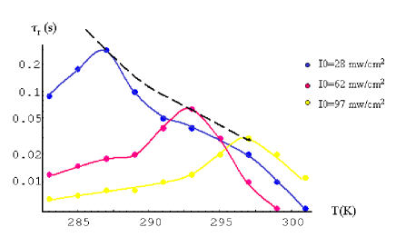
Figure 3: Characteristic time of amplification versus temperature at three different intensities. The time constant at the resonance intensity is given for each temperature by the dotted line.

IV Average gain

The theoretical curve shown in figure 2, illustrates the temporal evolution of the local gain. For the InP:Fe sample, the absorption coefficient at $\lambda=1.06\mu m$ being approximately equal to $1cm^{-1}$. Owing to this absorption, the mean intensity decrease along the $z$ axis propagation. The exponential gain would result from an integration over the optical thickness, as described in equation 19.

$$\Gamma=\frac{1}{L}\int^{L}_{0}\Gamma(z).dz$$ (19)

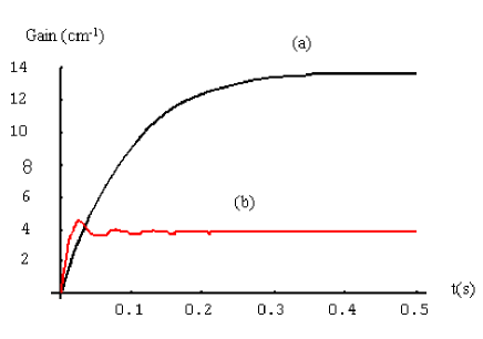
Figure 4: Local (a) and average gain (b) versus time, $I_{0}=25.5\leavevmode\nobreak\ \mathrm{m}\mathrm{W}\mathrm{/}\mathrm{c}\mathrm{m}\mathrm{{}^{2}}$,  $e_{n}^{th}=16.31\mathrm{s}^{-1}$, $\Lambda=5\leavevmode\nobreak\ \mathrm{\SIUnitSymbolMicro}\mathrm{m}$, $E_{0}=10\leavevmode\nobreak\ \mathrm{k}\mathrm{V}\mathrm{/}\mathrm{c}\mathrm{m}$.

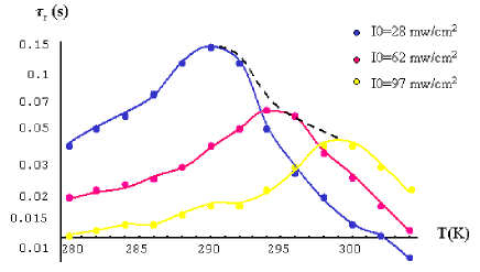
Figure 5: Average gain characteristic time versus temperature at three different intensities. The time constant at the resonance intensity is given for each temperature by the dotted line.

The figure 4 shows temporal evolution of local and average gain for $L=12mm$ crystal thickness for the same intensity; the average gain is lower because the intensity absorption is taken into account.

Because of the absorption the resonance intensity for average gain is higher than the local one for the same temperature. As for the local gain, we calculated numerically the characteristic time, in the same way. The results are shown in figure 5. We compare the results in figure 3, we observe the following differences: the resonance peaks are slightly widened because is reached within the example for various input intensities and the peaks are shifted towards high intensities again because of absorption. These conclusions can arise from figures 3 and 5 although they show the rise time as a function of temperature. Indeed, our calculations show that the photorefractive gain and rise time are linked, so that the rise time is the slowest for the highest gain (i.e. at resonance); since more charges need to be accumulated.

V Experimental validation

We perform standard two-wave mixing experiments in co-directional configuration as shown in figure 6. Pump and signal beam intensities ratio is set to $\beta=50$ and the angle between pump and signal is $2\theta=12^{0}$ corresponding for an space grating $\Lambda=5\mu m$. The experiments are performed with a CW $1.06\mathrm{\SIUnitSymbolMicro}\mathrm{m}$ YAG laser.

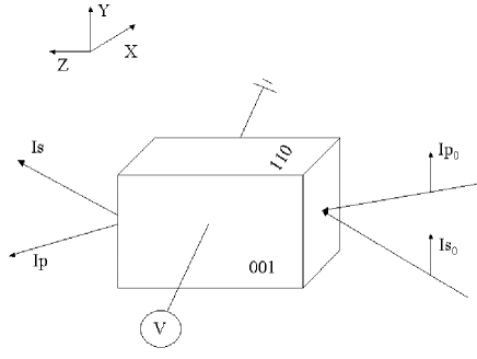
Figure 6: Two-wave-mixing configuration.

An electric field ($10\mathrm{k}\mathrm{V}\mathrm{/}\mathrm{c}\mathrm{m}$) is applied between the $<001>$ faces of InP:Fe crystal ($5\times 5\times 12mm^{3}$). The light beam is linearly polarized along the $<\overline{1}10>$ direction and propagates along the $<110>$ direction ($12mm$). The absorption constant as measured by spectrometer is close to $1cm^{-1}$ at $1.06\mu m$. Crystal temperature is stabilized by a Peltier cooler.

Transient behavior is analyzed by measuring $\tau_{r}$ as was done in figures 3 and 5. Figure 7 shows the results obtained for three different intensities from one side to the other of the resonance (the oscillations seen on figure 7 are attributed to the experimental noise and the curves are assumed to correspond to the first order responses). Experimental results concerning the TWM time constant are given on figure 8. For high temperature, $\tau_{r}$ decreases for all intensities.

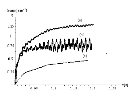
Figure 7: Gain dynamics at 288K at different intensities: (a)$62\leavevmode\nobreak\ \mathrm{m}\mathrm{W}\mathrm{/}\mathrm{c}\mathrm{m}\mathrm{{}^{2}}$,(b)$97\leavevmode\nobreak\ \mathrm{m}\mathrm{W}\mathrm{/}\mathrm{c}\mathrm{m}\mathrm{{}^{2}}$ (c)$28\leavevmode\nobreak\ \mathrm{m}\mathrm{W}\mathrm{/}\mathrm{c}\mathrm{m}\mathrm{{}^{2}}$.

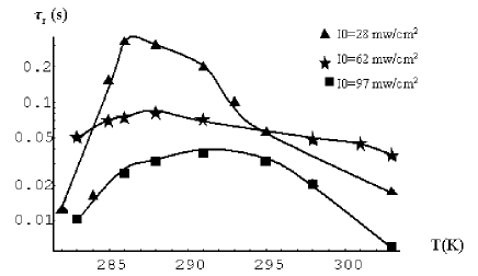
Figure 8: The $\tau_{r}$ versus temperature at different intensities.

Note that, for both theory and experiments, $\tau_{r}$ value decreases from $300$ to $50\leavevmode\nobreak\ \mathrm{m}\mathrm{s}$ for an increase temperature of $10^{0}C$–showing a good quantitative result. The discrepancy observed between figure 8 and 3 is partially corrected by taking into account the gain integration along the beam path inside the crystal, as shown in figure 5, showing a widening of the curves. We attribute the difference observed in terms of gain maximum value to lack of precision in the knowledge of the crystal’s physical constants such as photo-excitation, cross section and dopant concentration.

VI Conclusion

We have studied the dynamics of TWM in InP:Fe as a function of intensity and temperature. A theoretical analysis shows that the gain coefficient oscillates when an intensity lower or higher than the resonance intensity is used. At resonance the gain grows exponentially.

The experimental study shows that the crystal absorption prevents the oscillating behavior. We have shown that the gain rise time is strongly temperature dependent. Experimentally the gain rise time is $10$ times shorter at $295K$ than at $285K$ for low intensities.

According to experimental and applications needs, the temperature as well as the intensity can be used to tune the photorefractive response time.

References

- (1) P. Yeh. Introduction to photorefractive nonlinear optics. Wiley series in pure and applied optics, New York, 1993.
- (2) S.A. Hawkins. Photorefractive optical wires in the semiconductor Indium Phosphide. PhD thesis, Rose-Hulman Institute of technology , University of Arkansas.
- (3) T. Schwartz, Y. Ganor, T. Carmon, R. Uzdin, S. Shwartz, M. Segev, and U. El-Hanany. Photorefractive solitons and light-induced resonance control in semiconductor CdZnTe. Opt.Lett., 27(14):1229, 2002.
- (4) A. A-Idrissi, C. Ozkul, N. Wolffer, P. Gravey, and G. Picoli. Resonant behaviour of the temporal response of the two-wave mixing in photorefractive InP:Fe crystals under dc fields. Opt. Comm., 86:317–323, 1991.
- (5) G. Picoli, P. Gravey, C. Ozkul, and V. Vieux. Theory of two-wave mixing gain enhancement in photorefractive InP:Fe : A new mecanism of resonance. Appl.Phys., 66:3798, 1989.
- (6) G. Martel, A. Hideur, C. Ozkul, M. Hage-Ali, and J.M. Koebbel. Stationary and transient analysis of photoconductivity and photorefractivity in CdZnTe. Appl.Phys.B., 70:77–84, 1999.
- (7) N.V. Kukhtarev, V.B. Markov, S.G. Odulov, M.S. Soskin, and V.L. Vinetskii. Holographic storage in electrooptic crystals, beam coupling light amplification. Ferroelectrics., 22:961–964, 1979.
- (8) F.P. Strohkendl, J.M.C. Jonathan, and R. W. Hellwath. Hole-electron competition in photorefractive gratings. Opt. Lett., 11(5):312–314, 1986.
- (9) G. C. Valley. Short-pulse grating formation in photorefractive materials. IEEE J. Quantum Electron, 19:1637–1645, 1983.
- (10) G.Bremond, A.Nouailhat, G.Guillot, and B.Cockayne. Deep level spectropscopy in . Electron. Lett., 17:55–56, 1981.
- (11) Cafer Ozkul, Sophie Jamet, and Valerie Dupray. Dependence on temperature of two-wave mixing in InP:Fe at three different wavelengths: an extented two-defect model. Soc. Am. B, 14(11):2895–2903, 1997.