Collisional broadening of alkali doublets by helium perturbers

Abstract

We report results for the Lorentzian profiles of the Li I, Na I and K I doublets and the Na I subordinate doublet broadened by helium perturbers for temperatures up to 3000 K. They have been obtained from a fully quantum-mechanical close-coupling description of the colliding atoms, the Baranger theory of line shapes and new ab initio potentials for the alkali-helium interaction. For all lines except the 769.9 nm K I line, the temperature dependence of the widths over the range $70\leq T\leq 3000$ K is accurately represented by the power law form $w=aT^{b}$ with $0.37<b<0.43$. The 769.9 nm K I line has this form for $500\leq T\leq 3000$ K with $b$ having the higher value of 0.49. Although the shifts have a more complex temperature dependence, they all have the general feature of increasing with temperature above $T\sim 500$ K apart from the 769.9 K I line whose shift decreases with temperature.

1 Introduction

Accurate pressure broadened profiles of alkali resonance doublets perturbed by H₂ and He are of crucial importance for the modelling of atmospheres of late M, L and T type brown dwarfs and for generating their synthetic spectra in the region 0.6 - 1.1 $\mu$m. The dominant lines are the Na I 589.0/589.6 nm and K I 766.5/769.9 nm doublets [1, 2] which occur in the middle of a spectral region where background absorption is particularly small so that both the line centres and wings stand out. There can also be significant contributions from less abundant alkalis such as Li, Rb and Cs, and from subordinate doublets such as Na I 818.3/819.5 nm.

The profiles of the strongly broadened alkali doublets have been the subject of several recent studies using models primarily designed to describe the non-Lorentzian far wings of the profiles. Burrows and Volobuyev [3] used a quasistatic unified Franck-Condon semiclassical model to study the Na I and K I doublets whereas a unified line shape semiclassical model has been used by Allard et al[4] for the Na I and K I doublets and, more recently, for the Rb I and Cs I doublets [5]. Alternatively, quantum mechanical single-channel models based upon bound-free and free-free transitions in the transient molecules formed during collision have been used to calculate the emission and absorption spectra for the wings of the Li I [6, 7], Na I [6, 8] and K I [8] resonance lines in the presence of He perturbers. Despite these studies, highly accurate calculations of the central Lorentzian cores are still needed in order to estimate the effects of dust in brown dwarf atmospheres.

We report results for the widths and shifts of the Lorentzian profiles over the temperature range $70\leq T\leq 3000$ K of the Li I, Na I and K I doublets and the Na I subordinate doublet broadened by helium perturbers. The calculations extend our previous study [9] of pressure broadening of the Na I doublets by He at laboratory temperatures up to 500 K and are based on a fully quantum-mechanical close-coupling description of the colliding atoms and the Baranger [10] theory of line shapes. As input for our calculations we have computed new ab initio potentials for the alkali-helium interaction. Preliminary results for the widths of two Na I lines for temperatures up to 2000 K have been given in [11] and for the widths of the Na I and K I doublets in [12].

2 Interatomic potentials

The adiabatic molecular potentials ${}^{2S+1}V_{\Lambda}(R)$ for the X^∗–He system (where X = Li, Na or K) have been obtained by using a three-body model in which the alkali X^∗ is treated as a X⁺ ion plus an active electron and the perturbing He atom is represented by a polarizable atomic core. Model potentials are used to represent the electron-atom and electron-atomic ion interactions and the basic methods adopted for obtaining these model potentials are discussed by [13]. These potentials reproduce not only the correct energies of the bound states of X^∗ but also generate wavefunctions for both the bound and scattering states of X$+e^{-}$ and He$+e^{-}$ that contain the correct number of nodes. The model potentials also support unphysical bound states corresponding to the presence of closed shells in the X⁺ ion and in He. This effect is taken into account in the calculation of the molecular potential by including the unphysical states in the atomic basis used in the diagonalization of the Hamiltonian for the three-body model.

The most important recent change from the earlier approach is that the core-core interaction is itself calculated directly using a three-body model composed of X⁺ and He⁺ cores plus one electron. A more detailed discussion of this development is given for the Li-He case by [14]. Further numerical refinements have been incorporated into the computer program since then and new calculations carried out for the three alkali-helium systems considered in our study.

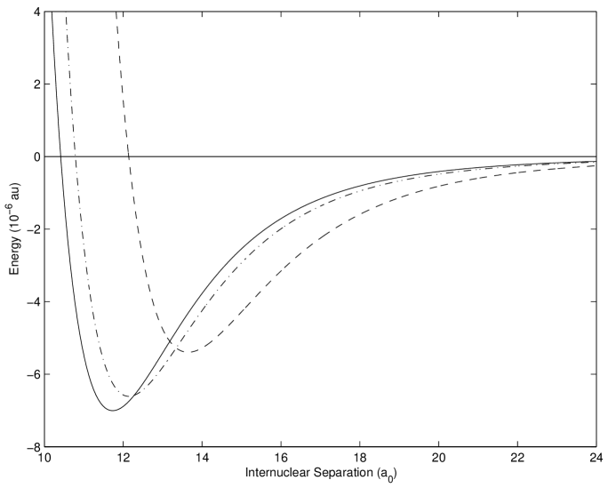
Figure 1: Adiabatic ns ${}^{2}V_{\Sigma}$ molecular potentials: Li-He (——), Na-He (— $\cdot$ —) and K-He (– – –).

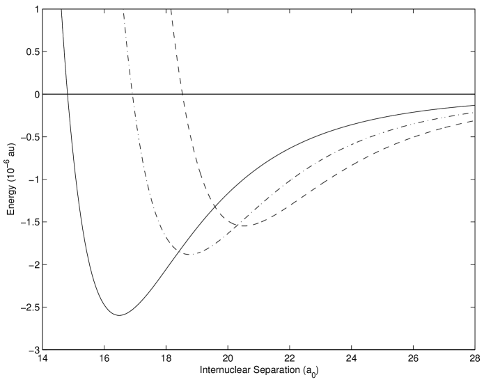
Figure 2: Adiabatic np ${}^{2}V_{\Sigma}$ molecular potentials: Li-He (——), Na-He (— $\cdot$ —) and K-He (– – –).

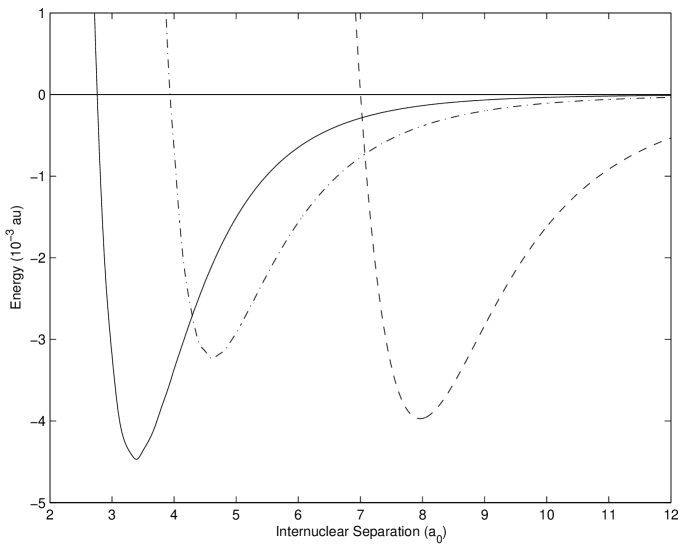
Figure 3: Adiabatic np ${}^{2}V_{\Pi}$ molecular potential: Li-He (——), Na-He (— $\cdot$ —) and K-He (– – –). Note that the Na-He and K-He potentials have been scaled up by factors of 5 and 20 respectively.

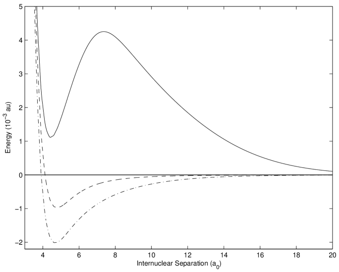
Figure 4: Adiabatic potential curves for Na-He: 3d ${}^{2}V_{\Sigma}$ (——), 3d ${}^{2}V_{\Pi}$ (— $\cdot$ —) and 3d ${}^{2}V_{\Delta}$ (– – –).

The ns ${}^{2}V_{\Sigma}$, np ${}^{2}V_{\Sigma}$ and np ${}^{2}V_{\Pi}$ molecular potentials for Li-He $(n=2)$, Na-He $(n=3)$ and K-He $(n=4)$ are shown in figures 1, 2 and 3 respectively. The Na-He 3d ${}^{2}V_{\Sigma,\Pi,\Delta}$ potentials are shown in figure 4. The minima in the potentials used and their positions are given in tables 1, 2 and 3 and compared with other data where they are available. New ab initio potentials for K-He have recently been obtained [27] but no details are given. The overall agreement with other work is very satisfactory and the three-body model can be expected to give good results at medium and large interatomic separations. However the positions of the minima in the np ${}^{2}V_{\Pi}$ potentials occur at short range and are largely determined by the behaviour of the core-core interaction. For the Li-He and Na-He cases the agreement with theory and experiment for the np ${}^{2}V_{\Pi}$ states is generally good, but the result for the K-He 4p ${}^{2}V_{\Pi}$ state requires some comment. Because the 3p virtual state supported by the K${}^{+}+e^{-}$ model potential has a higher energy than that of He(1s²), the core-core potential, K⁺-He, is unreliable at small separations. Methods for resolving this difficulty are still being investigated, but since the behaviour of line widths and shifts depends largely on the difference between upper and lower state potentials they are not particularly sensitive to this problem.

3 Spectral line profile

The width and shift of each spectral line have been calculated using the quantum-mechanical impact theory of Baranger [10] for non-overlapping spectral lines in which the profile of each isolated line is a Lorentzian. The orbital, spin and total electronic angular momentum operators for the alkali atom are $\mathbf{L}$, $\mathbf{S}$ and $\mathbf{j}=\mathbf{L}+\mathbf{S}$ respectively and radiation is emitted by the alkali atom as it undergoes a transition between initial and final states $|n_{i}L_{i}S_{i}j_{i}\rangle$ and $|n_{f}L_{f}S_{f}j_{f}\rangle$, where $n$ denotes the principal quantum number. The half half-width $w$ and shift $d$ at temperature $T$ of the Lorentzian profile is given by [31]

$$w+\rmi d=N\;\int_{0}^{\infty}\;f(E)\;S(E)\;\rmd E$$ (1)

where $f(E)$ is the normalized Maxwellian perturber energy distribution

$$f(E)=2\pi(\pi k_{{\rm B}}T)^{-3/2}\>\sqrt{E}\;\exp[-E/(k_{{\rm B}}T)],$$ (2)

$N$ is the perturber number density and

$$S(E)=\frac{\hbar^{2}\pi}{M^{2}}\sqrt{\frac{M}{2E}}\;\sum_{l,l^{\prime}}\;\sum_{J_{i},J_{f}}(2J_{i}+1)(2J_{f}+1)(-1)^{l+l^{\prime}}\left\{{J_{f}\;J_{i}\;1\atop j_{i}\;j_{f}\;l}\right\}\left\{{J_{f}\;J_{i}\;1\atop j_{i}\;j_{f}\;l^{\prime}}\right\}$$

$$\times[\delta_{l,l^{\prime}}-\langle j_{i}\;l^{\prime}\;J_{i}|S|j_{i}\;l\;J_{i}\rangle\langle j_{f}\;l^{\prime}\;J_{f}|S|j_{f}\;l\;J_{f}\rangle^{*}]$$ (3)

describes the effects of collisions on the two states forming the spectral line. Here $M$ is the reduced mass of the emitter-perturber system, $l$ and $l^{\prime}$ are quantum numbers corresponding to the relative emitter-perturber angular momentum $\mathbf{L}_{R}$ before and after the collision and $\mathbf{J}=\mathbf{L}_{R}+\mathbf{j}$ is the total angular momentum of the emitter-perturber system. The scattering matrix element in the coupled $|j\;l\;J\rangle$ representation is $\langle j^{\prime}\;l^{\prime}\;J|S|j\;l\;J\rangle$ where we have suppressed the quantum numbers $(n,L,S)$ for convenience and $\left\{{a\;b\;c\atop f\;g\;h}\right\}$ is the $6-j$ symbol [32].

The scattering matrix elements in (3) are determined from the asymptotic behaviour of the radial functions $G^{J}_{jl}(R)$ for each scattering channel $(j,l,J)$. These functions satisfy the coupled equations [31]

$$[\frac{\partial^{2}}{\partial R^{2}}-\frac{l(l+1)}{R^{2}}+k_{j}^{2}]G^{J}_{jl,j^{\prime\prime}l^{\prime\prime}}(R)=\frac{2M}{\hbar^{2}}\sum_{j^{\prime},l^{\prime}}\;V^{J}_{jl,j^{\prime}l^{\prime}}(R)\;G^{J}_{j^{\prime}l^{\prime},j^{\prime\prime}l^{\prime\prime}}(R),$$ (4)

where $(j^{\prime\prime},l^{\prime\prime})$ labels the linearly independent solutions of (4) and the Born-Oppenheimer coupling terms have been neglected. The parameter

$$k_{j}^{2}=2M[E-(E^{(L,S)}+\varepsilon_{j}(\infty))]/\hbar^{2}$$ (5)

is positive for open scattering channels and negative for closed channels. Here $E$ is the total energy of the emitter-perturber system, $E^{(L,S)}$ is the energy of the state of the separated atoms to which the molecular state dissociates adiabatically and the fine structure parameter $\varepsilon_{j}(R)$ has been assumed to have its asymptotic value $\varepsilon_{j}(\infty)$. The interaction potential matrix elements $V^{J}_{jl,j^{\prime}l^{\prime}}(R)$ are, for the ns ${}^{2}\mathrm{S}_{j}$ level

$$V_{jl,j^{\prime}l^{\prime}}(R)=\delta_{j,j^{\prime}}\delta_{l,l^{\prime}}\;^{2}V_{\Sigma}(R),$$ (6)

for the np ${}^{2}\mathrm{P}_{j}$ levels,

$$V_{jl,j^{\prime}l^{\prime}}(R)=\delta_{j,j^{\prime}}\delta_{l,l^{\prime}}\;^{2}V_{\Pi}(R)+C^{(1)}_{jl,j^{\prime}l^{\prime}}[^{2}V_{\Sigma}(R)-\;^{2}V_{\Pi}(R)]$$ (7)

and, for the nd ${}^{2}\mathrm{D}_{j}$ levels

$$V_{jl,j^{\prime}l^{\prime}}(R)=\delta_{j,j^{\prime}}\delta_{l,l^{\prime}}\;^{2}V_{\Delta}(R)+(-1)^{j^{\prime}-j}[1+(-1)^{l^{\prime}+l}]B_{jl,j^{\prime}l^{\prime}}[^{2}V_{\Pi}(R)-\;^{2}V_{\Delta}(R)]$$

$$+C^{(2)}_{jl,j^{\prime}l^{\prime}}[^{2}V_{\Sigma}(R)-\;^{2}V_{\Delta}(R)]$$ (8)

where the coefficients

$$C^{(n)}_{jl,j^{\prime}l^{\prime}}=\sum_{\Omega}\;(-1)^{j^{\prime}-j}C(J\;j\;l;-\Omega\;\Omega\;0)C(J\;j^{\prime}\;l^{\prime};-\Omega\;\Omega\;0)$$

$$\times C(n\;{\textstyle\frac{1}{2}}\;j;0\;\Omega\;\Omega)C(n\;{\textstyle\frac{1}{2}}\;j^{\prime};0\;\Omega\;\Omega)$$ (9)

and

$$B_{jl,j^{\prime}l^{\prime}}=\sum_{\Omega}\;C(J\;j\;l;-\Omega\;\Omega\;0)C(J\;j^{\prime}\;l^{\prime};-\Omega\;\Omega\;0)$$

$$\times C(2\;{\textstyle\frac{1}{2}}\;j;1\;\Omega-1\;\Omega)C(2\;{\textstyle\frac{1}{2}}\;j^{\prime};1\;\Omega-1\;\Omega)$$ (10)

are symmetric under $(j,l)\leftrightarrow(j^{\prime},l^{\prime})$. Here $C(j_{1}j_{2}j_{3};\Omega_{1}\Omega_{2}\Omega_{3})$ is the Clebsch-Gordan coefficient, $\Omega$ denotes the projection of an angular momentum onto the internuclear axis $\bi{R}$ and ${}^{2S+1}V_{\Lambda}(R)$, where $\Lambda\equiv|\Omega_{L}|$, are the adiabatic molecular potentials.

The equations (4) decouple into two sets of opposite parity $(-1)^{J\pm 1/2}$. Thus the ns ${}^{2}\mathrm{S}_{j}$, np ${}^{2}\mathrm{P}_{j}$ and nd ${}^{2}\mathrm{D}_{j}$ states give rise to one, three and five coupled differential equations respectively for each parity. These equations were solved using a modified version [31] of the R-Matrix method of Baluja et al [33] and the solutions fitted to free-field boundary conditions to extract the scattering matrix elements.

4 Results and discussion

Calculations have been completed for the Li I doublet 2p ${}^{2}\mathrm{P}_{3/2,1/2}\rightarrow$ 2s ${}^{2}\mathrm{S}_{1/2}$, the Na I doublet 3p ${}^{2}\mathrm{P}_{3/2,1/2}\rightarrow$ 3s ${}^{2}\mathrm{S}_{1/2}$, the K I doublet 4p ${}^{2}\mathrm{P}_{3/2,1/2}\rightarrow$ 4s ${}^{2}\mathrm{S}_{1/2}$ and the Na I subordinate ”doublet” 3d ${}^{2}\mathrm{D}_{3/2}\rightarrow$ 3p ${}^{2}\mathrm{P}_{1/2}$ and 3d ${}^{2}\mathrm{D}_{5/2,3/2}\rightarrow$ 3p ${}^{2}\mathrm{P}_{3/2}$. The main computational issues associated with extending our previous calculations up to the higher temperatures (3000 K) of astrophysical interest are convergence of the sum over partial waves in (3) and of the integration (1) over perturber energies. The present calculations required about 500 partial waves for most of the energy nodes but up to 1000 partial waves were needed at the highest energy nodes which corresponded to temperatures extending to 5000 K.

The $R$-matrix propagation was commenced using the arbitrary choice $R=I$ at a distance $R_{\mathrm{min}}$ well within the classical turning point so that the solutions were independent of $R_{\mathrm{min}}$. Typically $R_{\mathrm{min}}$ ranged from $2a_{0}$ for small $l$ to $25a_{0}$ for large $l$. The distance $R_{\mathrm{max}}$ at which the solutions were matched to the free-field solutions was typically $300a_{0}-400a_{0}$. This yielded $S$-matrix elements accurate to at least six significant figures and, after summing over partial waves, resulted in six figure accuracy for $\Re S(E)$ and four for $\Im S(E)$. As the major part of the $R$-matrix method is energy independent, equations (4) are solved at each value of $l$ for the entire set of energy nodes. The large number of partial waves needed might suggest that a semiclassical treatment would be more appropriate. However the present quantal calculations did not require an inordinate amount of computer time (typically a few hours) and are free of the uncertainties endemic in semiclassical calculations of determining the appropriate lower cutoff on impact parameters in order to exclude perturber paths entering the classically forbidden regions of the interatomic interaction [31].

The temperature dependence of the computed half half-widths and shifts are shown in figures 5 and 6 respectively. The widths and shifts of all lines were calculated at 10 K intervals and in all cases were found to be smooth functions of temperature. The widths are accurately represented to three significant figures by the power law form

$$w(T)=aT^{b}$$ (11)

where the fit parameters $a$ and $b$ are given in table 4. Also shown are the values of $b$ obtained by [35] using a semiclassical model which does not resolve the members of each doublet. Our results agree closely with this early calculation except for the anomalous 4p ${}^{2}\mathrm{P}_{1/2}$ – 4s ${}^{2}\mathrm{S}_{1/2}$ potassium transition where our value is significantly higher. For all lines the temperature dependence is stronger than the $T^{0.3}$ behaviour obtained from a classical treatment using a pure van der Waals $V(R)=-C_{6}/R^{6}$ interaction.

Although the shifts have a more complex temperature dependence, they all have the general feature of increasing with temperature above $T\sim 500$ K apart from the 4p ${}^{2}\mathrm{P}_{1/2}$ – 4s ${}^{2}\mathrm{S}_{1/2}$ potassium transition which is again anomalous as its shift decreases with temperature.

The effects of fine structure on the calculated widths and shifts arises from the $6-j$ symbols in (3) and the $j$-dependence of the $S$-matrix due to the potential matrix elements $V_{jl,j^{\prime}l^{\prime}}(R)$ and the fine-structure splittings $\varepsilon_{j}(\infty)$ appearing in (4). However, as the zero energy for the calculation of any level ${}^{2S+1}\mathrm{L}_{j}$ is set at the energy $E_{0}=E^{(L,S)}+\varepsilon_{j}(\infty)$ of that level and the splittings are negligible for all but the lowest energy nodes, the role of the actual splittings is relatively unimportant. This is evident in the results for the Na lines 3d ${}^{2}\mathrm{D}_{5/2,3/2}\rightarrow$ 3p ${}^{2}\mathrm{P}_{3/2}$ where the widths and shifts are significantly different even though $\varepsilon_{3/2}(\infty)=\varepsilon_{5/2}(\infty)$.

The behaviour of the anomalous potassium transition warrants some comment. The calculation for the potassium 4p ${}^{2}\mathrm{P}_{1/2}$ level is different from that of all other levels considered in the present study in that there are closed channels at the lowest energy nodes and the wells of the molecular potentials are very shallow (depths $E_{d}<10^{-4}$ au), smaller than the fine structure splitting $\varepsilon=2.68\times 10^{-4}$ au of the level. Consequently the channels only become open at energies above $\varepsilon$ and therefore at energies above $E_{d}$.

We compare our calculated widths and shifts with measurement in table 5 and table 6 respectively. We have not included all the experimental width data for Na as the present calculations for the Na doublets closely reproduce our earlier results [9] for $T\leq 500$ K and a detailed comparison with the numerous existing theoretical and experimental studies was reported in that paper. In general the widths are in good agreement for all alkalis although only one measurement is for $T>700$ K. The situation regarding the shifts is less clear. The predicted shift for the 3d ${}^{2}\mathrm{D}_{3/2}$ – 3p ${}^{2}\mathrm{P}_{1/2}$ Na I line agrees very closely with the measurement of [40] and the results for the K I doublet have the same sign and relative magnitude as the measurements. However the predicted shifts for the Li I and Na I doublets have the opposite sign to that of the measured shifts. The shifts are quite sensitive to the precise details of the potentials as they are produced by a balance between the effects of the long-range attractive potential and the short-range repulsive potential. In particular, for a given energy they are sensitive to where the repulsive wall is located. Consequently the disagreement with experiment for the Li I and Na I doublets suggests that the repulsive region of the Li potential may need to be slightly suppressed and that of the Na potential enhanced.

References

=0.8

=0.8

=0.8

=0.8

=0.8

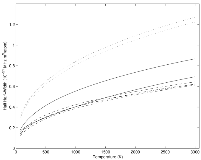
Figure 5: Temperature dependence of half half-widths (in units of $10^{-21}$ MHz m³/atom) of alkali lines perturbed by He. The doublets np ${}^{2}\mathrm{P}_{j}$ – ns ${}^{2}\mathrm{S}_{1/2}$ shown are Li (— $\cdot$ —), Na (– – –) and K (——) where the upper (lower) curve corresponds to $j=3/2(j=1/2)$. The Na lines 3d ${}^{2}\mathrm{D}_{j_{i}}$ – 3p ${}^{2}\mathrm{P}_{j_{f}}$ are shown (${\mathinner{\cdotp\cdotp\cdotp\cdotp\cdotp\cdotp}}$) with the upper curve corresponding to $(j_{i},j_{f})=(3/2,3/2)$ and $(3/2,1/2)$ unresolved and the lower curve to $(5/2,3/2)$. Note that, on the scale shown, the members of the Li doublet cannot be resolved.

=0.8

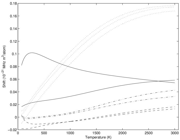
Figure 6: Temperature dependence of shifts (in units of $10^{-21}$ MHz m³/atom) of alkali lines perturbed by He. The doublets np ${}^{2}\mathrm{P}_{j}$ – ns ${}^{2}\mathrm{S}_{1/2}$ shown are Li (— $\cdot$ —), Na (– – –) and K (——) where the upper (lower) curve at the lower temperatures corresponds to $j=1/2(j=3/2)$. The Na lines 3d ${}^{2}\mathrm{D}_{j_{i}}$ – 3p ${}^{2}\mathrm{P}_{j_{f}}$ lines are shown (${\mathinner{\cdotp\cdotp\cdotp\cdotp\cdotp\cdotp}}$) with $(j_{i},j_{f})=(5/2,3/2)$ (upper curve), $(3/2,3/2)$ (middle curve) and $(3/2,1/2)$ (lower curve).

Tables and table captions

Table 1: Positions $R_{d}\,(a_{0})$ and minimum energies $V_{d}$ (au) of the Li-He adiabatic molecular potentials. Also given are the $C_{6}$ (au) coefficients for the asymptotic forms of the potentials.

2s ${}^{2}V_{\Sigma}$		2p ${}^{2}V_{\Sigma}$		2p ${}^{2}V_{\Pi}$
$R_{d}$	$V_{d}$	$R_{d}$	$V_{d}$	$R_{d}$	$V_{d}$
11.73	$-7.005\times 10^{-6}{\,}^{\rm a}$	16.48	$-2.596\times 10^{-6}{\,}^{\rm a}$	3.39	$-4.470\times 10^{-3}{\,}^{\rm a}$
11.553	$-6.787\times 10^{-6}{\,}^{\rm b}$	17.027	$-1.511\times 10^{-6}{\,}^{\rm c}$	3.395	$-4.55\times 10^{-3}{\,}^{\rm d}$
11.56	$-6.79\times 10^{-6}{\,}^{\rm e}$	18.0	$-1.4\times 10^{-6}{\,}^{\rm f}$	3.44	$-5.65\times 10^{-3}{\,}^{\rm g}$
12.2	$-9.1\times 10^{-6}{\,}^{\rm k}$	17.0	$-3.1\times 10^{-6}{\,}^{\rm h}$	3.44	$-4.670\times 10^{-3}{\,}^{\rm h}$
12.0	$-4.6\times 10^{-6}{\,}^{\rm f}$			3.44	$-4.07\times 10^{-3}{\,}^{\rm i}$
11.385	$-1.18\times 10^{-5}{\,}^{\rm h}$			3.40	$-4.638\times 10^{-3}{\,}^{\rm j}$
11.6	$-6.47\times 10^{-6}{\,}^{\rm l}$			3.60	$-3.14\times 10^{-3}{\,}^{\rm k}$
				3.42	$-3.95\times 10^{-3}{\,}^{\rm f}$
				3.37	$-4.647\times 10^{-3}{\,}^{\rm l}$
$C_{6}=22.57{\,}^{\rm a}$		$C_{6}=50.75{\,}^{\rm a}$		$C_{6}=28.31{\,}^{\rm a}$

^a Theory, this work.

^b Theory [19, 23, 25, 28]

^c Theory [15, 23, 25]

^d Theory [14, 23, 25]

^e Theory [19]

^f Theory [29]

^g Theory [22]

^h Theory [16, 29]

ⁱ Theory [26]

^j Theory [21]

^k Theory [28]

^l Experiment [24]

Table 2: Positions $R_{d}\,(a_{0})$ and minimum energies $V_{d}$ (au) of the Na-He adiabatic molecular potentials. Also shown is the position $R_{p}\,(a_{0})$ and energy $V_{p}$ (au) of the peak in the 3d ${}^{2}V_{\Sigma}$ potential together with the $C_{6}$ (au) coefficients for the asymptotic forms of the potentials.

3s ${}^{2}V_{\Sigma}$		3p ${}^{2}V_{\Sigma}$		3p ${}^{2}V_{\Pi}$
$R_{d}$	$V_{d}$	$R_{d}$	$V_{d}$	$R_{d}$	$V_{d}$
12.14	$-6.610\times 10^{-6}{\,}^{\rm a}$	18.77	$-1.881\times 10^{-6}{\,}^{\rm a}$	4.61	$-1.617\times 10^{-3}{\,}^{\rm a}$
12.0	$-1.3\times 10^{-5}{\,}^{\rm b}$			4.22	$-3.01\times 10^{-3}{\,}^{\rm b}$
12.2	$-5.56\times 10^{-6}{\,}^{\rm f}$			4.35	$-3.33\times 10^{-3}{\,}^{\rm c}$
				4.35	$-2.33\times 10^{-3}{\,}^{\rm d}$
				4.42	$-2.34\times 10^{-3}{\,}^{\rm e}$
				4.35	$-2.04\times 10^{-3}{\,}^{\rm f}$
				4.58	$-1.4\times 10^{-3}{\,}^{\rm g}$
				4.4	$-2.19\times 10^{-3}{\,}^{\rm h}$
$C_{6}=26.33{\,}^{\rm a}$		$C_{6}=77.02{\,}^{\rm a}$		$C_{6}=43.72{\,}^{\rm a}$
3d ${}^{2}V_{\Sigma}$		3d ${}^{2}V_{\Pi}$		3d ${}^{2}V_{\Delta}$
$R_{d}$	$V_{d}$	$R_{d}$	$V_{d}$	$R_{d}$	$V_{d}$
4.41	$1.115\times 10^{-3}{\,}^{\rm a}$	4.64	$-2.010\times 10^{-3}{\,}^{\rm a}$	4.80	$-9.717\times 10^{-4}{\,}^{\rm a}$
33.08	$-2.167\times 10^{-7}{\,}^{\rm a}$
$R_{p}$	$V_{p}$
7.37	$4.252\times 10^{-3}{\,}^{\rm a}$
$C_{6}=218.7{\,}^{\rm a}$		$C_{6}=194.3{\,}^{\rm a}$		$C_{6}=121.2{\,}^{\rm a}$

^a Theory, this work.

^b Theory [18]

^c Theory [22]

^d Theory [16]

^e Theory [26]

^f Theory [21]

^g Theory [17]

^h Experiment [20]

Table 3: Positions $R_{d}\,(a_{0})$ and minimum energies $V_{d}$ (au) of the K-He adiabatic molecular potentials. Also shown are the $C_{6}$ (au) coefficients for the asymptotic forms of the potentials.

4s ${}^{2}V_{\Sigma}$		4p ${}^{2}V_{\Sigma}$		4p ${}^{2}V_{\Pi}$
$R_{d}$	$V_{d}$	$R_{d}$	$V_{d}$	$R_{d}$	$V_{d}$
13.65	$-5.395\times 10^{-6}{\,}^{\rm a}$	20.52	$-1.547\times 10^{-6}{\,}^{\rm a}$	7.96	$-1.986\times 10^{-4}{\,}^{\rm a}$
13.9	$-3.5\times 10^{-6}{\,}^{\rm c}$			5.29	$-2.19\times 10^{-3}{\,}^{\rm b}$
11.5	$-2.85\times 10^{-5}{\,}^{\rm e}$			5.29	$-1.03\times 10^{-3}{\,}^{\rm c}$
				5.30	$-1.12\times 10^{-3}{\,}^{\rm d}$
				5.4	$-7.7\times 10^{-4}{\,}^{\rm e}$
$C_{6}=42.24{\,}^{\rm a}$		$C_{6}=105.6{\,}^{\rm a}$		$C_{6}=61.96{\,}^{\rm a}$

^a Theory, this work.

^b Theory [22]

^c Theory [21]

^d Theory [16]

^e Theory [30]

Table 4: Parameters $a$ and $b$ for the fit $w=aT^{b}$ to the temperature dependence of the pressure broadened Lorentzian half half-widths (in units of $10^{-21}$ MHz m³/atom) of various alkali doublets due to He perturbers. The results apply to the temperature range 70 – 3000 K except for the 4p ${}^{2}\mathrm{P}_{1/2}$ – 4s ${}^{2}\mathrm{S}_{1/2}$ potassium transition where the fit applies to the range 500 – 3000 K. Numbers in parentheses denote the uncertainty in the last significant figure from the fitting procedure.

Element	Transition	$\lambda$ (nm)	$a$	$b$	$b_{\mathrm{LML}}^{\rm a}$
Li	2p ${}^{2}\mathrm{P}_{1/2}$ – 2s ${}^{2}\mathrm{S}_{1/2}$	670.78	0.02533(5)	0.3998(2)	0.39
Li	2p ${}^{2}\mathrm{P}_{3/2}$ – 2s ${}^{2}\mathrm{S}_{1/2}$	670.79	0.02461(5)	0.4042(3)
Na	3p ${}^{2}\mathrm{P}_{1/2}$ – 3s ${}^{2}\mathrm{S}_{1/2}$	589.59	0.02011(6)	0.4270(4)	0.40
Na	3p ${}^{2}\mathrm{P}_{3/2}$ – 3s ${}^{2}\mathrm{S}_{1/2}$	589.00	0.02918(8)	0.3866(4)
Na	3d ${}^{2}\mathrm{D}_{3/2}$ – 3p ${}^{2}\mathrm{P}_{1/2}$	818.33	0.06075(8)	0.3799(2)
Na	3d ${}^{2}\mathrm{D}_{3/2}$ – 3p ${}^{2}\mathrm{P}_{3/2}$	819.48	0.06369(5)	0.3737(1)
Na	3d ${}^{2}\mathrm{D}_{5/2}$ – 3p ${}^{2}\mathrm{P}_{3/2}$	819.48	0.05755(9)	0.3820(2)
K	4p ${}^{2}\mathrm{P}_{1/2}$ – 4s ${}^{2}\mathrm{S}_{1/2}$	769.90	0.01385(8)	0.4886(8)	0.39
K	4p ${}^{2}\mathrm{P}_{3/2}$ – 4s ${}^{2}\mathrm{S}_{1/2}$	766.49	0.03173(7)	0.4136(4)

^a Theoretical results [35] from semiclassical model which does not resolve the doublet.

Table 5: Lorentzian half half-widths (in units of $10^{-21}$MHz m³/atom) for alkali doublets pressure broadened by He perturbers.

Element	Transition	$T$(K)	Theory	Experiment
Li	2p ${}^{2}\mathrm{P}_{1/2}$ – 2s ${}^{2}\mathrm{S}_{1/2}$	600	0.3274	$0.302^{\rm a}$
Li	2p ${}^{2}\mathrm{P}_{3/2}$ – 2s ${}^{2}\mathrm{S}_{1/2}$	600	0.3274	$0.302^{\rm a}$
Li	2p ${}^{2}\mathrm{P}_{1/2,3/2}$ – 2s ${}^{2}\mathrm{S}_{1/2}$	673	0.3431	$0.33\pm 0.17^{\rm b}$
Na	3p ${}^{2}\mathrm{P}_{1/2}$ – 3s ${}^{2}\mathrm{S}_{1/2}$	450	0.2731	$0.260\pm 0.003^{\rm c}$
				$0.242\pm 0.016^{\rm d}$
Na	3p ${}^{2}\mathrm{P}_{3/2}$ – 3s ${}^{2}\mathrm{S}_{1/2}$	450	0.3096	$0.318\pm 0.006^{\rm c}$
				$0.258\pm 0.016^{\rm d}$
Na	3p ${}^{2}\mathrm{P}_{1/2}$ – 3s ${}^{2}\mathrm{S}_{1/2}$	480	0.2807	$0.302\pm 0.016^{\rm e}$
Na	3p ${}^{2}\mathrm{P}_{3/2}$ – 3s ${}^{2}\mathrm{S}_{1/2}$	480	0.3174	$0.349\pm 0.032^{\rm e}$
Na	3p ${}^{2}\mathrm{P}_{1/2,3/2}$ – 3s ${}^{2}\mathrm{S}_{1/2}$	2450	0.567	$0.560\pm 0.064^{\rm g}$
				$0.726\pm 0.064^{\rm h}$
Na	3d ${}^{2}\mathrm{D}_{3/2}$ – 3p ${}^{2}\mathrm{P}_{1/2}$	470	0.6290	$0.645\pm 0.02^{\rm f}$
K	4p ${}^{2}\mathrm{P}_{1/2}$ – 4s ${}^{2}\mathrm{S}_{1/2}$	410	0.2773	$0.247^{\rm a}$
K	4p ${}^{2}\mathrm{P}_{3/2}$ – 4s ${}^{2}\mathrm{S}_{1/2}$	410	0.3808	$0.328^{\rm a}$

^a [35]

^b [36]

^c [37]

^d [38]

^e [39]

^f [40]

^g [41]

^h [42]

Table 6: Lorentzian shifts (in units of $10^{-21}$MHz m³/atom) for alkali doublets pressure broadened by He perturbers.

Element	Transition	$T$(K)	Theory	Experiment
Li	2p ${}^{2}\mathrm{P}_{1/2}$ – 2s ${}^{2}\mathrm{S}_{1/2}$	630	0.0023	0.045a
Li	2p ${}^{2}\mathrm{P}_{3/2}$ – 2s ${}^{2}\mathrm{S}_{1/2}$	630	0.0011	0.018a
Na	3p ${}^{2}\mathrm{P}_{1/2}$ – 3s ${}^{2}\mathrm{S}_{1/2}$	450	0.0107	$0.048\pm 0.014^{\rm b}$
Na	3p ${}^{2}\mathrm{P}_{3/2}$ – 3s ${}^{2}\mathrm{S}_{1/2}$	450	0.0139	$0.018\pm 0.014^{\rm b}$
Na	3p ${}^{2}\mathrm{P}_{1/2}$ – 3s ${}^{2}\mathrm{S}_{1/2}$	480	0.0105	$0.006\pm 0.009^{\rm c}$
Na	3p ${}^{2}\mathrm{P}_{3/2}$ – 3s ${}^{2}\mathrm{S}_{1/2}$	480	0.0134	$0.011\pm 0.011^{\rm c}$
Na	3d ${}^{2}\mathrm{D}_{3/2}$ – 3p ${}^{2}\mathrm{P}_{1/2}$	470	0.0352	$0.034\pm 0.003^{\rm d}$
K	4p ${}^{2}\mathrm{P}_{1/2}$ – 4s ${}^{2}\mathrm{S}_{1/2}$	410	0.0988	$0.072\pm 0.006^{\rm e}$
K	4p ${}^{2}\mathrm{P}_{3/2}$ – 4s ${}^{2}\mathrm{S}_{1/2}$	410	0.0250	$0.038\pm 0.003^{\rm e}$

^a [43]

^b [37]

^c [44]

^d [40]

^e [35]

References

- [1] Pavlenko Y, Zapatero Osorio M R and Rebolo R 2000 Astron. and Astrophys. 355 245–55
- [2] Burrows A, Hubbard W B, Lunine J I and Liebert J 2001 Rev. Mod. Phys. 73 719–65
- [3] Burrows A and Volobuyev M 2003 Astrophys. J. 583 985–95
- [4] Allard N F, Allard F, Hauschildt P H, Kielkopf J F and Machin L 2003 Astron. and Astrophys. 411 L473–6
- [5] Allard N F and Spiegelman F 2006 Astron. and Astrophys. 452 351–6
- [6] Mason C R 1991 PhD thesis Uni. London
- [7] Zhu C, Babb J F and Dalgarno A 2005 Phys. Rev. A 71 052710
- [8] Zhu C, Babb J F and Dalgarno A 2006 Phys. Rev. A 73 012506
- [9] Leo P J, Peach G and Whittingham I B 2000 J. Phys. B: At. Mol. Opt. Phys. 33 4779–97
- [10] Baranger M 1958 Phys. Rev. 112 855–65
- [11] Peach G, Mullamphy D F T, Venturi V and Whittingham I B 2005 Memorie della Società Astronomica Italiana Supplementi 7 145–8
- [12] Peach G, Gibson S J, Mullamphy D F T, Venturi V and Whittingham I B 2006 Spectral Line Shapes: 18th Int. Conf. Spectral Line Shapes (Auburn, USA) (AIP Conf. Proc. no 874) ed E Oks and M S Pindzola (New York: AIP) pp 322–8
- [13] Peach G 1982 Comments At.. Mol. Phys. 11 101–18
- [14] Behmenburg W, Makonnen A, Kaiser A, Rebentrost F, Staemmler V, Jungen M, Peach G, Devdariani A, Tserkovnyi S, Zagrebin A and Czuchaj E 1996 J. Phys. B: At. Mol. Opt. Phys. 29 3891–3910
- [15] Krauss M, Maldonado P and Wahl A C 1971 J. Chem. Phys. 54 4944–53
- [16] Pascale J 1983 Phys. Rev. A 28 632–44
- [17] Hanssen J, McCarroll R and Valiron P 1979 J. Phys. B: At. Mol. Phys. 12 899–908
- [18] Theodorakopoulos G and Petsalakis I D 1993 J. Phys. B: At. Mol. Opt. Phys. 26 4367–80
- [19] Staemmler V 1997 Z. Phys. D 39 121–5
- [20] Havey M D, Frolking S E and Wright J J 1980 Phys. Rev. Lett. 45 1783–6
- [21] Nakayama A and Yamashita K 2001 J. Chem. Phys. 114 780–91
- [22] Zbiri M and Daul C 2004 J. Chem. Phys. 121 11625–8
- [23] Alioua K and Bouledroua M 2006 Phys. Rev. A 74 032711
- [24] Lee C J, Havey M D and Meyer R P 1991 Phys. Rev. A 43 77–87
- [25] G-H Jeung 2001, private communication quoted in [23]
- [26] Bililign S, Gutowski M, Simons J and Breckenridge W H 1994 J. Chem. Phys. 100 8212–8
- [27] Santra R and Kirby K 2005 J. Chem. Phys. 123 214309
- [28] Czuchaj E, Rebentrost F, Stoll H and Preuss H 1995 J. Chem. Phys. 196 37–46
- [29] Jungen M and Staemmler V 1988 J. Phys. B: At. Mol. Opt. Phys. 21 463–84
- [30] Masnou-Seeuws F 1982 J. Phys. B: At. Mol. Phys. 15 883–98
- [31] Leo P J, Peach G and Whittingham I B 1995 J. Phys. B: At. Mol. Opt. Phys. 28 591–607
- [32] Edmonds A R 1974 Angular Momentum in Quantum Mechanics (Princeton: Princeton Univ. Press)
- [33] Baluja K L, Burke P G and Morgan L A 1982 Comput. Phys. Commun. 27 299–307
- [34] Peach G 1981 Adv. Phys. 30 367–474
- [35] Lwin N, McCartan D G and Lewis E L 1977 Astrophys. J. 213 599–603
- [36] Gallagher A 1975 Phys. Rev. A 12 133–8
- [37] Kielkopf J 1980 J. Phys. B: At. Mol. Phys. 13 3813–21
- [38] Deleage J P, Kunth D, Testor G, Rostas F and Roueff E 1973 J. Phys. B: At. Mol. Phys. 6 1892–906
- [39] McCartan D G and Farr J M 1976 J. Phys. B: At. Mol. Phys. 9 985–94
- [40] Behmenburg W, Ermers A and Woschnik T 1990 Spectral Line Shapes vol 6 10th Int. Conf. on Spectral Line Shapes (Austin, Texas) (AIP Conf. Proc. no 216), ed L Frommhold and J W Keto (New York: AIP) pp 149–65
- [41] Behmemburg W and Kohn H 1964 J. Quant. Spectrosc. and Radiat. Transfer 4 163–76
- [42] Behmenburg W 1964 J. Quant. Spectrosc. and Radiat. Transfer 4 177–93
- [43] Harris M, Lwin N and McCartan D G 1982 J. Phys. B: At. Mol. Phys. 15 L831–4
- [44] Lwin N, McCartan D G and Lewis E L 1976 J. Phys. B: At. Mol. Phys. 9 L161–4
=0.8
=0.8
=0.8
=0.8
=0.8
=0.8