Twin Families of Bisolitons in Dispersion Managed Systems

Ildar Gabitov^1,3, Robert Indik¹, Pavel Lushnikov², Linn Mollenauer¹, Maxim Shkarayev¹

¹Department of Mathematics The University of Arizona 617 N. Santa Rita Ave. Tucson, AZ 85721
²Department of Mathematics & Statistics, MSC03 2150, University of New Mexico Albuquerque, NM 87131-1141
³ Landau Institute for Theoretical Physics, Kosygin St. 2, Moscow, 119334, Russia

Abstract

We calculate bisoliton solutions using a slowly varying stroboscopic equation. The system is characterized in terms of a single dimensionless parameter. We find two branches of solutions and describe the structure of the tails for the lower branch solutions.

OCIS codes:  060.2310, 190.4370, 060.2330, 060.5530, 190.4380.

Bisolitons in optical fiber lines with dispersion-management, were first discovered using computer modeling [1] and later experimentally [2]. Bisolitons can be viewed as a two component soliton molecule. In numerical simulations, they are stable over long propagation distances and, if perturbed, oscillate about equilibrium. We investigate the structure of such pulses assuming that fiber losses are completely compensated and propagation of pulses through optical fiber in a dispersion managed system is governed by the nonlinear Schrödinger equation:

$$iu_{z}+d(z)u_{\text{tt}}+\gamma|u|^{2}u=0$$ (1)

where $u=u(t,z)$ is the slowly varying envelope of the electromagnetic field inside the fiber. We consider a simple case of a piecewise constant dispersion function $d(z)$, where a fiber span of length $z_{dm}/2$ with normal dispersion alternates with equal-length spans of anomalous dispersion fiber. The function $d(z)$ can be represented as a sum of an oscillating part $\tilde{d}(z)$ and a residual dispersion $d_{0}$ such that $d(z)=d_{0}+\tilde{d}(z)$. Here $\langle\tilde{d}(z)\rangle=0$; $\tilde{d}(z)=d_{1},$ if $0\leq z\leq z_{dm}/2$, and $\tilde{d}(z)=-d_{1}$ if $z_{dm}/2\leq z\leq z_{dm}$. In this system, the characteristic length of the nonlinearity is $z_{nl}\sim 1/|P|^{2}$, where $P$ is the peak power of the bisoliton, while the characteristic length of the residual dispersion is $z_{d0}\sim\tau^{2}/d_{0}$, where $\tau$ is the pulse width. If the period of the dispersion map $z_{dm}$ is much smaller than $z_{nl}$ and $z_{d0}$, then the spectrum $\hat{u}$ of the solution to Eq. (1) is a slowly varying function of $z$ on the scale $z_{dm}\ll z_{nl},z_{d0}$ and can be represented as

$$\hat{u}=q(\omega,z)\exp\left(-i\omega^{2}\int_{z_{dm}/4}^{z}\tilde{d}(z^{\prime})dz^{\prime}\right)$$ (2)

The exponential term captures the fast (in $z$) phase and $q(\omega,z)$ captures the slow amplitude dynamics of the spectral components. As has been shown [3], the evolution of the spectral components at leading order can be described by

$$iq_{z}(\omega)-d_{0}\omega^{2}q(\omega)+\gamma R(q(\omega),\omega)=0,\quad\mbox{where}$$

$$R(q(\omega),\omega)=\frac{1}{(2\pi)^{2}}\int\frac{\sin(s\Delta/2)}{s\Delta/2}q(\omega_{1})q(\omega_{2})q^{*}(\omega_{3})$$

$$\times\delta(\omega_{1}+\omega_{2}-\omega_{3}-\omega)d\omega_{1}d\omega_{2}d\omega_{3}$$ (3)

Here $s\equiv z_{\text{dm}}d_{1}/2$ is dispersion map strength and $\Delta\equiv\omega_{1}^{2}+\omega_{2}^{2}-\omega_{3}^{2}-\omega^{2}$. We determine a shape of a bisoliton solution following earlier work by P.L [4]. If a solitary wave solution with phase period $\lambda^{-1}$ has the form $q(\omega)=A(\omega)e^{i\lambda z}$, then amplitude $A(\omega)$ evolves according to the integral equation:

$$-\lambda A-d_{0}\omega^{2}A+\gamma R(A(\omega),\omega)=0$$ (4)

Rescaling variables $t=\tau_{0}\tau$, $\omega=\Omega/\tau_{0}$ and $A(\omega)=a\varphi(\Omega)$, where $\tau_{0}=s^{1/2}$, $a=2\pi(s\lambda/\gamma)^{1/2}$, results in a dimensionless equation

$$-\left(\ 1+\bar{d_{0}}\Omega^{2}\right)\varphi(\Omega)+\bar{R}\left(\varphi(\Omega),\Omega\right)=0,\quad\mbox{where}$$

$$\bar{R}(\varphi(\Omega),\Omega)=\frac{1}{(2\pi)^{2}}\int\frac{\sin(\bar{\Delta}/2)}{\bar{\Delta}/2}\varphi(\Omega_{1})\varphi(\Omega_{2})\varphi^{*}(\Omega_{3})$$

$$\times\delta(\Omega_{1}+\Omega_{2}-\Omega_{3}-\Omega)\text{d$\Omega_{1}$}\text{d$\Omega_{2}$}\text{d$\Omega_{3}$},$$ (5)

which depends on a single parameter $\bar{d_{0}}=d_{0}/(s\lambda)$. Here $\bar{\Delta}=\Omega_{1}^{2}+\Omega_{2}^{2}-\Omega_{3}^{2}-\Omega^{2}$.

We study the structure of bisolitons as a function of $\bar{d_{0}}$. Following the experimental work [2] we consider antisymmetric solutions of Eq. (5). To solve this integral equation we use the iterative procedure:

$$\varphi_{n+1}(\Omega)=\mathbb{P}_{\text{odd}}\left(Q_{n}^{3/2}\frac{\bar{R}(\varphi_{n}(\Omega),\Omega)}{1+\bar{d_{0}}\Omega^{2}}\right)$$ (6)

Here $\mathbb{P}_{\text{odd}}(f(x))=(f(x)-f(-x))/2$ is a projection operator onto the set of odd functions and $\hat{F}^{-1}$ is an inverse Fourier transform. A modified Petviashvili stabilizing factor [6] $Q_{n}$

$$Q_{n}\equiv\left[{\hat{F}^{-1}\left[\varphi_{n}(\Omega)\right]}\bigg{/}{\hat{F}^{-1}\left[\frac{\bar{R}(\varphi_{n}(\Omega),\Omega)}{1+\bar{d_{0}}\Omega^{2}}\right]}\right]_{\tau=0.5}$$

allows the scheme to avoid trivial solutions $\varphi=0$. The most costly part of this iterative procedure is evaluation of $\bar{R}$, which involves a triple integral. To expedite evaluation of these integrals we used the procedure described by P.L [4]. It should be noted that the bisoliton solution of Eq.(5) represents the unchirped pulse shape at the middle of each span with positive dispersion.

We begin by studying the solutions for the parameter $\bar{d_{0}}=0.067$ (a realistic value for communication systems [5]), choosing $\varphi_{0}$ as a sum of two shifted real valued Gaussian functions with opposite signs. The iteration procedure converges to the fixed point as the Petviashvili factor $Q_{n}$ approaches 1. The iteration is stopped when $|Q_{n}-1|<10^{-5}$. The value of $\bar{d_{0}}$ was then varied in small increments. We use the solution found for the nearby $\bar{d_{0}}$ as the initial “guess” for the next value of $\bar{d_{0}}$.

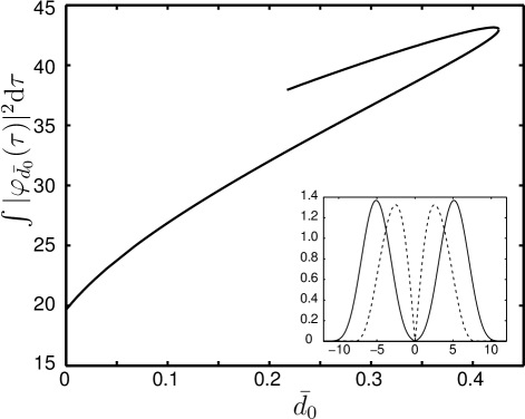
Fig. 1: Bisoliton energy as two valued function of dimensionless residual dispersion $\bar{d_{0}}$. Solid and dashed lines on insert correspond to the upper and lower branch bisolitons with $\bar{d_{0}}=0.256$. Horizontal and vertical axes on insert correspond to dimesionless time and amplitude.

Fig. 1 represents bisoliton energy as function of $\bar{d_{0}}$. Remarkably, this is a multiple valued function with two branches. Calculation of solutions on this second branch required solution of the Arnoldi-Lanczos approximation problem for the linearization of iterration operator. Its limit point is located in the vicinity of $\bar{d_{0}}_{bf}\simeq 0.426$. With all other parameters fixed, smaller values of $\bar{d_{0}}$ correspond to smaller values of residual dispersion. Therefore, the limit point corresponds to the largest value of $d_{0}$ for which bisolitons are supported. According to our calculations, for values of $\bar{d_{0}}>\bar{d_{0}}_{\text{bf}}$ bisolitons will fail to exist and we will only observe a pair of interacting dispersion managed solitons that are not bound, not a bisoliton. The insert to the figure shows that the higher energy bisoliton is wider, with greater separation and broader shape.

Direct numerical simulations demonstrate stability of both the lower and the upper-branch bisoliton solutions over realistic distances (300 periods). For very long propagation distances, the upper branch showed signs of instability. Additionally, the pair of pulses composing the solution tends to stay bound whenever the pulses are pulled apart. The separation between the pulses spread apart in this manner oscillates about the separation for the bisolitonic solution.

In the remainder of this paper, we will discuss the structure of the lower branch solutions. A later paper will present details about the upper branch solutions. The logarithmic density profile of lower branch solutions’ amplitude for a range of values of $\bar{d_{0}}$ is shown in Fig. 2. There lighter shades of gray correspond to a higher value of the amplitude. The black lines correspond to zero values. The dashed lines indicate where the solutions have their maxima. A horizontal slice of this plot gives an amplitude profile for a fixed value of $\bar{d_{0}}$. For example, for a value of $\bar{d_{0}}=0.167$ the logarithm of amplitude is represented on Fig. 3. The dashed line on the same graph represents the result of direct numerical simulations of Eq. (1) after 300 dispersion map periods. A solution of equation 5 provided one boundary condition for this simulation (the launched pulse).

As we see in Fig. 2 bisoliton tails change sign for values of $\bar{d_{0}}<\bar{d_{0}}_{cr}$ ( $\bar{d_{0}}_{cr}\simeq 0.269$ ). As the value of the dimensionless residual dispersion becomes greater than the critical value $\bar{d_{0}}>\bar{d_{0}}_{cr}$, the phase of the tails remains unchanged, and the amplitude approaches an exponentially decaying function.

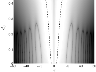
Fig. 2: The contour plot of $\log(|\varphi|)$ as a function of time variable $t$ and a parameter $\bar{d_{0}}$. The dotted lines represents the peak amplitudes of solutions.

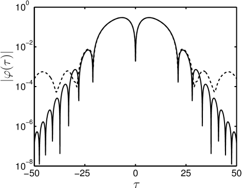
Fig. 3: Intensity profiles of a bisoliton with $\bar{d_{0}}=0.167$: solution of Eq. (5) (solid), and a result of propagation this solution over 300 periods through the line with $s=1.5$, $d_{0}=0.0125$, and $\lambda=0.05$ (dashed)

Our equation Eq. (5) reduces the many physical parameters from Eq. (1)to a single parameter. We have computed the bisolitons for a range of parameter values, and those computed solutions can be used to write solutions of the original physical system

$$u(t,z_{dm}/4+mz_{dm})=\sqrt{\frac{\lambda}{\gamma}}\hat{F}^{-1}\left.\left[\varphi_{\bar{d_{0}}=\frac{d_{0}}{\lambda s}}\left(\Omega\right)\right]\right|_{\tau=t/\sqrt{s}}$$ (7)

where it was convenient to specify the solution at $z_{dm}/4+mz_{dm}$ because it is chirp free at this point.

We use $u(t,z_{dm}/4)$ of Eq. (7) as the initial condition in direct numerical simulation of Eq. (1) to study the dynamics of lower-branch bisoliton solutions for different values of $\bar{d_{0}}$. In particular, we compare temporal-spatial behavior of solutions corresponding to values of $\bar{d_{0}}_{cr}<\bar{d_{0}}<\bar{d_{0}}_{bf}$ and $0<\bar{d_{0}}<\bar{d_{0}}_{cr}$ over a map period. We consider a system with $s=1.5$ and mean dispersion $d_{0}=0.0125$. Fig. 4 and Fig. 4 represent propagation of the initial pulse with $\bar{d_{0}}=0.417$ and $\bar{d_{0}}=0.167$ respectively. For such choices of the system parameters, the values of phase periods $\lambda$ must be 0.05 and 0.02.

The bisolitons for values of $\bar{d_{0}}$ above the critical value have no zeros other than at $\tau=0$ in their unchirped state, while if $\bar{d_{0}}<\bar{d_{0}}_{cr}$ the solution will have an increasing number of zeros with smaller $\bar{d_{0}}$. The example shown in Fig. 4 shows that for larger values of $d_{0}$ the local minima which in part (a) are at $z=0$ split into pairs of minima, which are ”shifted” towards $z_{dm}/2$. In fact, comparing the dynamics of $\bar{d_{0}}=0.417$ and $\bar{d_{0}}=0.167$ bisolitons indicates that the larger the value of $\bar{d_{0}}$ the more the minima will shift from the narrowest states (the valleys) of the pulse to its broadest state (the ridges).

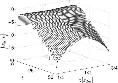
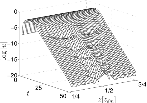
Fig. 4: Waveforms of a logarithm of the amplitude for bisoliton propagation through DM system with $s=1.5$, $d_{0}=0.0125$, $\gamma=1$ (a) $\lambda=0.05$ and (b) $\lambda=0.02$. The soliton magnitude $|u|$ is symmetric. Bisolitons are propagated over half of the period, from $z_{dm}/4$ to $3z_{dm}/4$

In conclusion, we have used a slowly varying stroboscopic equation to calculate bisoliton solutions with well resolved tails. This equation can be rescaled so that it has a single dimensionless parameter $\bar{d}_{0}$. We have found a range of $\bar{d}_{0}$ such that there are two bisoliton solutions for each value of $\bar{d}_{0}$. In addition, the structure of the tails for the lower branch solutions was described in terms of the value of $\bar{d}_{0}$.

We would like to acknowledge many helpful discussions and useful suggestions contributed by M. Stepanov. This work was supported in part by Los Alamos National Laboratory under an LDRD grant, the National Nuclear Security Administration of the U.S. Department of Energy under Contract # DE-AC52- 06NA25396, by the DOE Office of Science Advanced Scientific Computing Research (ASCR) Program in Applied Mathematics Research, as well as Proposition 301 funds from the State of Arizona.

References

- [1] A. Maruta, T. Inoue, Y. Nonaka, and Y. Yoshika, IEEE J. Sel. Top. Quantum Electron. 8, 640 (2002)
- [2] M. Stratmann, T. Pagel, and F. Mitschke, Phys. Rev. Lett. 95 143902 (2005)
- [3] I. Gabitov and S. K. Turitsyn, Opt. Lett. 21, 327 (1996)
- [4] P. M. Lushnikov, Opt. Lett. 26, 1535 (2001)
- [5] L. F. Mollenauer and J. P. Gordon, Solitons in Optical Fibers, (Academic, 2006)
- [6] V. Petviashvili and O. Pokhotelov, Solitary waves in Plasmas and in the Atmosphere (Gordon & Breach) Philadelphia, Pa., 1992, p. 248