Attosecond streaking experiments on atoms: quantum theory versus simple model

Abstract

A new theoretical approach to the description of the attosecond streaking measurements of atomic photoionization is presented. It is a fully quantum mechanical description based on numerical solving of the time-dependent Schrödinger equation which includes the atomic field as well as the fields of the XUV and IR pulses. Also a simple semiempirical description based on sudden approximation is suggested which agrees very well with the exact solution.

One of the problems in the physics of ultrashort atomic phenomena is the characterization of the attosecond extreme ultraviolet (XUV) pulses which are used in pump-probe experiments studying the time evolution of atomic processes. The characterization includes measurements of the pulse duration, intensity, basic frequency, spectral distribution and possible chirp. In a typical experiment Hentschel01 ; Drescher02 ; Kienberger04 ; Goulielmakis04 , the XUV pulses with a duration of a few hundred attoseconds are produced by filtering out the high energy part of the high harmonic spectrum which results from a nonlinear interaction of a few-cycle intense infrared (IR) laser pulse with a gas target. The laser pulse duration is typically 5-7 fs, its carrier wave length is $\sim 800$ nm (the photon energy $E_{L}\sim 1.6$ eV), thus the period of the laser pulse is larger than the XUV pulse duration. The intensity of the laser is typically $3\times 10^{13}-10^{14}$ W/cm². At such intensity the electric field of the laser, ${\cal E}_{L}\sim(0.1-0.3)\times 10^{9}$ V/cm, is much smaller than the atomic field (1 a.u.= 5.14 $\times 10^{9}$ V/cm) although it is strong enough to produce high harmonics. The electric field of the XUV pulse is still smaller, about $7\times 10^{7}$ V/cm Goulielmakis04 , so that the linear response approximation can be readily applied to the interaction of the XUV pulse with atoms. The typical carrier frequency of the XUV pulse corresponds to the photon energy $E_{X}\sim 90$ eV.

The only method of the attosecond pulse characterization, realized up to now, has been the so-called attosecond streak camera Hentschel01 ; Drescher02 ; Kienberger04 ; Goulielmakis04 ; Constant97 ; Itatani02 ; Kitzler02 . The attosecond pulses under investigation ionize atoms of a gas target in the field of a co-propagating IR laser pulse. The bunch of photoelectrons presenting a replica of the XUV pulse interacts with the field of the few-cycle IR pulse. The streaking effect is achieved by measuring the photoelectron yield at different delays between the XUV and laser pulses. The resulting energy and angular distributions of photoelectrons, bearing information on the original attosecond XUV pulse, are measured by methods of electron spectroscopy. Several theoretical methods are used to extract this information from the photoelectron spectra. They are based on the classical equation of motion Itatani02 , the semiclassical approach Itatani02 ; Kitzler02 or quantum mechanical calculations within a strong field approximation Scrinzi01 ; Kitzler02 . In this way, it has been proved that single pulses with a duration of as low as 250 as Kienberger04 and even 150 as Wonisch06 have been produced. The intensity of the XUV pulse has been also measured Goulielmakis04 . In addition, the chirp was demonstrated as being close to zero Kienberger04 . In spite of the obvious success of the streak camera method, there are still many problems in understanding the detailed dynamics of the laser-dressed photoionization of atoms by the ultra-short pulses, the accuracy and limitations of the method. The latter problem has been recently discussed in detail in Ref. Yakovlev05 .

In this Letter we present fully quantum mechanical calculations of the double differential cross section of atomic photoionization by an ultrashort XUV pulse in the presence of a few-cycle intense IR pulse. The results provide complete information about the process which may be used either for comparison with an experiment or as a test-ground for approximate models. We present also a simple model which permits us to produce a quick analysis of the experimental data and to study the sensitivity of the measurements to the parameters of the attosecond pulses.

The photoelectron spectra and angular distributions are calculated by solving the time-dependent Schrödinger equation numerically. The atom is described by the independent-electron model, and we assume that the orbitals of all electrons except the active one are frozen. This approximation is valid for not very strong laser fields ( ${\cal E}_{L}\ll 1$ a.u.). We suppose that both IR and XUV photons are linearly polarized and their polarization vectors are parallel. In this case there is an axial symmetry with respect to the axis of polarizations which we choose as $z$-axis. By expanding the active electron wave function in spherical harmonics

$$\psi(\vec{r},t)=\sum_{\ell=0}^{L_{\max}}u_{\ell}(r,t)Y_{\ell 0}(\theta,\varphi)$$ (1)

and substituting the expansion into the time-dependent Schrödinger equation we obtain the following set of equations for the coefficient functions $u_{\ell}(r,t)$

$$i\frac{\partial}{\partial t}u_{\ell}(r,t)=-\frac{1}{2}\frac{\partial^{2}}{\partial r^{2}}u_{\ell}(r,t)+\left[U_{\ell}(r)+\frac{\ell(\ell+1)}{2r^{2}}\right]u_{\ell}(r,t)$$

$$+r{\cal E}_{L}(t)\sum_{\ell^{\prime}=0}^{L_{\max}}C(\ell,\ell^{\prime})u_{\ell^{\prime}}(r,t)$$

$$+\frac{1}{2}rC(\ell,\ell_{0})\delta_{\ell,\ell_{0}\pm 1}\bar{\cal E}_{X}(t)\exp[-i(\omega_{X}+\varepsilon_{0})t]u_{\ell_{0}}(r).$$ (2)

Here and in the following atomic units are used unless otherwise indicated. In Eq. (2) $U_{\ell}(r)$ is a single electron potential, $C(\ell,\ell^{\prime})$ is the angular part of the dipole matrix element, $\varepsilon_{0}$ is the binding energy of the active electron, ${\cal E}_{L}(t)$ is an electric field of the laser pulse while $\bar{\cal E}_{X}(t)$ is an envelope of the XUV pulse. Since the XUV field is weak, the first order perturbation theory and the rotating wave approximation are applied. Then in the dipole approximation, only transitions $\ell_{0}\rightarrow\ell_{0}\pm 1$ are possible. In contrast, the laser IR field is strong, it mixes the states with different orbital angular momenta. In order to achieve sufficient accuracy, the partial waves up to $L_{max}\sim 40-60$ have been included.

The system of equations (2) has been solved numerically using the split-propagation method. The details of the numerical procedure will be published elsewhere (see also Refs. Kazan05 ; Kazan06 ). Calculating the set of the functions $u_{\ell}(r,t)$ at $t\to\infty$ we have evaluated the partial amplitudes of photoionization by projecting the functions onto the corresponding continuum functions $\chi_{-}^{(\ell)}(E;r)$:

$${\cal A}_{\ell}(E)=\exp[i\eta_{\ell}(E)]\int_{0}^{\infty}dru_{\ell}(r,t\to+\infty)\chi_{-}^{(\ell)}(E;r),$$ (3)

where $\eta_{\ell}(E)$ is the photoionization phase (for details see Ref. Kazan06a ). Knowing the amplitudes, ${\cal A}_{\ell}(E)$, one can evaluate the double differential cross section (DDCS)

$$\frac{d^{2}{\sigma}(E,\Omega)}{dEd\Omega}=2\pi\omega_{X}\alpha K^{-1}\left|\sum_{\ell}{\cal A}_{\ell}(E)Y_{\ell 0}(\vartheta)\right|^{2}\,.$$ (4)

Here $\alpha$ is the fine-structure constant and $K=\int dt|\bar{\cal E}_{X}(t)|^{2}$. By integrating Eq. (4) over the emission angle one can obtain the photoelectron spectrum.

As an example we consider the 3s subshell photoionization in Ar. The atom is described within the Hartree-Slater approximation HS78 with the same self-consistent potential $U(r)$ for each $\ell$. The laser pulse is assumed to have the form

$${\cal E}_{L}(t)=\bar{\cal E}_{L}(t)\cos{[\omega_{L}(t-\tau_{L})+\phi_{L}]}$$ (5)

with the envelope given by the expression

$$\bar{\cal E}_{L}(t)={\cal E}_{L0}\frac{1}{2}\{\cos[\pi(t/\tau_{L}-1)]+1\}\,,$$ (6)

where $\tau_{L}$ gives the full width at half maximum (FWHM) and $\phi_{L}$ is the carrier-envelope phase. We set $\phi_{L}=0$ (cosine-type pulse).

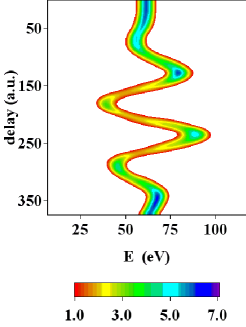
Figure 1: (Color online) A 2D plot of the Ar(3s) photoelectron spectra (electron energy - x-axis) at $0^{\circ}<\vartheta<15^{\circ}$ as a function of the time delay in a.u. (1 a.u. = 24.2 as) between the laser and the XUV pulses (y-axis). The calculations were performed for the IR pulse of the cosine-type with the duration $\tau_{L}=5.0$ fs, the laser intensity is 10¹³ W/cm². The XUV pulse duration is $\tau_{X}=250$ as and the carrier frequency is 90 eV. The calculated binding energy of Ar(3s) is 28.6 eV

The XUV pulse is delayed with respect to the laser pulse by $t_{d}$

$${\cal E}_{X}(t)=\bar{\cal E}_{X}(t-t_{d})\cos{[\omega_{X}(t-t_{d})]}\,.$$ (7)

For the envelope $\bar{\cal E}_{X}(t)$ we have chosen the hyperbolic secant shape. The parameters of the laser and the XUV pulses are shown in the caption to Fig. 1. This figure shows the two-dimensional (2D) plot of the calculated spectra as a function of the delay between the laser and the XUV pulses. The results shown in Fig. 1 are typical for the streaking experiment Drescher02 ; Kienberger04 ; Goulielmakis04 .

If the duration of the XUV pulse is much shorter than the period of the laser field, $\tau_{X}\ll T_{L}$, then one can consider the whole process as a two-step one Itatani02 : first step is photoionization of the atom by the XUV pulse which is independent of the laser field, second step is a transport of the emitted electron by the laser field to the final state. Within the linear response approximation, the cross section of photoionization by a short pulse (without the IR field) can be presented as Kazan06a

$$\frac{d\sigma_{0}}{d\vec{p}_{0}}=\frac{a}{\sqrt{2E_{0}}}\left|D(E_{0})\right|^{2}\left|f(E_{0}+|\varepsilon_{0}|-\omega_{X})\right|^{2}Y_{10}^{2}(\vartheta_{0})\,.$$ (8)

Here $\vec{p}_{0}$ is the linear momentum of the photoelectron immediately after photoionization ($\vartheta_{0}$ is the corresponding emission polar angle, $E_{0}$ is the electron energy), $D(E_{0})$ is the dipole matrix element for transition to the continuum state with the energy $E_{0}$,  $f(\epsilon)$  is the Fourier transform of the XUV pulse at the energy $E_{0}+|\epsilon_{0}|$, and $a=2\pi\omega_{X}\alpha K^{-1}$. The factor $Y_{10}^{2}(\vartheta_{0})$ describes the angular distribution of photoelectrons for the particular case of the s$\to$p transition considered here.

With the IR field, the cross section modifies as follows

$$\frac{d\sigma}{\sqrt{2E}dEd\Omega}=\frac{d\sigma}{d\vec{p}}=\frac{d\sigma_{0}}{d\vec{p}_{0}}\left|\frac{\partial(\vec{p}_{0})}{\partial(\vec{p})}\right|,$$ (9)

where $\vec{p}$ is the final momentum of the electron, $\left|\frac{\partial(\vec{p}_{0})}{\partial(\vec{p})}\right|$ is the transformation determinant. Now we are to link the variables $(\vartheta_{0},E_{0})$ with the experimentally observable quantities $(\vartheta,E).$  The basic relations for the components of the momentum $\vec{p}\equiv\{p_{\parallel},p_{\perp}\}$ parallel and perpendicular to the field are

$$p_{\parallel}=p_{0\parallel}-\int_{\tau}^{\infty}{\cal E}_{L}(t)~{}dt\equiv p_{0\parallel}-A_{L}(\tau),$$ (10)

$$\quad p_{\perp}=p_{0\perp},$$ (11)

from which it follows $\left|\frac{\partial(\vec{p}_{0})}{\partial(\vec{p})}\right|=1$ and

$$\sin\vartheta_{0}=\sqrt{E/E_{0}}\sin\vartheta\,.$$ (12)

Here $\tau$ is the time of the photoelectron emission and $A_{L}(\tau)$ is a parallel component of the vector potential of the laser field in the Coulomb gauge. From Eqs. (10) and (12) it follows that

$$E_{0}=E+\sqrt{2E}A_{L}(\tau)\cos\vartheta+A_{L}^{2}(\tau)/2.$$ (13)

The final approximate expression for the DDCS reads:

$$\frac{d\sigma}{dEd\Omega}=a\,\sqrt{\frac{E}{E_{0}}}\left|D(E_{0})\right|^{2}\left|f(E_{0}+|\varepsilon_{0}|-\omega_{X})\right|^{2}Y_{10}^{2}(\vartheta_{0})\,,$$ (14)

where $E_{0},\vartheta_{0}$ and $E,\vartheta$ are connected by Eqs. (13, 12).

In Fig. 2(a) we compare the DDCS calculated by the numerical solution of the Schrödinger equation and by using Eq. (14) in the case when the delay time is 7 fs.

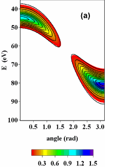
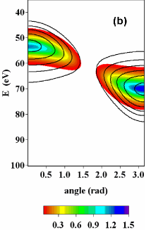
Figure 2: (Color online) 2D plots of the calculated DDCS for Ar(3s) photoionization for different time delays between the laser and the XUV pulses: (a) $t_{d}=290$ a.u. (7 fs), (b) $t_{d}=270$ a.u. (6.5 fs). The parameters of the pulses are the same as in Fig. 1. Contour plots show the results obtained by solving the Schrödinger equation; color (grey) scale plots show the results of model calculations using Eq. (14). The minimal and maximal values are the same for both plots.

The agreement between the two calculations is almost perfect. Note that at the chosen delay ${\cal E}_{L}(t_{d})$ is almost zero. Similar agreement is obtained for all other delays when the laser field is close to zero. In contrast, for the case of $t_{d}=6.5$ fs shown in Fig. 2(b), the distribution given by the exact computation is substantially broader than that given by the approximate formula. Similar discrepancy is obtained for other delays when the value of the laser field is close to its extrema.

From the angular distributions calculated for each time delay we obtain the photoelectron energy spectra at a given angle by integrating over some acceptance angle ($15^{\circ}$) of the detector. These spectra are fitted with the Gaussian function $A\,\exp[-(E-\bar{E})^{2}/\Gamma^{2}]$ in order to determine their widths. Variation of the spectral width with the time delay is commonly used in order to determine the parameters of the XUV pulses Hentschel01 ; Kienberger04 . In Fig. 3 we show the widths $\Gamma$ of the calculated spectra as a function of the delay time for two angles $\vartheta=0^{\circ}$ and 180^∘. Comparing the results of the exact calculations (symbols) with the calculations using the approximate formula Eq. (14) (dotted curves) we have noticed that the difference is always proportional to the value of the IR laser electric field at the moment of the photoelectron emission. As is known Itatani02 , the broadening of the electron spectra (for electrons emitted in the same direction) is determined by two factors. First, the spectrum becomes broader since the emitted electrons have different energies due to the large spectral width of the XUV pulse. This type of broadening is taken into account by Eqs. (13) and (14). Second, the electrons are emitted at different times within the XUV pulse duration and, therefore, at slightly different phases of the IR field that leads to an additional spread of the electron energies. Since $\tau_{X}\ll T_{L}$, this spread depends linearly on the field at the moment of electron emission, and in the first approximation it is proportional to the duration of the XUV pulse. Thus we suggest a semiempirical expression for the width:

$$\Gamma=\Gamma_{m}+\sqrt{2E_{0}}{\cal E}_{L}(t_{d})\tau_{1/2}/2\,,$$ (15)

where $\Gamma_{m}$ is a model width, calculated from the spectra obtained using Eq. (14) and $\tau_{1/2}$ is a FWHM of the XUV field envelope. Using this expression we obtained the values, shown by solid lines in Fig. 3, which are in excellent agreement with the results of the exact calculations shown by open symbols, circles (forward emission) and squares (backward emission).

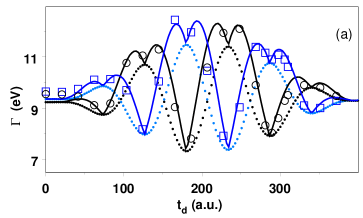
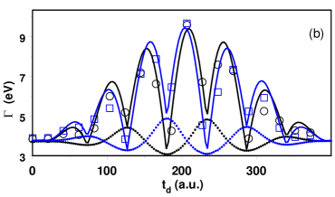
Figure 3: (Color online) The width of the photoelectron spectrum as a function of the delay time for two XUV pulse durations: (a) $\tau_{X}=100$ as, (b) $\tau_{X}=250$ as. Black symbols and curves correspond to forward emission $\vartheta=0^{\circ}$, blue (gray) symbols and curves correspond to backward emission $\vartheta=180^{\circ}$. Exact calculations: circles ($\vartheta=0^{\circ}$) and squares ($\vartheta=180^{\circ}$). Dotted curves show $\Gamma_{m}$ obtained by model calculations. Solid curves show the results obtained by Eq. (15). All parameters in the calculations are the same as in Fig. 1.

Besides very good agreement between the calculations, an interesting feature can be seen in Fig. 3, namely a double-maximum structure in the resulting model curve for the pulse duration of 100 as. This is not an artefact since the exact calculations with small steps in time delay around $t_{d}=300$ a.u. perfectly agree with the model calculations. The structure is due to the fact that at the zero-crossing points where ${\cal E}_{L}(t_{d})=0$, the width should be equal to that obtained from Eq. (14), and therefore a minimum is formed. The depth of the minimum is determined by the contribution of the pulse spectral width (dotted curve). For longer pulses (250 as) this contribution is smaller and the minimum is deeper. An analysis of the results obtained with model expression Eq. (14) shows that for very short XUV pulses ( $\leq$ 100 as) the model describes the width quite well, as well as describing the whole structure of the DDCSs. Thus, for such short pulses one can keep track only on the spectrum of the XUV pulse but not on its duration and the chirp. With an increase of the XUV pulse duration, the first term in Eq. (15) is decreasing while the second one is increasing and becomes dominant. The second term gives information on the FWHM of the XUV envelope. The latter quantity can also depend on the chirp, although this dependence is not strong. Thus, the chirp can be obtained only for the pulses for which the second term in Eq. (15) is sufficiently large. The value of this term is proportional to the strength of the IR field and to the duration of the XUV pulse. Thus stronger IR fields and longer XUV pulse durations are favorable for chirp registration.

In conclusion, we have developed a fully quantum mechanical theory of the streaking measurements in the attosecond region based on numerical solving of the time-dependent Schrödinger equation which includes the electron interaction with the atomic core as well as with the XUV and the laser fields. We suggest also a simple model expression for the width of the photoelectron spectra which agrees very well with the exact calculations. Using this expression it is easy to analyze the sensitivity of the width to the parameters of the XUV pulse.

The financial support from the Russian Foundation for Fundamental Research via Grants 05-02-16216 and 06-02-16289 is gratefully acknowledged.

References

- (1) M. Hentschel, R. Kienberger, Ch. Spielmann, G. A. Reider, N. Milosevic, T. Brabec, P. Corkum, U. Heinzmann, M. Drescher, and F. Krausz, Nature 414, 509 (2001).
- (2) M. Drescher, M. Hentschel, R. Kienberger, M. Uiberacker, V. Yakovlev, A. Scrinzi, Th. Westerwalbesloh, U. Kleineberg, U. Heinzmann, and F. Krausz, Nature 419, 803 (2002).
- (3) R. Kienberger, E. Goulielmakis, M. Uiberacker, A. Baltuska, V. Yakovlev, F. Bammer, A. Scrinzi, Th. Westerwalbesloh, U. Kleineberg, U. Heinzmann, M. Drescher, and F. Krausz, Nature 427, 817 (2004).
- (4) E. Goulielmakis, M. Uiberacker, R. Kienberger, A. Baltuska, V. Yakovlev, A. Scrinzi, Th. Westerwalbesloh, U. Kleineberg, U. Heinzmann, M. Drescher, and F. Krausz, Science 305, 1267 (2004).
- (5) E. Constant, V. D. Taranukhin, A. Stolow, and P. B. Corkum, Phys. Rev. A 56, 3870 (1997).
- (6) J. Itatani, F. Quéré, G. L. Yudin, M. Yu. Ivanov, F. Krausz, and P. B. Corkum, Phys. Rev. Lett. 88, 173903 (2002).
- (7) M. Kitzler, N Milosevic, A. Scrinzi, F. Krausz, and T. Brabec, Phys. Rev. Lett. 88, 173904 (2002).
- (8) A. Scrinzi, T. Brabec, and M. Walser, Proceed. Workshop on Super-Intense Laser-Atom Physics, p. 313 (2001).
- (9) A. Wonisch, U. Neuhäusler, N. M. Kabachnik, T. Uphues, M. Uiberacker, V. Jakovlev, F. Krausz, M. Drescher, U. Kleineberg, and U. Heinzmann, Applied Optics 45, 4147 (2006).
- (10) V. S. Yakovlev, F. Bammer, and A. Scrinzi, J. Mod. Opt. 52, 395 (2005).
- (11) A. K. Kazansky and N. M. Kabachnik, Phys. Rev. A 72, 052714 (2005).
- (12) A. K. Kazansky and N. M. Kabachnik, J. Phys. B 39, L53 (2006).
- (13) A. K. Kazansky and N. M. Kabachnik, Phys. Rev. A 73, 062712 (2006).
- (14) F. Herman and S. Skillman, Atomic Structure Calculations (Prentice-Hall, Englewood Cliffs, NJ, 1963).