Maxwell demon in Granular gas: a new kind of bifurcation? The hypercritical bifurcation

Abstract

This paper starts with the investigation of the behaviour of a set of two subsystems which are able to exchange some internal quantity according to a given flux function. It is found that this sytem exhibit a bifurcation when the flux passes through a maximum and that its kind (super-critical/sub-critical) depends on the dissymmetry of the flux function near the maximum. It is also found a new kind of bifurcation when the flux function is symmetric: we call it hypercritical bifurcation because it generates much stronger fluctuations than the super-critical one. The effect of a white noise is then investigated. We show that an experimental set-up, leading to the Maxwell demon in granular gas, displays all these kinds of bifurcation, just by changing the parameters of excitation. It means that this system is much less simple as it was thought.

I Introduction

The theory of dynamical systems is a general field of research which has many applications in different areas, including fluid dynamics drazin97 , population dynamics murray02 or chemical reaction mei00 among others. The idea of this field is to connect physical problems which are completely different and which pertain in different areas, just because they are driven by a similar set of equations. Due to this, a solution obtained in one case can be applied to the other domains, just by settling the analogy. But to be correct, the method requires to settle the correct analogy, i.e. the correct change of variables and boundary conditions, which needs in turn some rigour. One of the key issue in these problems is the determination of the stationary states, their stability (attractors), the dimension of the stable subspace … Also one can ask how the solutions evolve when applying different constrains on the system. This means to study the variation of the set of attractors as a function of external conditions to determine some possible bifurcation. The way to proceed is well known and it is possible to characterise the transition between different stationary states thanks to the bifurcation theory crawford91 ; pomeau ; manneville . This latter allows to describe the dependence of a stationary state with respect to some experimental parameters for instance. It has then been pointed out that a single stationary state may evolve to two or more stationary states as a control parameter changes. This has led to study the well-known (super-)critical and sub-critical bifurcations for instance. However, it is also possible that a stationary state evolves and splits into a continuous set of stationary states but this has not been studied yet. Nevertheless, as we demonstrate in this paper with a specific and simple example, this latter kind of bifurcation. We will even show experimentally a simple example where all these different types of bifurcations can occur, i.e. super-critical and sub-critical, plus the hypercritical one. In this case, this last one will occur when the system jumps from one kind of bifurcation to the other kind. We will firstly present the theoretical approach. Then we will present the classical experiment of the “Maxwell demon in granular gas”. And we will prove that this experiment can be used to study all these three type of bifurcation. In turn, it demonstrates that this experiment is much less simple than it was thought, and that the published explanations are not complete.
We will start the paper with the theoretical analysis. To simplify the concepts, we consider a system made of two point-like subsystems exchanging a part of some physical quantity. This quantity is an internal property of extensive nature. And we investigate its dynamics. We will focus on a case where the exchange is driven by the flux functions of each subsystems. Each flux function will be assumed to depend only on the content of each subsystem (i.e. it does not depend on the other subsystem).
When both subsystems are submitted to the same external conditions, one expects that both flux functions are identical. A steady state corresponds to an equilibrium state if it is stable. When the flux function has a maximum, multiple equilibrium states can exist. So, a bifurcation occurs when the control parameter allows the flux to evolve and pass through the maximum. The kind of bifurcation depends drastically on the shape of the flux curve. We will see that a new kind of bifurcation, called hypercritical, can be found with some special constraints on the shape of the flux function. It corresponds to the case when a unique attractor degenerates into a subspace of dimension $d_{A}$ larger than $0$. This generates an indeterminacy at some precise value of the constrains. Apart from this precise constrain, either a single attractor or a set of two attractors exist. The case which will be studied here is the case $d_{A}=1$ but larger dimension of subset could be envisaged ($d_{A}=2,3$) or fractal subsets too $d_{A}>0$. Most of the analysis will use a continuum approach. However, at the end of the theoretical part the effect of noise will be introduced; this one can be due to the ”granular” nature of the extensive quantity. When this noise is taken into account, the kind of bifurcation is particularly ticklish to display and the set of the two subsystems undergoes a diffusion-like process, which may be solved using a Langevin’s formalism. This diffusion process may broaden the ”point-like” attractor when the attractor is unique, or when the attraction of the attractors is large compared to the noise agitation when there are more than one attractor. In this case the steady state expands over a given volume of the phase space. But the noise can also generate repeated jumps between the set of attractors when attractors are discrete in this last case, or even provoke a diffusion among a continuous or discrete set of possible attractors. All these configurations will be considered.

In the last part, the paper will revisit the problem of the Maxwell’s demon in granular matter, which can be stated as follows: consider two halve-containers containing few grains each and connected by a lateral hole. The system is vibrated and the grains are agitated so that they can pass from one container to the other one alternately. In practise one should expect an equi-repartition. However this one is ensured only when the vibration excitation is large enough, but when the excitation becomes two small and the dissipation is large enough, one observes that a container is more filled than the other. This occurs because the larger dissipation in the more filled container reduces the agitation of the grains and the probability of these ones to escape, while the smaller dissipation in the second container increases the speed of the grains in this box and favoured the transfer to the other box. The present experiment will use a single vibrated container containing some grains, and in which a hole has been drilled on a side to allow grains to escape. This will allow to measure the flux function J of grains going out from the box as a function of the number N of grains in the container. We will see that the measured flux functions let predict the existence of an hypercritical bifurcation for some range of parameters. As this result was not found by previous experiments, numerical simulations and theoretical approaches, it proves that the problem was not properly settled and that the correct equations are still not given. This proves that much work remains to be performed on granular materials and that much care has to be taken to settle correct analogies.

The paper is built as follow: Section II presents the general issue, the equations which rule the evolution of the system and the equilibrium condition for which the internal quantity in each subsystem remains constant. Section III presents an analysis of the bifurcation problem occurring when the internal quantity maximises the flux function. The hypercritical bifurcation is defined and the condition of its occurrence characterised. The effect of noise is also discussed. Finally, section IV is devoted to a convenient experiment to study the so called “Maxwell’s demon phenomenon in granular matter” presented above. The paper is concluded in section V.

II Preliminaries

Consider two subsystems, left and right ($l$, $r$), each characterised by an internal extensive quantity, $x_{l}$ and $x_{r}$ and submitted to a set of external conditions, $y_{l}^{(i)}$ and $y_{r}^{(i)}$. We assume first that the set of the two subsystems is closed such that:

$$x_{r}+x_{l}=x_{tot}=2x_{0}=cste.$$ (1)

Also the exchange between the two subsystems is ruled thanks to two flux functions, $J_{l}$ and $J_{r}$ associated to each subsystem. These flows are assumed to depend on the external parameters, $y_{l}^{(i)}$ or $y_{r}^{(i)}$, applied to each container and on its content $x_{l}$ or $x_{r}$ only. Thus, this paper aims at describing the evolution of such subsystems, at finding if stationary or equilibrium states exist, if they are stable (equilibrium states) or not and at studying the possibility of exhibiting some bifurcations when external parameters, $y_{l}^{(i)}$ or $y_{r}^{(i)}$, evolve.

As an example, one can consider the “granular Maxwell demon” schlichting96 ; eggers99 where two containers connected by a slit are vibrated. These containers are partially filled with macroscopic particles and can exchange some particles across the slit. Here, the internal quantities are the number of particles in each box while the external conditions are the dimension of each box, the position and size of the slit, the frequencies and amplitudes of vibration for each box, the gravity and so on. In this peculiar case, it is known that particles equipartition is observed for intense enough vibration, but that it breaks at small enough vibration excitation, displaying a threshold and a bifurcation.

Coming back to the more general case, the time evolution of the system is given by the time evolution of $x_{l}$ and $x_{r}$ which writes:

$$\frac{dx_{l}}{dt}=J_{r}(x_{r})-J_{l}(x_{l}).$$ (2)

And equation (1) imposes:

$$\frac{dx_{r}}{dt}=-\frac{dx_{l}}{dt}.$$ (3)

Both subsystems are stationary (and then in equilibrium but not always stable) if $\frac{dx_{l,r}}{dt}=0$, which imposes in turn that their flux are equal:

$$J_{l}(x_{l})=J_{r}(x_{r}).$$ (4)

One has now to determine whether this steady/equilibrium state ($x_{l,0}$, $x_{r,0}$) is stable or not. It is stable if any small perturbation $\delta x$ of $x_{l,0}$ and $x_{r,0}$ (i.e. $x_{l}=x_{l,0}+\delta x$ and $x_{r}=x_{r,0}-\delta x$) decreases spontaneously with time. It is unstable on the contrary. A first order expansion gives:

$$\frac{d(x_{l,0}+\delta x)}{dt} = J_{r}(x_{r,0}-\delta x)-J_{l}(x_{l,0}+\delta x),$$ (5)

$$\Rightarrow\frac{d\delta x}{dt} \approx -\delta x\left[\frac{dJ_{r}}{dx}(x_{r,0})+\frac{dJ_{l}}{dx}(x_{l,0})\right],$$ (6)

$$\Rightarrow\frac{d\delta x}{dt} \approx -\alpha\delta x.$$ (7)

Where $\alpha=\frac{dJ_{r}}{dx}(x_{r,0})+\frac{dJ_{l}}{dx}(x_{l,0})$. Consequently, a steady/equilibrium state is stable when $\alpha>0$ and unstable when $\alpha<0$.

For the sake of simplicity, we will limit hereafter the formulation to two systems with some symmetries, but generalisation is straightforward. So, we will assume that both systems are identical (same size, slit at the same position, …) and are submitted to equivalent external conditions. It means in particular that $J_{l}$ and $J_{r}$ depend only on $x_{l}$ and $x_{r}$ respectively and on a unique set of external conditions. This imposes also that $J_{l}(x)=J_{r}(x)=J(x)$.
One would like now to know if a stable equilibrium state can become unstable when varying a control parameter. This leads to determine under which condition a bifurcation could occur and which kind of bifurcation could be obtained from this formalism.

III Bifurcation Analysis

III.1 Classical analysis

Let us assume that the two subsystems contain both $x_{0}$ initially. From equation (3) and according to equation (4), as soon as the two subsystems are identical and are submitted to the same constrains, the state defined by $x_{l}=x_{r}=x_{0}$ is a steady state. According to equation (7), this state remains stable as long as the first derivative of $J$ at $x_{l/r}$ is positive that is, as long as $J$ increases with $x$ at $x_{0}$. This solution becomes unstable as soon as $J$ starts decreasing. In this case, a new solution has to be found which satisfies $x_{l}+x_{r}=2x_{0}=cste$ and $J(x_{l})-J(x_{r})=0$. This is the jump from the unique solution to the set of two different solutions which will interest us during this section. It occurs when $dJ/dx$ passes through $0$.

Generally, as $J$ is an outgoing flux, one expects that $J$ increases at small $x$ starting from $J(0)=0$. So, the jump/bifurcation occurs when $J$ passes through a maximum. However, it may occurs that $J$ starts from a non null value and passes through a minimum in some cases but the analysis is similar to the one made in the following when $J$ increases at small $x$.
Note also that we will consider in this paper only the flux function for which the first derivative could cancel at most one time and the case where $J$ is infinitely derivable.

So, turning back to the most probable case for which $J$ increases at small enough $x$, i.e. $\frac{dJ}{dx}>0$ at small $x$, it means that a transition occurs when the flux function reaches its maximum value $J(x_{m})$. This leads to study and determine the kind of bifurcation which occurs around $x_{l,r}=x_{m}$. The parameter $v$ which controls the distance to the threshold is $v=x_{l}+x_{r}-2x_{m}$ and can be used to study the bifurcation nature. In this case, the preserved quantity $x_{l}+x_{r}$ writes $x_{l}+x_{r}=2x_{m}+v$. It is also convenient to introduce the asymmetry parameter $u=x_{l}-x_{r}$ as the order parameter. So writing $J$ as a function of the distance to the maximum and using a Taylor expansion, one obtains:

$$J(x_{l}-x_{m}) = J(x_{m})+\sum_{k=1}^{\infty}\frac{(x_{l}-x_{m})^{k}}{k!}\frac{d^{k}J}{dx^{k}}(x_{m}),$$

$$J(x_{r}-x_{m}) = J(x_{m})+\sum_{k=1}^{\infty}\frac{(x_{r}-x_{m})^{k}}{k!}\frac{d^{k}J}{dx^{k}}(x_{m}).$$ (8)

We use the notation hereafter $J^{(k)}(x_{m})=\frac{d^{k}J}{dx^{k}}(x_{m}$. By hypothesis, $J^{(2)}(x_{m})=\frac{d^{2}J}{dx^{2}}(x_{m})<0$ and $J^{(1)}(x_{m})=\frac{dJ}{dx}(x_{m})=0$ is the bifurcation threshold.

So, using the change of variable:

$$\frac{u+v}{2} = x_{l}-x_{m},$$ (9)

$$\frac{v-u}{2} = x_{r}-x_{m}.$$ (10)

The dynamics equations becomes at third order:

$$\frac{du}{dt} = -u\left(vJ^{(2)}(x_{m})+\frac{v^{2}}{4}J^{(3)}(x_{m})+...\right)$$

$$-u^{3}\left(\frac{1}{12}J^{(3)}(x_{m})+...\right)+...$$

$$\frac{dv}{dt} = 0.$$ (11)

$J^{(1)}(x_{m})=0$ and $J^{(2)}(x_{m})<0$ by hypothesis.
The solution of equations (11) at first order is:

$$u(t)\sim\exp{-(vJ^{(2)}(x_{m})t)}.$$ (12)

As $J^{(2)}(x_{m})<0$, the solution defined by equation (12) is stable for $v<0$ and unstable for $v>0$ and one deduces the typical time $\tau$ of evolution $\tau=\left(vJ^{(2)}(x_{m})\right)^{-1}$. It is worth noting that $\tau$ tends to infinity as $v$ tends to $0$. This is the so-called “critical slowing down” and it means that the equilibrium needs an infinite time to be reached. To get the correct time behaviour at $v=0$, one shall expand equation (11) to higher order in $u$. This leads to a power law relaxation instead of an exponential one.

A stationary state corresponds to $\frac{du}{dt}=0$. Thus, a solution to equation (11) with $\frac{du}{dt}=0$ is:

$$u = 0.$$ (13)

As already told, this solution is stable if $v<0$ and unstable if $v>0$. It means that $x_{l}=x_{r}$ is a stable equilibrium state as long as $x_{l}+x_{r}<2x_{m}$. So, when $v>0$ the solution $u=0$ is unstable. To get the behaviour, one has to take account for higher order term in the development.

III.1.1 Case $J^{(1)}(x_{m})=0$, $J^{(2)}(x_{m})<0$, $J^{(3)}(x_{m})>0$

Limiting to the third order, this gives two new solutions for equation (11) when $J^{(3)}(x_{m})>0$ and $v>0$:

$$u_{\pm} = \pm\left(-v\frac{J^{(2)}(x_{m})+...}{\frac{1}{12}J^{(3)}(x_{m})+...}\right)^{1/2},$$ (14)

$$= \pm\sqrt{\mu}.$$

One can show that these solutions are stable. As the two new solutions do not exist at $v<0$, the bifurcation is the one described in figure 1, with a parabolic branching at $v>0$. This is characteristic of a super-critical fork bifurcation (because the new solutions are stable). In the present case, it occurs at $J^{(1)}(x_{m})=0$, with $J^{(2)}(x_{m})<0$ and $J^{(3)}(x_{m})>0$.

The two solutions appear also when $J^{(3)}(x_{m})>0$ and $v<0$ but this case will be studied later. Let us simply mentioned that they are unstable.

To conclude with the case $\{J^{(1)}(x_{m})=0,J^{(2)}(x_{m})<0,J^{(3)}(x_{m})>0\}$, when $v$ increases from $v<0$ to $v>0$, the solution $x_{l}=x_{r}$ then breaks following a super-critical bifurcation with two symmetric and stable solutions $u_{\pm}$ shown on Figure 1. Figure 2 shows a typical shape of $J$ when $J^{(2)}(x_{m})<0$ and $J^{(3)}(x_{m})>0$. It is characterised by a left wing steeper than the right wing. This allows the $x$ position of the middle of an horizontal secant at given $J$ to increase as $J$ decreases, which is the requirement to get the super-critical bifurcation. Indeed, in the case $2x>2x_{m}$, any steady solution above $x_{m}$ requires to find two solutions $x_{1}$ and $x_{2}$, such as $J(x_{1})=J(x_{2})$ and $x_{1}+x_{2}=2x>2x_{m}$. Such a possibility exists only if the middle of the horizontal secant at a given $J$ increases when $J$ decreases. This is also what $J^{(3)}(x_{m})>0$ means when $J^{(1)}(x_{m})=0$ and $J^{(2)}(x_{m})<0$.

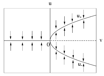
Figure 1: Solutions of equations (11) for $J^{(3)}(x_{m})>0$. Full lines show the stable solution while dashed line shows the unstable ones. Arrows describe the time evolution of a perturbation $\delta u$. Super-critical bifurcation when $v$ becomes positive.

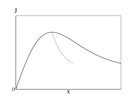
Figure 2: An example of the shape for $J$ corresponding to a super-critical bifurcation (i.e. with $J^{(3)}(x_{m})>0$). The right wing shall be broader than the left wing. The dashed line is the location of the middle of horizontal secant.

III.1.2 Case $J^{(1)}(x_{m})=0$, $J^{(2)}(x_{m})<0$, $J^{(3)}(x_{m})<0$

When $J^{(3)}(x_{m})<0$, there is no solution to equation (11) with $\frac{du}{dt}=0$ for $v>0$. This is due to the fact that the position $x_{mid}$ of the middle of the secant at a given $J$ increases with $J$ when the right wing of the $J$ curve is steeper than the left one, as it is exemplified in Figure 4. So, to get a solution one shall expand equation (8) at higher order in the vicinity of $v=0$ in equation (2). Furthermore, owing to the fact that the dynamics of the system is controlled by the subtraction of two flows, the $u^{4}$ term cancels (as the $u^{2}$ term had disappeared in equation (11)) and one shall develop to fifth order.

Using the change of variable ((9) and (10)) and applying these expansions lead to the following dynamics equation:

$$\frac{du}{dt} = -u\left(vJ^{(2)}(x_{m})+\frac{v^{2}}{4}J^{(3)}(x_{m})+\frac{v^{3}}{24}J^{(4)}(x_{m})+\frac{v^{4}}{192}J^{(5)}(x_{m})+...\right)$$ (15)

$$-u^{3}\left(\frac{1}{12}J^{(3)}(x_{m})+\frac{v}{24}J^{(4)}(x_{m})+\frac{v^{2}}{96}J^{(5)}(x_{m})+...\right)$$

$$-u^{5}\left(\frac{1}{960}J^{(5)}(x_{m})+...\right)+...$$

A possible stationary state ($\frac{du}{dt}=0$) of equation (15) is $u=0$ but it is only stable if $v<0$ in the vicinity of $v=0$. It is unstable for $v>0$. The other possible solutions are symmetric compared to $u=0$. Furthermore, equation (15) with $\frac{du}{dt}=0$ accepts three solutions when $v>0$ (two stable and one unstable), five solutions in the range $v\in[v_{min}<0;0]$ (three stable and two unstable) and one stable solution when $v<v_{min}$.

A typical example of such a case is displayed on Figure 3. An example of curve $J$ corresponding to this bifurcation is displayed on Figure 4. It is characterised by a right wing steeper than the left wing, as explained previously, and by the position $x$ of the middle of a horizontal secant that increases when $J$ increases beyond a value depending on its shape.

So, when $v<v_{min}$, $u=0$ is the only (stable) solution. Then, when $v\in[v_{min}<0;0]$, the solution $u=0$ remains stable but there are also two other stable solutions, both are separated from the $u=0$ solution by an unstable solution. This is typical of multistable state, which is known to lead to hysteresis. When $v>0$, $u=0$ is now an unstable solution and the two symmetric solutions $u_{\pm}$ are the two stable solutions. Hysteresis occurs as follows: we start with $u=0$ at $v<v_{min}$. So, increasing slowly $v$ from $v<v_{min}$, let the solution $u=0$ unchanged, then increasing $v$ above $v=0$ forces the jump of $u=0$ to $u_{+}$ or $u_{-}$ when $v$ becomes positive. Now, decreasing slowly $v$ from above $0$ to below $v<v_{min}$ the solution $u_{+}$ or $u_{-}$ evolves slowly till $v$ reaches $v<v_{min}$ where $u$ jumps to $u=0$. This hysteretic behaviour is typical of a sub-critical bifurcation.

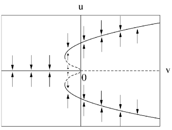
Figure 3: Solutions of equations (11) for $J^{(3)}(x_{m})<0$. Full lines show the stable solutions while dashed lines show the unstable ones. Arrows indicate the spontaneous direction of motion of a perturbation $\delta u$. This is typical of a sub-critical bifurcation.

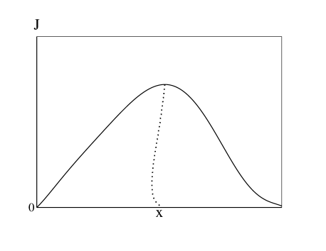
Figure 4: Typical shape of $J$ leading to a sub-critical bifurcation (with $J^{(3)}(x_{m})<0$). The dashed line corresponds to the location of the middle of horizontal secant.

For $v=0$, that is $x_{l}+x_{r}=2x_{m}=x_{tot}$, the dynamics equation writes:

$$\frac{du}{dt}=-\frac{u^{3}}{12}J^{(3)}(x_{m})-\frac{u^{5}}{960}J^{(5)}(x_{m})+...$$ (16)

The dynamics is controlled by $J^{(3)}(x_{m})$ and $J^{(5)}(x_{m})$. Return to equilibrium is no more an exponential decrease but a power law. The steady solutions of equation (16) writes at first order:

$$u = 0,$$ (17)

$$u_{\pm} = \pm\left[-80J^{(3)}(x_{m})\left(J^{(5)}(x_{m})\right)^{-1}\right]^{1/2}$$

$$\mbox{ if, }\ J^{(3)}(x_{m})J^{(5)}(x_{m})<0.$$

Their stability depends on the third and fifth derivative of $J$ at $x_{m}$. Finally, the comparison of Figures 2 and 4 shows that the symmetry of $J$ plays an important role on the bifurcation behaviour.

III.1.3 Symmetric flux function: $J(x_{m}-x)=J(x_{m}+x)$

A special attention has then to be paid to the case of a symmetric $J$, i.e. with two symmetric wings, which implies $J^{(k)}(x_{m})=0$ for all odd $k$. The dynamics equation writes at fourth order in such a case:

$$\frac{du}{dt} = -uv\left(J^{(2)}(x_{m})+\frac{v^{2}}{24}J^{(4)}(x_{m})\right)$$ (19)

$$-u^{3}\frac{v}{24}J^{(4)}(x_{m})+...$$

Where $J^{(2)}(x_{m})<0$.
Let us first neglect the higher order terms $J^{(4)}(x_{m})$ …, and consider the problem near $v=0$. As $J^{(2)}(x_{m})<0$, the solution $u=0$ is stable for $v<0$ and unstable for $v>0$.

So, at $v=0$, there is a continuous set of equilibrium states, since $\frac{du}{dt}=0$ whatever $u$. So, all initial states are equilibrium states: keeping $v=0$, and starting from any definite state $u=u_{0}$, $u_{0}$ is a steady state. Suppose now that the system passes spontaneously to $u_{1}$ due to some perturbation, in this case the new $u_{1}$ state also is the new steady state and the system will be fully driven by perturbation or uncontrolled noise that generates transition from $u_{0}$ to $u_{1}$.

As we will see, such a bifurcation trend is important because it leads to generate extremely large fluctuation, larger than a critical bifurcation. We can then call this bifurcation an hypercritical bifurcation. Its diagram is displayed on Figure 5. Figure 6 shows typical functions $J$ which give rise to a hypercritical bifurcation, with the vertical dotted line representing the location of the middles of horizontal secant.

This bifurcation is particularly interesting from an experimental point of view because its dynamics is completely driven by the existing noise, and because any extensive quantity is subject to noise due to the discreetness of nature at some microscopic finite scale. Indeed, no matter some mechanism exists to absorb any perturbation or to make the perturbation grow, the system is then entirely driven by the noise when it is at this working point even if it covers only equilibrium states.

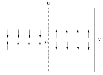
Figure 5: Solutions of equations (11) for $v=0$ and $du/dt=0$ for all $u$. Full line shows the stable solution while dashed line shows the unstable ones. The dot-dashed line shows the set of solutions which are neither stable nor unstable. Arrows indicate the spontaneous direction of motion of a perturbation $\delta u$. Hypercritical bifurcation.

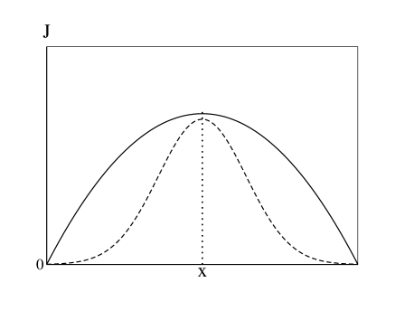
Figure 6: Two examples of the shape of $J$ corresponding to a hypercritical bifurcation when $v=0$. The curves are symmetric with respect to the maximum of $J$, $J(x_{m})$. The dashed line is the location of the middle of horizontal secant.

Does it means that the dynamics of the system at $v=0$ is a simple diffusion on the $u$ axis? Not completely, because the fluctuations that generate the motion in the $u$ direction may have specific characteristics that make the system more complex. For instance, even in the case of a random process imposed by discrete nature of the flux, as the noise is often linked to the square root of the magnitude of the flux, one shall expect already that the diffusion coefficient shall depend on the value of $u$, because the value of $J$ depends on $u$ (see Figure 6).

Since $J(0)=0$, $J(2x_{m})=0$ and the flux becomes negative when $v>0$. This is why figure 5 does not exhibit solution for $v>0$. However such solutions may appear in this hyper-critical bifurcation if some dissymmetry of $J$ is introduced at large $v$ only, i.e. above $x=2x_{m}-a$ with $a$ being small compared to $x_{m}$, so that one will find a solution for $v>0$. This requires of course that $J(x)$ remains positive for all $x>2x_{m}-a$ and tends to $0$ as $x$ tends to infinity.

III.1.4 Slightly dissymmetric flux function

If the flux function is slightly dissymmetric in the range $[0;2x_{m}]$, that is, if some of the odd derivatives at $x=x_{m}$ are not null beyond order $2k+1>5$, the bifurcation is not hypercritical stricto sensu. It means that a solution may be given. However this would require a large/infinite precision especially in the vicinity of $v=0$ to maintain its state at the predicted value. On the contrary, let us assume some existing intrinsic fluctuations. It means that the system may explore different states with time, and the wider the range explored the nearer from the symmetry the $J$ function. This is because the dissymmetry of the $J$ curve is linked to the derivatives of small order $(2k+1)$ at the maximum. So, one may expect that in the vicinity of $v=0$, the larger the order $k$ for which $J^{(2k+1)}(x_{m})$ is non null, and/or the smaller the $J^{(2k+1)}(x_{m})$ the wider the range of $u$ over which the system may spread due to fluctuations. It is then quite important to include the effect of fluctuations in the dynamics to treat correctly the problem. This will be done in the next sub-section.

III.2 Effect of the noise

The previous section was devoted to the bifurcation analysis when symmetry breaks. Expected behaviour has been described without taking into account any noise and it has been found that the kind of bifurcation depends strongly on some detail of the shape of the flux function. This makes the solution sensitive to tiny details. On the other hand, it is experimentally impossible to completely cancel the noise. So, one has then to introduce it to describe properly the physics in the vicinity of the bifurcation.
Among the questions to answer, one would like to know if the system is able to jump spontaneously from a stable solution to an other one just because of the existing noise.

This depends probably on the distance between the stable solutions and on the intensity of the noise. One can also ask how the system explores the space of stable configurations in the case of a continuous set of stable states, or how far from a stable state the system can be when it is driven by a noise of given amplitude. These questions can be addressed thanks to the computation of the fluctuation of $x$ around a stable solution. But this requires also to model the action of the noise.

Let us start with the last problem and consider a stable state $(x_{l};x_{r})$ and some perturbation $\delta x$ , i.e. $(x_{l}+\delta x,x_{r}-\delta x)$. Without perturbation, its dynamics writes:

$$\frac{dx_{l}}{dt}=J(x_{r})-J(x_{l})=0.$$ (20)

Let us slightly perturb this equation and use a Taylor expansion at first order:

$$\frac{d(x_{l}+\delta x)}{dt} = J(x_{r}-\delta x)-J(x_{l}+\delta x),$$ (21)

$$\Leftrightarrow\frac{d\delta x}{dt} \approx -\delta x\left(J^{(1)}(x_{l})+J^{(1)}(x_{r})\right),$$

$$\Leftrightarrow\frac{d\delta x}{dt} \approx -\alpha\delta x.$$ (22)

where we have used $\alpha=J^{(1)}(x_{l})+J^{(1)}(x_{r})>0$ (because it is a stable state) and $J(x_{l})=J(x_{r})$.

Let us submit this system to some random white noise of amplitude $\varepsilon(t)$, of zero mean and of variance $\sigma_{\varepsilon}^{2}$, the system obeys to a Langevin-like equation reif65 :

$$\frac{d\delta x}{dt} \approx -\alpha\delta x+\varepsilon(t).$$ (23)

A characteristic time is the time $\tau_{c}$ for the system to exchange a “particle” (or quantum) of the extensive quantity $x$: $\tau_{c}=\frac{1}{J(x_{l})+J(x_{r})}$. Assuming that $t$ is always much larger than the time for $x_{l}$ and $x_{r}$ to exchange one particle, $t\gg\tau_{c}=\frac{1}{J(x_{l})+J(x_{r})}$, equation (23) can be solved following the classic procedure as in the case of a Langevin equation and find the variance $\sigma_{\delta x}^{2}$ of $\delta x$, as a function of the variance of the noise, $\sigma_{\varepsilon}^{2}$ reif65 . We start from the general form of the solution of equation (23):

$$\delta x(t)=\delta x(0)e^{-\alpha t}+\int_{0}^{t}e^{-\alpha(t-t^{\prime})}\varepsilon(t^{\prime})dt^{\prime}.$$ (24)

As the noise $\varepsilon$ is a zero-mean random variable, $\langle\varepsilon(t)\rangle=0$, the expectation of $\delta x$ writes:

$$\langle\delta x(t)\rangle=\delta x(0)e^{-\alpha t}.$$ (25)

So, the perturbation damps, in average, from any (small) initial value with a typical time $\tau$:

$$\tau=\frac{1}{\alpha}.$$ (26)

Considering now the variance of $\delta x$ around a stable position, it is defined as:

$$\sigma_{\delta x}^{2}=\langle\delta x(t)^{2}\rangle-\langle\delta x(t)\rangle^{2}.$$ (27)

Using the square of equation (24), one obtains:

$$\sigma_{\delta x}^{2}=\int_{0}^{t^{\prime}}dt^{\prime}\int_{0}^{t}\langle\varepsilon(t^{\prime})\varepsilon(t^{\prime\prime})\rangle e^{-\alpha(t-t^{\prime})}e^{-(t^{\prime}-t^{\prime\prime})}dt^{\prime\prime}.$$ (28)

As $\varepsilon$ is a white noise, one finds:

$$\sigma_{\delta x}^{2}=\frac{\sigma_{\varepsilon}^{2}}{2\alpha}(1-\exp{(-2\alpha t)}).$$ (29)

So, when $t=0$, the variance is null because $\delta x(0)$ is known exactly. As $t$ increases from $0$, $\sigma_{\delta x}$ starts to grow as the square root of time under the effect of the noise. At larger time, the standart deviation saturates and reaches $\sigma_{\varepsilon}/\sqrt{2\alpha}$.

Note that, we shall only consider the case where $\sigma_{\delta x}$ is small since $\alpha=cste$ requires essentially $\delta x$ to be small.

So, one obtains:

$$\sigma_{\delta x}^{2}=\sigma_{\varepsilon}^{2}t,$$ (30)

if $\tau_{c}\ll t\ll\alpha^{-1}$. The width of the distribution of $\delta x$ then spreads like $\sqrt{t}$ as in a diffusion process until $t\approx\alpha^{-1}$. As $t\gg\alpha^{-1}$, the width of the distribution of $\delta x$ around a stable position is

$$\sigma_{\delta x}=\frac{\sigma_{\varepsilon}}{\sqrt{2\alpha}}.$$ (31)

III.2.1 In the vicinity of the bifurcation

Let us assume that the stable state of equilibrium is in the vicinity of $x_{m}$. If $x_{l}$ and $x_{r}$ are close to $x_{m}$ such that $J$ is almost constant, then $J(x_{l})\approx J(x_{r})$ and $\alpha\approx cste\ll 1$, one obtains (when $t\ll\alpha^{-1}$):

$$\sigma_{\delta x}^{2}\approx\sigma_{\varepsilon}^{2}t.$$ (32)

$\delta x$ undergoes a diffusion process and nothing prevents from the spreading of the perturbation as long as $\delta x$ is small enough, that is, as long as $\sigma_{\delta x}$ is smaller than the size of the region where $\alpha\ll 1$. In this case, the diffusion coefficient writes $D=\sigma_{\varepsilon}^{2}/2$. The time needed by the perturbation to reach any small distance $d$ from an initial position is:

$$t_{d}\approx\frac{d^{2}}{D}=\frac{2d^{2}}{\sigma_{\varepsilon}^{2}}.$$ (33)

So, if two stable states are close enough, the sytem will pass from one stable state to the other with a frequency equal to $\sigma_{\varepsilon}^{2}/2d^{2}$. diffusion has then two effetct: the broadening of each steady state and the jump from one steady state to the other.

In the case of a supercritical bifurcation, we may try to define when the two ”steady” states remain separated and detectable as such. It occurs when the standard-deviation (due to noise) of a single steady state (without noise) is smaller than the distance between the two steady states $x_{l}=x_{r}=x_{tot}/2$ and $x_{m}$. As the standard deviation $\sigma_{\delta x}$ is given by equation 31, it imposes:

$$\sigma_{\delta x}^{2}=\frac{\sigma_{\varepsilon}^{2}}{2\alpha}<(x_{m}-x_{l})^{2}.$$ (34)

With $x_{m}-x_{l}=-v/2$ and $\alpha=2J^{(1)}(x_{l/r})\approx\frac{1}{2}vJ^{(2)}(x_{m})$, one obtains:

$$\frac{\sigma_{\varepsilon}^{2}}{2vJ^{(2)}(x_{m})} < \frac{v^{2}}{4},$$ (35)

$$\Rightarrow\sigma_{\varepsilon}^{2} < \frac{1}{2}v^{3}J^{(2)}(x_{m}).$$ (36)

If this inequality is not satisfied, the two branches of stable solutions in figure 2 can not be observed and the bifurcation is not detected as long as $v$ is too small.

In the same way, when a subcritical bifurcation occurs, as displayed in figure 4, the jump from the single stable solution $u=0$ to one of the two others may occur before the maximum of the flux function, i.e. before $v=0$, so that for strong enough noise or little subcriticality, the bifurcation may look as a supercritical one.

Finally, if one considers a hypercritical bifurcation, the flux function is symmetric with respect to its maximum, $\alpha$ is always null and $J(x_{l})=J(x_{r})$. All the states are equilibrium ones and, because of the noise, $x_{l}$ and $x_{r}$ constantly fluctuates between all of them. As a conclusion the nature the noise can hide the true nature of the bifurcation.

III.2.2 Far from the bifurcation

On the other hand, if the stable state of equilibrium corresponds to different $x_{l}$ and $x_{r}$ such that $\alpha\approx cste\gg 1$, the variance $\sigma_{\delta x}^{2}$ tends to a finite value:

$$\sigma_{\delta x}^{2}\approx\sigma_{\varepsilon}^{2}/2\alpha.$$ (37)

It means that the spreading of $\delta x$ due to the noise is balanced by the damping due to $\alpha$. Assuming that $\alpha$ is constant, $\delta x$ is a Gaussian random variable having the following probability density function:

$$f_{\delta x}(X) = \frac{1}{\sigma_{\delta x}\sqrt{2\pi}}e^{-\frac{X^{2}}{2\sigma_{\delta x}^{2}}},$$ (38)

$$= \sqrt{\frac{\alpha}{\pi\sigma_{\varepsilon}^{2}}}e^{-\frac{\alpha X^{2}}{\sigma_{\varepsilon}^{2}}}.$$ (39)

The probability to jump from a stable solution to another one is the probability to have $\delta x$ larger than the distance $d$ from the initial stable state to the frontier of its basin of attraction. As $\alpha$ has a damping effect, one expects that the probability for a jump to occur should decrease as $\alpha$ increases. From equation (39), one can write this probability:

$$P(\delta x>d)=\frac{1}{2}\left[1-\mbox{erf}\left(\frac{\sqrt{2}\alpha d}{\sigma_{\varepsilon}}\right)\right],$$ (40)

where $\mbox{erf}(.)$ denotes the error function and $P(\delta x>d)$ decreases as $\alpha$ increases as expected.

In fact, the latter result can be applied if a supercritical or a subcritical bifurcation has occured and not after a hypercritical bifurcation. After a hypercritical bifurcation the only result one can write is that the life expectancy, $t_{l}$, of a stable state is proportional to the time needed by the noise to make the two boxes exchange one particle:

$$t_{l} \propto \frac{1}{\sigma_{\varepsilon}^{2}},$$ (41)

$$\propto \frac{1}{J(x_{l})+J(x_{r})}.$$ (42)

So, as $J(x_{l})+J(x_{r})$ tends to zero, the corresponding equilibrium state will be observed during a time much longer than the one for which $J(x_{l})+J(x_{r})$ is large. Thus, from an experimental point of view, much attention has to be paid to the interpretation of the experimental results. Indeed, a state may be wrongly interpreted as a non equilibrium one if $J(x_{l})+J(x_{r})$ is large.

IV Experimental part

A well-known experiment involving a system of two communicating containers partially filled with macroscopic spherical particles is the so-called granular “Maxwell demon”. When such compartments are shaken together at same frequency and amplitude, it has been often quoted that, under some circumstances, one compartment empties spontaneously in the other schlichting96 . This symmetry breaking comes from the fact that the outgoing flux function is not monotonic as the number of particles increases: it first grows as the number of beads $N$ increases and, as $N>N_{max}$, decreases because the dissipation becomes more important. Then, it seems to be a relevant experiment to test the prediction of the previous section. Note that this experiment has been studied in eggers99 . He used the equality of the outgoing flux from each box as the equilibrium condition, and a continuous model taking into account that the effective granular temperature decreases when the density of particles increases. He concludes that the symmetry breaking follows a second order phase transition. However, it has been pointed out that the Egger’s approach suffers some discrepancies with respect to experiments pierre02 and that a thermodynamics analogy to describe such a system is questionable pierre02bis . An other approach has been proposed brey01 when the size of the hole connecting both compartments is larger than the mean free path of the particles. It is based on the pressure balance between the two boxes and leads to the conclusion that beyond a critical value of the number of particles, the symmetry breaks spontaneously. Anyway, this surprising behaviour has motivated many experiments using mixtures of different particles, different boundaries conditions or different number of compartments for instance lipowski02 ; barrat03_2 ; mikkelsen05 ; vandermeer06 . But the influence of the experimental parameters on the shape of the flux function, and then on the kind of bifurcation leading to the symmetry breaking, has not yet been addressed.

In the present experiment, we study a granular Maxwell demon experiment using the outgoing flux function $J$ to forecast what kind of transition occurs when the symmetry breaks. The control parameter is the number of particles $N$ and the analysis is made for three different frequencies. We use a single vibrated box to measure $J$ as a function of the number of particles $N$ that it contains and of the frequency of excitation. Our analysis is based on the same equilibrium condition than the one used in eggers99 , that is on the balance of the outgoing flux between the two compartments. Note that because the number of balls is discrete, there is an intrinsic noise in our experiments but we will see that it is nevertheless possible to identify different bifurcations. It is also important to note that in the case of two vibrating boxes and if $N$ is large enough, interactions between particles coming from one compartment to the other could occur in the vicinity of the route between the boxes. However, this latter would occur at much larger densities. It would lead in this case to a flux function depending on the number of particles in both boxes which is not our purpose here.

IV.1 Experimental apparatus

The experimental apparatus is shown on Figure 7. A single box of dimension $L=20mm$, $H=30mm$, $l=12mm$, with a narrow slit on one side at height $10mm$ and of width $3mm$, is partially filled with $N\approx 680$ steel spheres of diameter $1mm$.

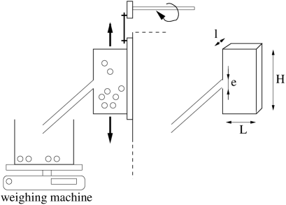
Figure 7: Experimental apparatus.

The box is fixed on a sliding girder connected to a crankshaft and a rotating wheel. It allows to impose a linear oscillation to the box, $A\sin{(2\pi ft)}$ where $f$ and $A$ are the frequency and the amplitude of the sinusoidal oscillation respectively: $f\in[26Hz-43Hz]$ and $A=1.25\ mm$. The mechanical device is mounted on a massive steel socle in order to avoid any perturbation.

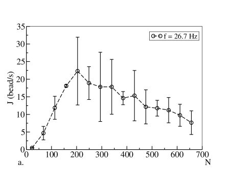
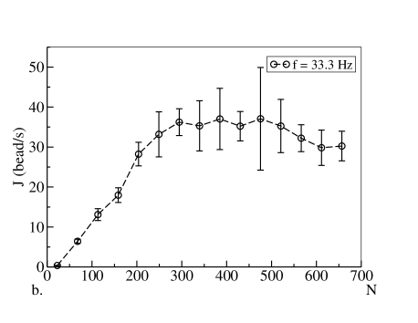
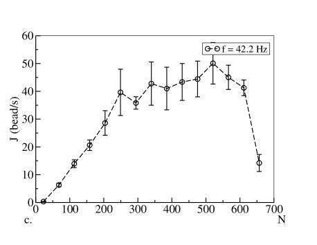
Figure 8: Experimental flux as a function of the number of particles in the container shaked at frequency $f$. a. $f=26.7Hz$, b. $f=33.3Hz$, c. $f=42.2Hz$.

The frequency is imposed with an electrical motor and controlled, during each experiment, thanks to a tachometer to measure the fluctuaction of the frequency. The maximum amplitude of these fluctuations is smaller than $2\%$ of the imposed frequency. When beads leave the vibrating compartment, a long tube bring them to a repository with a soft bottom such that grains do not bounce. The evolution of the mass of the content’s repository is measured each $0.5s$ thanks to a weighing machine with a precision much less than $10^{-3}g$ (which is the tool accuracy), because of parasite effect that includes mechanical vibration and ball collision with bottom. Data are then recorded with LabVIEW Software on a computer and smoothened. For a given frequency $f$, the outgoing flux $J(t)$ is derived from the temporal mass evolution. This allows to finally plot $J$ as a function of the number of beads, $N$, remaining in the vibrating box.

IV.2 Experimental results

Figure 8 shows the outgoing flux, $J(N)$, obtained for three imposed frequencies $f=26.7Hz$, $33.3Hz$ and $42.2Hz$. Each plotted curve is the mean of several experiments. They all starts from $J(0)=0$, increases until it reaches a maximum and then starts to decrease. This behaviour reminds us of the different shapes of flux function we studied in the previous section.

One can already note that Figure 8.a has a left wing steeper than the right wing and that 8.b displays a right wing steeper than the left one. So, if the experiments are described correctly by the model of the previous section and even with some noise, we may be tempted to conclude that the kind of bifurcation changes as the frequency of vibration increases.

Assuming a Gaussian white noise, the standard deviation (s.d.) is computed by multiplying the empirical s.d. with the $5\%$-quantile of the Student law with $p$ degrees of liberty, where $p$ is the number of experiments bouquin_stat . Indeed, it is a classical way to proceed when the number of experiments is small. As one can expect, at fixed frequency, the uncertainty is large when the flux is large. Note that three experiments have been made for $f=26.7Hz$ and nine experiments have been achieved for $f=33.3Hz$ and $f=42.2Hz$. This explains why the uncertainties seem larger for $f=26.7Hz$ than for the two other frequencies used.

One has also to mention that in these experiments and for the largest values of $N$, the number $n$ of layers of particles is $n\approx 3$. The distance between the top layer and the slit is then $D\approx 7\ mm$. For the highest frequency, $f=42.2\ Hz$, the height reached by a particle initially at rest is $h\approx 5.6\ mm$. As $h\approx D$, the density of particles in the vicinity of the slit might be sufficiently large such that interactions occur between the beads of the two boxes. It means that the tail of each curve in Figure 8, that is for the largest number of particles, could have been modified by the high concentration of particles near the slit. In this case, this would involve another equilibrium condition than the one on flux and then an approach using fluid parameter, similar to brey01 for instance, could be more suitable to this problem.

Anyway, if one assumes that interactions do not occur, one can use the result of section III. Each curve is then fitted to a polynomial function of degree chosen thanks to a likelihood ratio test bouquin_stat . One then computes the value $N_{m}$ for which $dJ/dN=0$ and the successive derivatives of $J$ at $N_{m}$. The result is that Figures 8.a, 8.b and 8.c correspond to supercritical, hypercritical and subcritical bifurcations respectively as $N$ increases. As forecast previously, the kind of bifurcation depends on the frequency used during an experiment.
Let us discuss briefly how the system converge to an equilibrium stable state and the effect of the noise. The convergence to a stable state depends on the sum of the derivatives of the flux function at $N_{l}$ and $N_{r}$. However, as $N$ is a discrete value, the flux of $N$ is discrete and fluctuates, and the exact equilibrium state is not reachable. It results a standard deviation at $N_{l}$ and $N_{r}$ which is inversely proportional to the sum of both slopes around $N_{l}$ and $N_{r}$ (see equation 31).

Recently, Mikkelsen et al mikkelsen05 studied a granular Maxwell demon experiment and the effect of statistical fluctuation on critical phenomena. Their numerical simulations show qualitatively the same kind of flux curves as ours, as the frequency increases. The symmetry breaking is studied with the frequency as the control parameter and with different total number of particles $N$ to highlight the effect of a noise. They find that, at fixed $N$, the transition is supercritical when the frequency becomes larger than a critical threshold. However, according to our analysis, it can be either supercritical, subcritical or hypercritical when $N$ becomes larger than a threshold, the type of bifurcation depending on the frequency of vibration. They also find that they are faced with a supercritical bifurcation when the flux curve is symmetric whereas our study proves that the bifurcation is hypercritical and that the system is driven by the noise in this case. This shows how the type of bifurcation depends on the control parameter used.
As a final remark, it is worth mentionning that a Maxwell demon experiment checks directly the breaking of symmetry. It tests then the shape of the flux function near its maximum and cannot then be considered as a proof of any modelling of the flux function far from this maximum. Consequently, most of the flux function assumed in the litterature cannot be considered as settled on experimental evidence.

V Conclusion

In conclusion, we have proposed a theoretical analysis of the behaviour of two subsystems able to exchange each other some part of their internal quantity thanks to a flux function $J$. We have shown that when $J$ is not monotonic, a bifurcation can occur leading to different equilibrium states. The type of bifurcation is then found to depend on the detail of the shape of the flux function near its maximum. In particular, we have pointed out a new kind of bifurcation called hypercritical when the shape of the flux function is symmetric with respect to its maximum. In this case, a continuum of solution exists making the dynamics of the system govern by the noise. In the other cases, the noise, if large enough, is found to have an impact on the conclusion concerning the kind of bifurcation which appears. In the last part of this paper, we have presented a simple granular Maxwell demon experiment to investigate the kind of transition occurring when the symmetry breaks. Unlike previous experiments, we use the number of particles as the control parameter with different frequencies of vibration $f$. Our results show that different bifurcation, including the hypercritical one, occur depending on $f$. This behaviour was not pointed out before neither experimentally, nor numerically, not theoretically. It could then allow to investigate new kind of bifurcation.
However the detection of the true nature of bifurcation (supercritical vs. subcritical, etc) is made difficult due to the little number of grains (and by the noise it induces) in the case of a Maxwell demon experiment. This is easier if one uses directly the flux function which gives directly the symmetry of the curve. In turn this means the use of a single half box. We believe that a Maxwell demon experiment with $100$ balls only test the presence of a bifurcation, but not the precise shape of the flux function near its maximum or further in the tails. So, previous Maxwell demon experiments can not be considered as a test of the validity of any modelling of the flux function far from this maximum as it is sometimes done in the literature.

Acknowledgements:

Centre National d’Etudes Spatiales (CNES) is gratefully thanked for financial support.

References

- (1) P. G. Drazin and W. H. Reid, “Hydrodynamic stability”, Cambridge University Press, Ed. Cambridge, ISBN 0-521-28980-7 (1997).
- (2) J. D. Murray, “Mathematical biology, I: An Introduction (Third Edition)”, Interdisciplinary applied mathematics, Ed. Springer, ISBN 0-387-95223-3 (2002).
- (3) Z. Mei, “Numerical bifurcation analysis for reaction-diffusion equations”, Springer Series in Computational Mathematics, Ed. Springer, ISBN 3-540-67296-6 (2000).
- (4) J. D. Crawford, “Introduction to bifurcation theory”, Rev. Mod. Phys. 63, p. 991 (1991).
- (5) P. Berge, Y. Pomeau, Ch. Vidal, “L’ordre dans le chaos. Vers une approche deterministe de la turbulence” (in french), Enseignement des sciences, Ed. Hermann (Paris), ISBN 2705659803 (1984).
- (6) P. Manneville, “Dissipative structures and weak turbulence”, Perspectives in physics, Ed. Academic Press, ISBN 0-12-469260-5 (1990).
- (7) H. J. Schlichting and V. Nordmeier, “Strukturen im Sand” (in german), Math. Naturwiss. Unterr. 49, p. 323 (1996).
- (8) J. Eggers, “Sand as Maxwell’s Demon”, Phys. Rev. Lett. 83 (25), p. 5322 (1999).
- (9) Langevin P., “Sur la théorie du mouvement brownien” (in french), Comptes Rendus 146, p. 530 (1908). F. Reif, “Fundamentals of statistical and thermal physics”, Ed. McGraw-Hill, New York (1965).
- (10) P. Jean, H. Bellenger, P. Burban, L. Ponson and P. Evesque, “Phase transition or Mawxwell’s demon in granular gas?”, Poudres et Grains 13 (3), p. 27 (2002).
- (11) P. Evesque, “Are temperature and other thermodynamics variables efficient concept for describing granular gases and/or flows?”, Poudres et Grains 13 (2), p. 20 (2002).
- (12) J. Javier Brey, F. Moreno, R. García-Rojo and M. J. Ruiz-Montero, “Hydrodynamic Maxwell Demon in granular systems”, Phys. Rev. E 65, p. 11305 (2001).
- (13) A. Lipowski and M. Droz, “Urn model of separation of sand”, Phys. Rev. E 65, p. 31305 (2002).
- (14) A. Barrat and E. Trizac, “A molecular dynamics ’Maxwell Demon’ experiment for granular mixtures”, Molecular Phys. 101 (11), p. 1713 (2003).
- (15) R. Mikkelsen, K. van der Weele, D. van der Meer, M. van Hecke and D. Lohse, “Small-number statistics near the clustering transition in a compartmentalized granular gas”, Phys. Rev. E 71, p. 41302 (2005).
- (16) D. van der Meer, K. van der Weele and P. Reimann, “Granular fountains: Convection cascade in a compartmentalized granular gas”, Phys. Rev. E 73, p. 61304 (2006).
- (17) Bickel P. J. and Doksum K. A. “Mathematical statistics: Basic ideas and selected topics” Holden-day series in probability and statistics, Ed. Holden-Day, ISBN 0-8162-0784-4 (1977).